
The Study of Various Regression Models Establishment to Identify Farmland Soil Moisture Content at Different Depths Using Unmanned Aerial Vehicle Multispectral Data: A Case in North China Plain
 ,
,
Abstract
:1. Introduction
2. Materials and Methods
2.1. Field Experiment
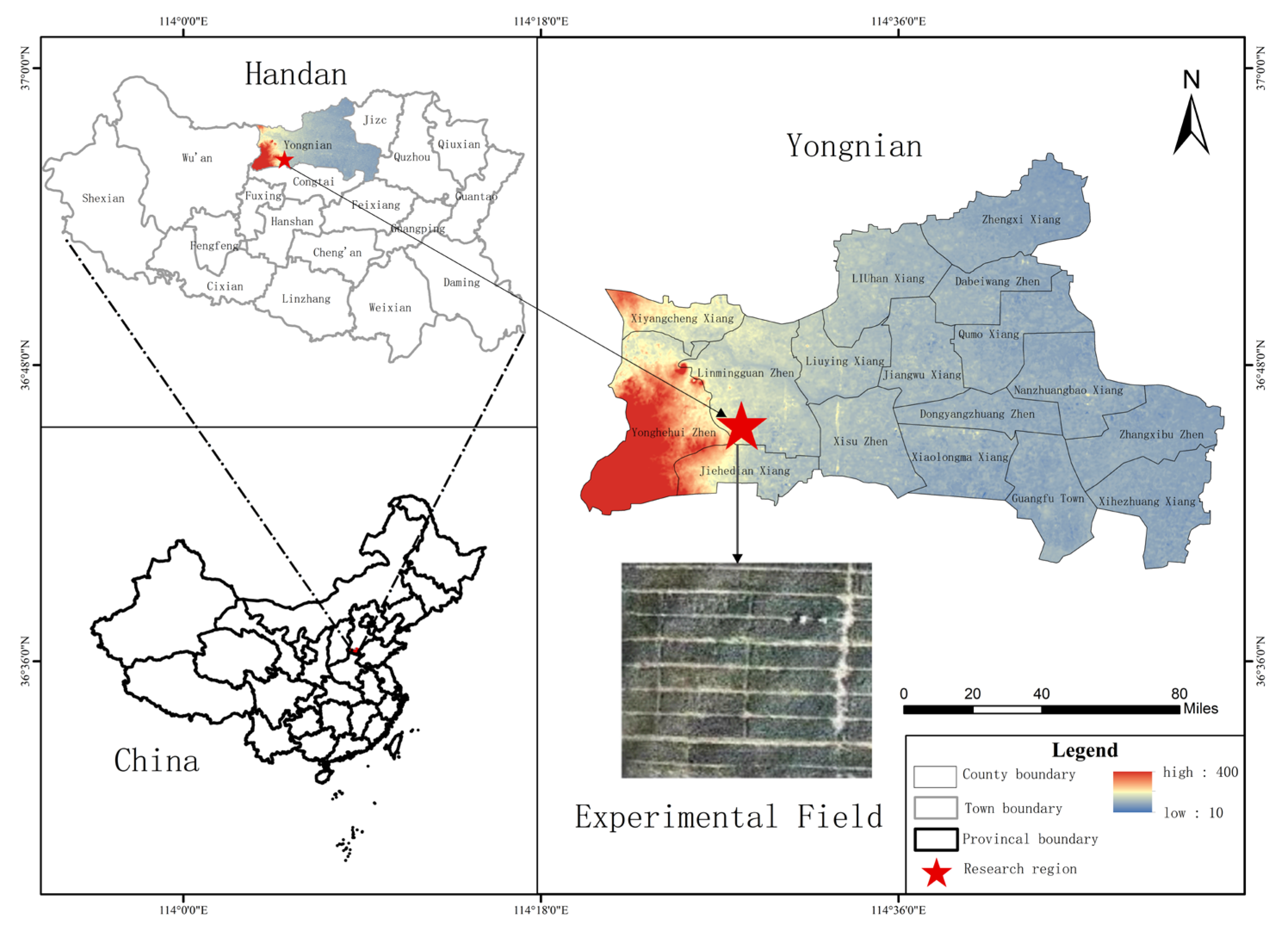
2.1.1. Experimental Area
2.1.2. Experimental Arrangement
2.1.3. Remote Sensing Data Acquisition
2.1.4. Ground Data Acquisition
2.1.5. Data Processing
2.2. Regression Models
2.2.1. Unary Linear Regression (ULR)
2.2.2. Multivariate Linear Regression (MLR)
2.2.3. Ridge Regression (RR)
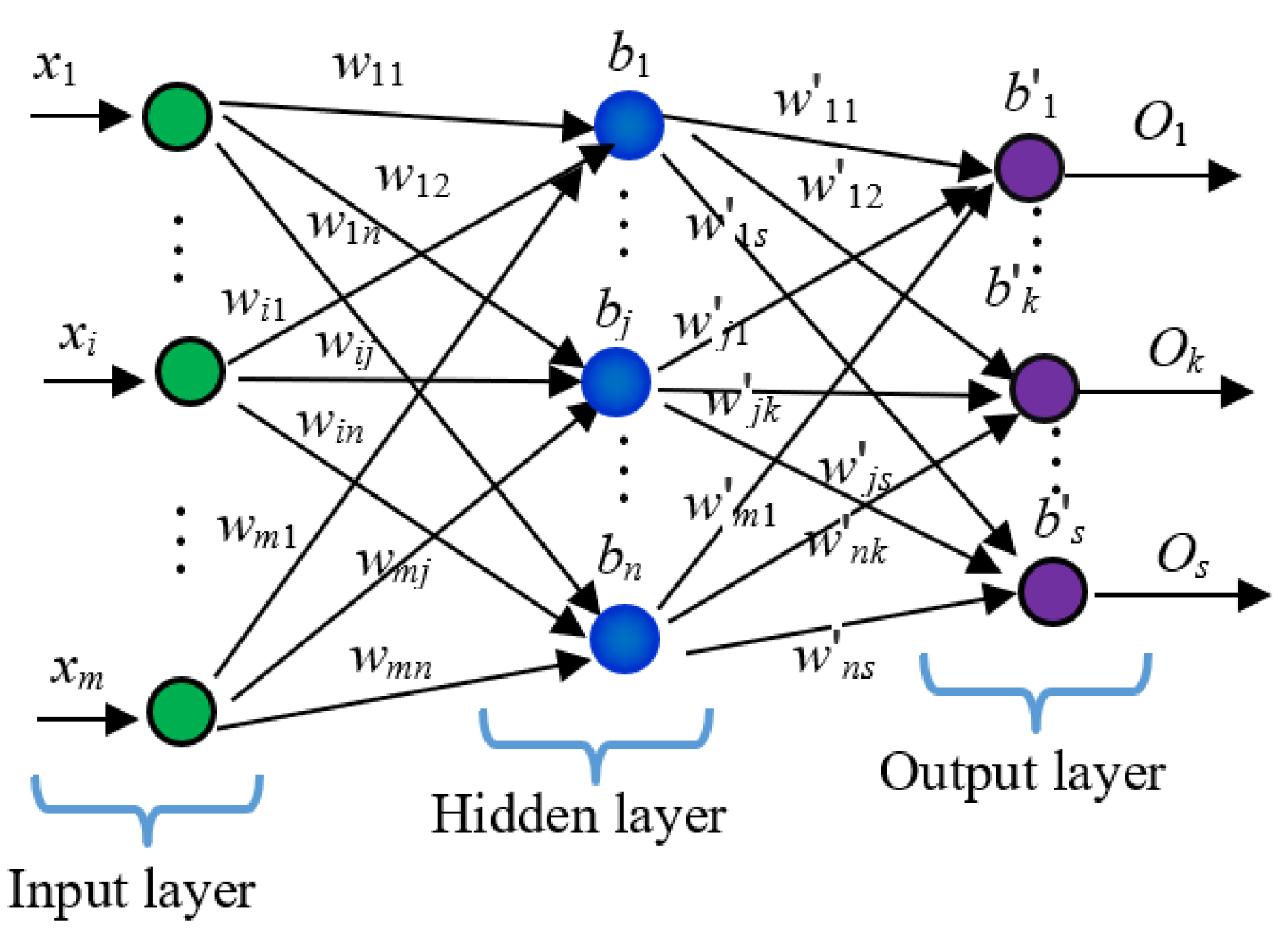
2.2.4. BP Neural Network
3. Results and Discussion
3.1. Field Experiment Unary Linear Regression (ULR)
3.2. Multivariate Linear Regression (MLR)
3.3. Ridge Regression (RR)
3.4. BP Neural Network
4. Conclusions
Author Contributions
Funding
Data Availability Statement
Acknowledgments
Conflicts of Interest
References
- Döpper, V.; Rocha, A.D.; Berger, K.; Gränzig, T.; Verrelst, J.; Kleinschmit, B.; Förster, M. Estimating soil moisture content under grassland with hyperspectral data using radiative transfer modelling and machine learning. Int. J. Appl. Earth Obs. Geoinf. 2022, 110, 102817. [Google Scholar] [CrossRef] [PubMed]
- Singh, H.V.; Thompson, A.M. Effect of antecedent soil moisture content on soil critical shear stress in agricultural watersheds. Geoderma 2016, 262, 165–173. [Google Scholar] [CrossRef]
- Al-Karaghouli, A. Influence of soil moisture content on soil solarization efficiency. Renew. Energy 2001, 24, 131–144. [Google Scholar] [CrossRef]
- Gupta, A.; Rico-Medina, A.; Caño-Delgado, A.I. The physiology of plant responses to drought. Science 2020, 368, 266–269. [Google Scholar] [CrossRef] [PubMed]
- Limin, P.; Yingyi, C.; Yan, X.; Jun, L.; Huazhong, L. A model for soil moisture content prediction based on the change in ultrasonic velocity and bulk density of tillage soil under alternating drying and wetting conditions. Measurement 2021, 189, 110504. [Google Scholar] [CrossRef]
- Tian, J.; Yue, J.; Philpot, W.D.; Dong, X.; Tian, Q. Soil moisture content estimate with drying process segmentation using shortwave infrared bands. Remote Sens. Environ. 2021, 263, 112552. [Google Scholar] [CrossRef]
- Guo, J.; Bai, Q.; Guo, W.; Bu, Z.; Zhang, W. Soil moisture content estimation in winter wheat planting area for multi-source sensing data using CNNR. Comput. Electron. Agric. 2022, 193, 106670. [Google Scholar] [CrossRef]
- Wigmore, O.; Mark, B.; McKenzie, J.; Baraer, M.; Lautz, L. Sub-metre mapping of surface soil moisture in proglacial valleys of the tropical Andes using a multispectral unmanned aerial vehicle. Remote Sens. Environ. 2019, 222, 104–118. [Google Scholar] [CrossRef]
- Jiao, G.; Jian, L.; Jifeng, N.; Wenting, H. Construction and Verification of soil moisture inversion model on farmland surface based on sentinel multi-source data. Trans. Chin. Soc. Agric. Eng. 2019, 35, 71–78. [Google Scholar]
- Meixia, W.; Wenlan, F.; Yangzong, Z.; Yongqian, W.; Xiaojun, N. Study on synergistic inversion of surface soil moisture in Northern Tibet based on optical and microwave remote sensing. Soil 2019, 51, 1020–1029. [Google Scholar]
- Zhang, Z.; Wang, H.; Han, W.; Bian, J.; Chen, S.; Cui, T. Inversion of soil moisture content based on multispectral remote sensing of UAVs. Trans. Chin. Soc. Agric. Mach. 2018, 49, 173–181. [Google Scholar]
- Qiyuan, W. Inversion of soil moisture in bare soil based on multi spectral remote sensing. Int. J. Min. Sci. Technol. 2020, 5, 608–615. [Google Scholar]
- Zhang, X.; Uwimpaye, F.; Yan, Z.; Shao, L.; Chen, S.; Sun, H.; Liu, X. Water productivity improvement in summer maize—A case study in the North China Plain from 1980 to 2019. Agric. Water Manag. 2021, 247, 106728. [Google Scholar] [CrossRef]
- Sekiya, N.; Yano, K. Water acquisition from rainfall and groundwater by legume crops developing deep rooting systems determined with stable hydrogen isotope compositions of xylem waters. Field Crops Res. 2002, 78, 133–139. [Google Scholar] [CrossRef]
- Xiaojing, L.; Guoqing, C.; Liang, W.; Yujie, C.; Lan, W.; Xiaoyu, L.; Xueguo, L. Study on Inversion model of soil water content of winter wheat based on SOC710VP hyperspectral imager. J. Irrig. Drain. 2019, 38, 35–42. [Google Scholar]
- Xiaoguang, Z.; Fanchang, K. Spectral model of coastal saline soil moisture based on simulated evaporation data. J. Irrig. Drain. 2020, 39, 14–19. [Google Scholar]
- Yu-le, S.; Zhong-yi, Q.; Quan-ming, L.; Li-ping, W. Dynamic Study of regional soil moisture content based on multi-source remote sensing co-inversion. J. Southwest Univ. 2020, 42, 46–53. [Google Scholar]
- Chung, J.; Lee, Y.; Kim, J.; Jung, C.; Kim, S. Soil moisture content estimation based on Sentinel-1 SAR imagery using an artificial neural network and hydrological components. Remote Sens. 2022, 14, 465. [Google Scholar] [CrossRef]
- Yin, C.S.; Liu, Q.M.; Wang, C.J.; Wang, F.Q. Inversion of soil moisture by surface spectral measurement combined with active microwave remote sensing. Southwest China J. Agric. Sci. 2022, 35, 2595–2602. [Google Scholar]
- Chu, P.; Zhang, Y.; Yu, Z.; Guo, Z.; Shi, Y. Winter wheat grain yield, water use, biomass accumulation and remobilization under tillage in the North China Plain. Field Crops Res. 2016, 193, 45–53. [Google Scholar] [CrossRef]
- Shijie, Z.; Zhihua, H. Analysis of the dynamics and genesis of groundwater level in Handan area of North China Plain. People’s Yellow River 2019, 41, 25–27, 36. [Google Scholar]
- Wang, H.; Zhang, Z.; Fu, Q.; Chen, S.; Bian, J.; Cui, T. Inversion of Soil Moisture Content Based on Multispectral Remote Sensing Data of Low Altitude UAV. Water Sav. Irrig. 2018, 90–94. [Google Scholar]
- Liu, Y.; Guo, L.; Huang, Z.; López-Vicente, M.; Wu, G. Root morphological characteristics and soil water infiltration capacity in semi-arid artificial grassland soils. Agric. Water Manag. 2020, 235, 106153. [Google Scholar] [CrossRef]
- Chen, J.; de Hoogh, K.; Gulliver, J.; Hoffmann, B.; Hertel, O.; Ketzel, M.; Bauwelinck, M.; van Donkelaar, A.; Hvidtfeldt, U.A.; Katsouyanni, K.; et al. A comparison of linear regression, regularization, and machine learning algorithms to develop Europe-wide spatial models of fine particles and nitrogen dioxide. Environ. Int. 2019, 130, 104934. [Google Scholar] [CrossRef] [PubMed]
- Yang, Y.; Sun, L.; Guo, C. Aero-material consumption prediction based on linear regression model. Procedia Comput. Sci. 2018, 131, 825–831. [Google Scholar] [CrossRef]
- Tabrizi, S.S.; Sancar, N. Prediction of Body Mass Index: A comparative study of multiple linear regression, ANN and ANFIS models. Procedia Comput. Sci. 2017, 120, 394–401. [Google Scholar] [CrossRef]
- Montgomery, D.C.; Peck, E.A.; Vining, G.G. Introduction to Linear Regression Analysis; John Wiley & Sons: Hoboken, NJ, USA, 2021. [Google Scholar]
- Liying, W.; Qingjiao, C.; Zhenxing, Z.; Seyedali, M.; Weiguo, Z. Artificial rabbits optimization: A new bio-inspired meta-heuristic algorithm for solving engineering optimization problems. Eng. Appl. Artif. Intell. 2022, 114, 105082. [Google Scholar] [CrossRef]
- Adnane, B.; Wilfred, O.; Ho-Chul, S.; Hannah, V.C.; Jane, R.; Aziz, S.; Mohamed El, G. Evaluation of pedotransfer functions to estimate some of soil hydraulic characteristics in North Africa: A case study from Morocco. Front. Environ. Sci. 2023, 11, 120. [Google Scholar] [CrossRef]
- Zhu, X.-C.; Cao, R.-X.; Shao, M.-A. Spatial simulation of soil-water content in dry and wet conditions in a hectometer-scale degraded alpine meadow. Land Degrad. Dev. 2018, 30, 278–289. [Google Scholar] [CrossRef]


| Depth (cm) | Band 1 (470 nm) | Band 2 (550 nm) | Band 3 (660 nm) | Band 4 (690 nm) | Band 5 (710 nm) | Band 6 (810 nm) |
|---|---|---|---|---|---|---|
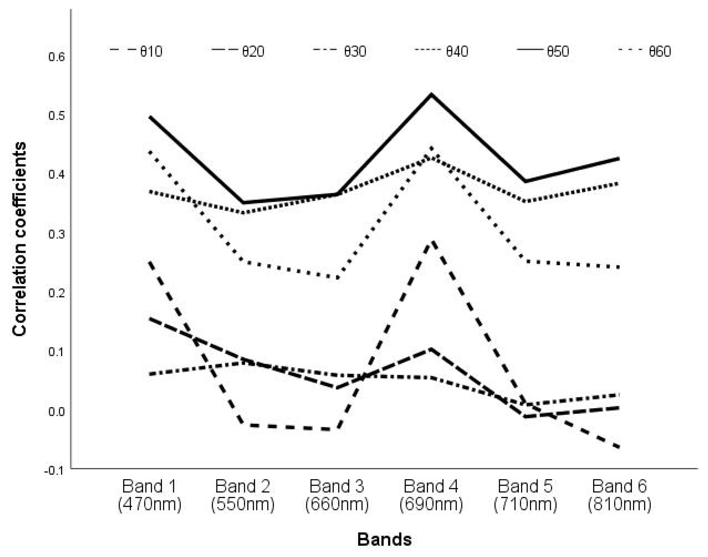
| 10 | 0.250 | −0.026 | −0.034 | 0.288 | 0.010 | −0.064 |
| 20 | 0.154 | 0.085 | 0.037 | 0.102 | −0.012 | 0.003 |
| 30 | 0.060 | 0.079 | 0.058 | 0.054 | 0.008 | 0.025 |
| 40 | 0.369 * | 0.333 | 0.364 * | 0.426 * | 0.352 * | 0.383 * |
| 50 | 0.496 ** | 0.350 * | 0.364 * | 0.533 ** | 0.386 * | 0.425 * |
| 60 | 0.437 * | 0.250 | 0.223 | 0.442 * | 0.251 | 0.241 |
| Depths | Regression Equations | RMSE | F | p |
|---|---|---|---|---|
| 60 | y = 0.222b − 13.343 | 2.864 | 7.521 | 0.010 |
| 50 | y = 0.239b − 14.257 | 2.419 | 12.327 | 0.001 |
| 40 | y = 0.164b − 4.939 | 2.216 | 6.882 | 0.013 |
| Depths | Regression Equations | RMSE | F | P |
|---|---|---|---|---|
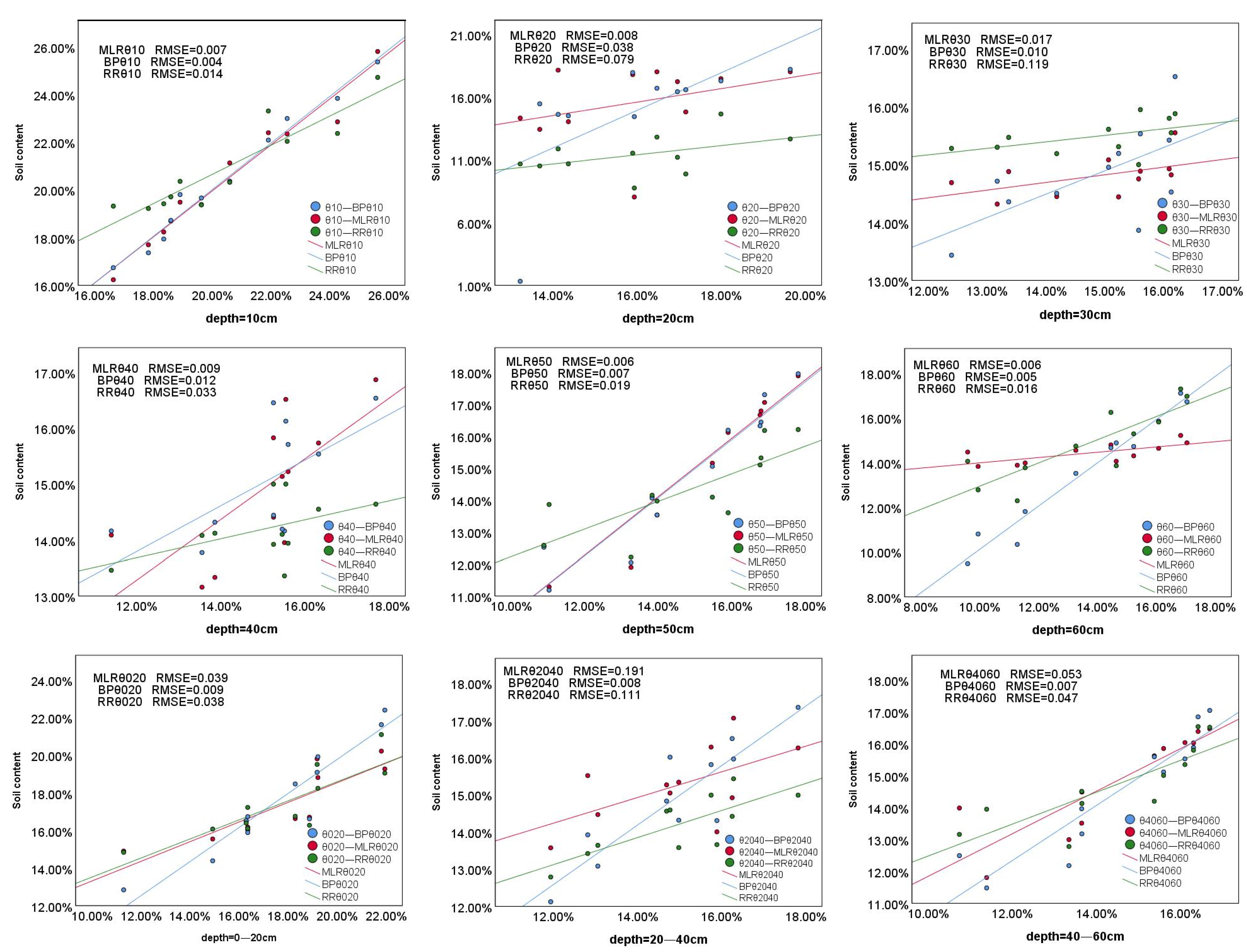
| 60 | y = 0.511b1 + 1.319b2 − 1.868b3 + 0.7904b4 − 1.022b5 + 1.131b6 + 86.511 | 0.006 | 19.756 | 0.006 |
| 50 | y = 0.596b1 + 0.262b2 − 0.619b3 + 0.613b4 − 1.170b5 + 1.032b6 + 52.157 | 0.006 | 6.615 | 0.04 |
| 40 | y = 0.237b1 − 0.481b2 + 0.555b3 + 0.314b4 − 0.739b5 + 0.314b6 + 5.667 | 0.009 | 0.460 | 0.811 |
| 30 | y = −0.313b1 + 0.998b2 − 0.895b3 + 0.337b4 − 0.437b5 + 0.436b6 + 55.811 | 0.017 | 0.450 | 0.818 |
| 20 | y = 2.147b1 − 2.624b2 + 3.416b3 + 0.296b4 − 2.604b5 − 0.111b6 − 17.376 | 0.008 | 2.148 | 0.24 |
| 10 | y = 2.375b1 − 1.744b2 + 1.095b3 + 0.006b4 − 1.192b5 + 0.168b6 + 36.507 | 0.007 | 30.036 | 0.003 |
| 0–20 | y = 2.261b1 − 2.184b2 + 2.256b3 + 0.151b4 − 1.898b5 + 0.028b6 + 9.566 | 0.039 | 6.44 | 0.046 |
| 20–40 | y = 0.69b1 − 0.702b2 + 1.025b3 + 0.316b4 − 1.260b5 + 0.213b6 + 14.701 | 0.191 | 2.643 | 0.183 |
| 40–60 | y = 0.448b1 + 0.367b2 − 0.644b3 + 0.572b4 − 0.977b5 + 0.826b6 + 48.112 | 0.053 | 4.208 | 0.093 |
| Soil Depth | Regression Equations | RMSE | p |
|---|---|---|---|
| 10 | y = 0.0075b1 − 0.0021b2 − 0.0021b3 + 0.0032b4 − 0.0031b5 − 0.0008b6 + 0.3075 | 0.014 | 0.015 |
| 20 | y = 0.0054b1 + 0.0011b2 + 0.0002b3 + 0.0022b4 − 0.0044b5 − 0.0022b6 + 0.2247 | 0.079 | 0.253 |
| 30 | y = 0.0009b1 + 0.0007b2 − 0.0001b3 − 0.0001b4 − 0.0012b5 + 0.0001b6 + 0.2341 | 0.119 | 0.423 |
| 40 | y = 0.001b1 − 0.0004b2 − 0.0001b3 + 0.0001b4 − 0.0009b5 + 0.0007b6 + 0.0828 | 0.033 | 0.088 |
| 50 | y = 0.0037b1 − 0.0008b2 − 0.0011b3 + 0.0020b4 − 0.0020b5 + 0.0017b6 + 0.0601 | 0.019 | 0.05 |
| 60 | y = 0.0062b1 − 0.0005b2 − 0.0020b3 + 0.0026b4 − 0.0030b5 + 0.0012b6 + 0.1206 | 0.016 | 0.04 |
| 0–20 | y = 0074b1 − 0.0005b2 − 0.0007b3 + 0.0031b4 − 0.0052b5 − 0.0012b6 + 0.3003 | 0.038 | 0.198 |
| 20–40 | y = 0.0031b1 + 0.0006b2 + 0.0001b3 + 0.0014b4 − 0.0035b5 + 0.0000b6 + 0.2147 | 0.111 | 0.385 |
| 40–60 | y = 0.0043b1 − 0.0007b2 − 0.0013b3 + 0.0022b4 − 0.0029b5 + 0.0020b6 + 0.1273 | 0.047 | 0.098 |
Disclaimer/Publisher’s Note: The statements, opinions and data contained in all publications are solely those of the individual author(s) and contributor(s) and not of MDPI and/or the editor(s). MDPI and/or the editor(s) disclaim responsibility for any injury to people or property resulting from any ideas, methods, instructions or products referred to in the content. |
© 2024 by the authors. Licensee MDPI, Basel, Switzerland. This article is an open access article distributed under the terms and conditions of the Creative Commons Attribution (CC BY) license (https://creativecommons.org/licenses/by/4.0/).
Share and Cite
Wang, J.; Sha, J.; Liu, R.; Ren, S.; Zhao, X.; Liu, G. The Study of Various Regression Models Establishment to Identify Farmland Soil Moisture Content at Different Depths Using Unmanned Aerial Vehicle Multispectral Data: A Case in North China Plain. Water 2024, 16, 807. https://doi.org/10.3390/w16060807
Wang J, Sha J, Liu R, Ren S, Zhao X, Liu G. The Study of Various Regression Models Establishment to Identify Farmland Soil Moisture Content at Different Depths Using Unmanned Aerial Vehicle Multispectral Data: A Case in North China Plain. Water. 2024; 16(6):807. https://doi.org/10.3390/w16060807
Chicago/Turabian StyleWang, Jingui, Jinxia Sha, Ruiting Liu, Shuai Ren, Xian Zhao, and Guanghui Liu. 2024. "The Study of Various Regression Models Establishment to Identify Farmland Soil Moisture Content at Different Depths Using Unmanned Aerial Vehicle Multispectral Data: A Case in North China Plain" Water 16, no. 6: 807. https://doi.org/10.3390/w16060807