Identification of Time-Varying Conceptual Hydrological Model Parameters with Differentiable Parameter Learning

Abstract

The parameters of the GR4J-CemaNeige coupling model (GR4neige) are typically treated as constants. However, the maximum capacity of the production store (parX1) exhibits time-varying characteristics due to climate variability and vegetation coverage change. This study employed differentiable parameter learning (dPL) to identify the time-varying parX1 in the GR4neige across 671 catchments within the United States. We built two types of dPL, including static and dynamic parameter networks, to assess the advantages of the time-varying parameter. In the dynamic parameter network, we evaluated the impact of potential evapotranspiration (PET), precipitation (P), temperature (T), soil moisture (SM), and normalized difference vegetation index (NDVI) datasets on the performance of dPL. We then compared dPL with the empirical functional method (fm). The results demonstrated that the dynamic parameter network outperformed the static parameter network in streamflow estimation. There were differences in streamflow estimation among the dynamic parameter network driven by various input features. In humid catchments, simultaneously incorporating all five factors, including PET, P, T, SM, and the NDVI, achieved optimal streamflow simulation accuracy. In arid catchments, it was preferable to introduce PET, T, and the NDVI separately for improved performance. dPL significantly outperformed the empirical fm in estimating streamflow and uncalibrated intermediate variables, like evapotranspiration (ET). Both the derived parX1 from dPL and the empirical fm exhibited significant spatiotemporal variation across 671 catchments. Notably, compared to parX1 obtained through the empirical fm, parX1 derived from dPL exhibited a distinct spatial clustering pattern. This study highlights the potential of dPL in enhancing model accuracy and contributes to understanding the spatiotemporal variation characteristics of parX1 under the influence of climate factors, soil conditions, and vegetation change.

1. Introduction

Conceptual hydrological models, such as the HBV model [1,2], GR4J model [3], and the Xinanjiang model [4], are employed for simulating and forecasting streamflow [5,6,7]. These models rely on parameters to formulate hypotheses regarding rainfall–runoff processes within a catchment [8,9]. Parameters are the critical components in the conceptual hydrological model and significantly influence model accuracy [10].

Traditionally, these parameters are treated as constants under the assumption of a stable catchment environment. However, some time-invariant parameters are typically unreliable due to climate variability and anthropogenic activities [11,12]. On the one hand, climate variability impacts precipitation patterns, temperature variability, and extreme events. For example, alterations in precipitation patterns, including the frequency, intensity, and timing of rainfall events, can affect parameters in hydrological models, like runoff coefficients and infiltration rates, as these often depend on local precipitation patterns [13,14]. On the other hand, human behavior, like land use change, reafforestation, and dam construction, can alter underlying surface conditions, leading to changes in model parameters, particularly those associated with transient catchment characteristics [15,16,17]. Therefore, exploring time-varying parameters in conceptual hydrological models is crucial.

Many studies have considered time-varying hydrological model parameters, typically falling into three types: the split-sample method, data assimilation method, and empirical functional method (fm). The split-sample method divides historical data into different subsets and employs optimization algorithms to individually calibrate parameters for each subset [18,19]. One limitation of this approach is its incapacity to produce continuous or incremental variations, which are considered desirable for parameter estimation [20]. Both the data assimilation method and the empirical fm overcome the issue of discontinuous parameter estimation. The data assimilation method incorporates time-series observational data into the model to obtain time-varying parameters [21,22]. However, it may cause temporal lags between estimated and simulated values, especially for parameters with periodic variations [23]. The empirical fm represents time-varying parameters as a function of a set of time-varying covariates. The parameters are allowed to vary in time as a combination of linear and sinusoidal functions [24]. Nevertheless, the empirical fm is highly subjective, and it is difficult to express the relationship between time-varying parameters and covariates precisely [25].

Recently, deep learning has shown great potential in modeling non-linear hydrologic systems [26,27,28,29]. It can accurately describe the complicated non-linear relationship between input features and output variables [30]. Moreover, it is able to unveil hidden patterns in data, providing a powerful tool for data mining and insights [31]. However, deep learning lacks interpretability and does not possess the capability to infer untrained physical states [32]. The differentiable parameter learning (dPL) framework, proposed by Tsai et al. [33], serves as a neural network-based parameter module that maps input features to physical model parameters and subsequently optimizes these parameters by learning mapping functions within a differentiable physical model. Differentiable modeling encompasses efficient gradient computation for model components or parameters, enabling the exploration of complex, high-dimensional, non-linear relationships [34]. Compared to the three mentioned methods dealing with time-varying parameters, dPL obtains continuous time-varying parameters, has low computational costs, and better handles high-dimensional non-linear relationships between parameters and variables. A significant advantage of dPL is that it can integrate prior physical knowledge into neural networks and leverage a larger amount of observed data to complement the utilization of existing hydrological models.

The performance of dPL is significantly influenced by the choice of input features. Recent studies on dPL have primarily focused on the influence of meteorological data on dynamic parameters, such as precipitation (P), potential evapotranspiration (PET), and temperature (T) [35,36]. However, alterations in the underlying surface can significantly increase the variation of the hydrological model parameters [37]. For example, vegetation conditions significantly influence parameters associated with evaporation and crop growth [38]. Additionally, antecedent soil moisture plays a crucial role in runoff generation and thus highly impacts the dynamics of runoff generation parameters [39]. Therefore, it is interesting to investigate how different input data may affect the dynamic parameter.

This study employed dPL to identify time-varying parameters in a conceptual hydrological model and intended to enhance the precision of streamflow estimation. We adopted the GR4neige model, which combines the classical GR4J model with the CemaNeige snow module [40] as the backbone model. This model has a simple structure and parsimonious parameterization. We established two parameter networks, including static and dynamic parameter networks, for integration into the differentiable GR4neige model. The dynamic parameter networks accounted for the influence of dynamic input features on model accuracy. Furthermore, we compared dPL with the traditional empirical fm to analyze their strengths and weaknesses. The objectives of this research are to (1) identify the time-varying parameter in the classical GR4neige model using the dPL method; (2) analyze the impact of different features on the performance of dPL; and (3) evaluate the strengths and weaknesses of dPL in comparison to the empirical fm.

2. Materials and Methods

2.1. Data

We utilized the Catchment Attributes and Meteorology for Large-Sample Studies (CAMELS) dataset, covering 671 catchments in the United States [41,42]. These catchments were selected because they possess extensive long-term station observation records and freely available data resources. The watershed areas range from 4 to 25,000 km². The mean daily precipitation ranges from 0.7 to 9.4 mm day⁻¹ and is higher in the eastern and northwestern regions than the western regions (Figure S1b). The mean daily temperature varies from 0 to 23 °C and is higher in the southern regions than the western regions (Figure S1c). Catchments with a silt fraction exceeding 40% are mainly located in the central and eastern regions (Figure S1f). Except for the Appalachian Mountains, the eastern regions are much flatter than the western regions (Figure S1g). We employed the aridity index (AI) to distinguish between arid and humid regions. Regions are classified as humid when the AI exceeds 0.65 and as arid when the AI falls within the range of 0.05 to 0.65 [43]. The dataset comprises 223 arid catchments and 448 humid catchments (Figure 1). The CAMELS dataset includes daily meteorological forcing data, PET and observed streamflow data from 1 October 1980 to 31 December 2014, and some static catchment attributes data containing soil, vegetation, geology, climate, and topography. The meteorological data comprises day length, P, short-wave downward radiation, maximum temperature, minimum temperature, snow–water equivalent, and relative humidity. These datasets are sourced from Daymet, Maurer, and NLDAS featuring spatial resolutions of 1 km, 12 km, and 12 km, respectively. Notably, the Daymet dataset was chosen because of its superior spatial resolution, which is crucial for effectively capturing spatial heterogeneity within catchments characterized by complex topography [44].

Soil moisture (SM) data are derived from the ESA CCI soil moisture (ESA CCI SM) v5.3 product [45,46], spanning from 1980 to the present. The normalized difference vegetation index (NDVI) was acquired from MODIS products MOD13Q1/MYD13Q1. These NDVI products are composited at a 16-day interval with a spatial resolution of 250 m. The MOD13Q1 data cover the period from 18 February 2000 to the present, and the MYD13Q1 data span from 4 July 2002 to the present. They underwent interpolation to a daily scale and were resampled to a resolution of 1 km × 1 km, as detailed in Lian et al. [47]. Daily actual evapotranspiration (ET) was used from the FLUXCOM dataset (CERES-GPCP) [48]. This dataset covers the period from 2001 to 2014.

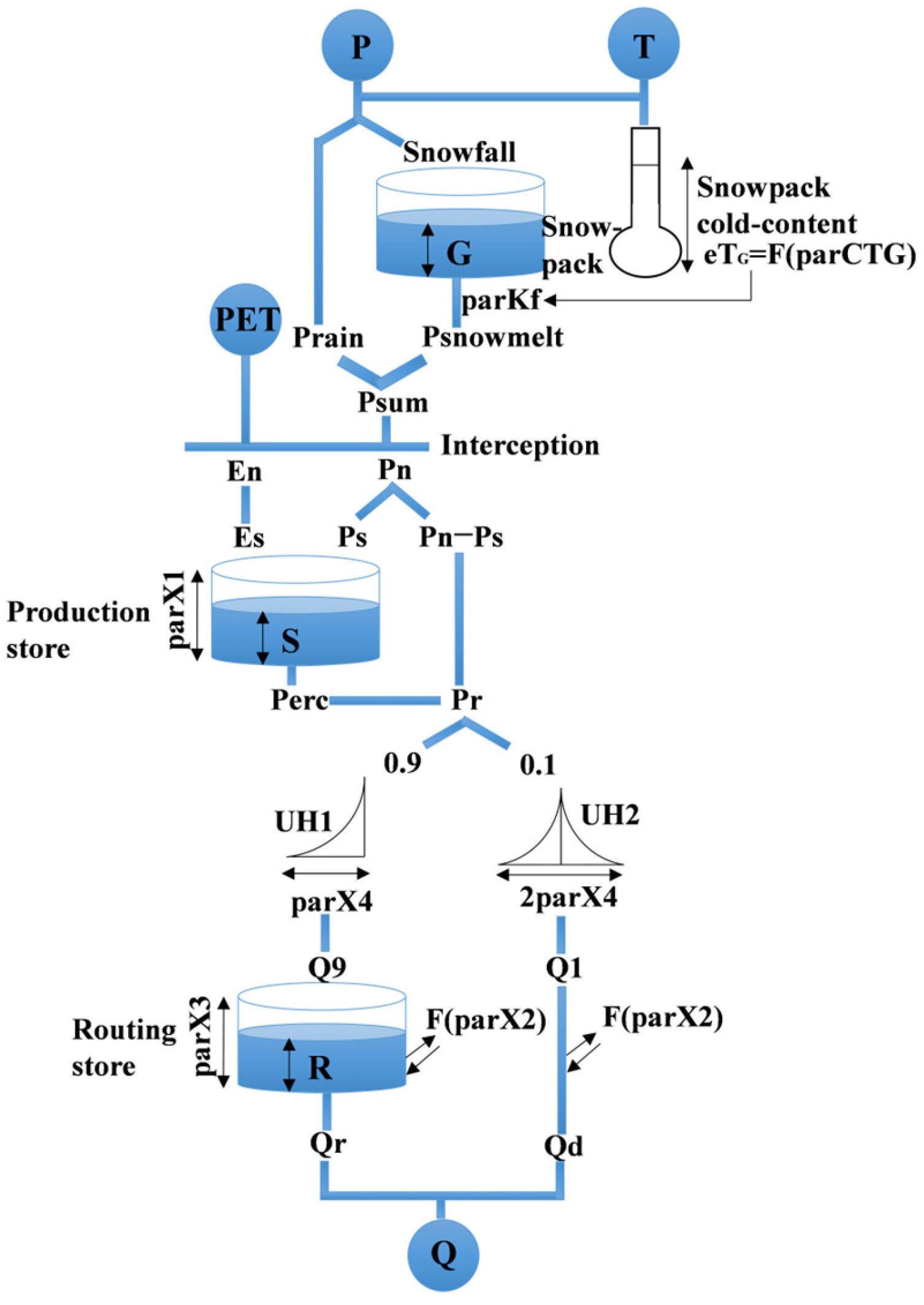
2.2. Hydrological Model

The GR4neige model integrates the GR4J model, which stands for the Génie Rural French model analyzing four parameters on a daily basis with the CemaNeige snow module. The GR4neige model is a lumped conceptual rainfall–runoff hydrological model and has found widespread applicability [5,6,49]. The model contains a simple model structure and merely six model parameters. The GR4neige model takes P, PET, and T as its primary input variables and generates streamflow and ET as outputs. The model structure was described as shown in Figure 2. The model parameters are shown in

Table 1. The notation, definition, and range of parameters in the GR4neige model.

Parameters	Definition	Range
parX1	The maximum capacity of the production store (mm)	100–1200
parX2	Groundwater exchange coefficient (mm)	−5–3
parX3	One day ahead of the maximum capacity of the routing store (mm)	20–300
parX4	Time base of a unit hydrograph UH1 (days)	1.1–2.9
parCTG	Snowpack cold content	0–1
parKf	Degree-day factor (mm/day/°C)	0–10

.

The GR4neige model relies on two stores and a hydrograph-based routing scheme to emulate the rainfall–runoff processes [50]. The two stores consist of the production store and the routing store. The production store incorporates a soil moisture accounting component to determine effective rainfall [51]. The routing store simulates the water exchange process, representing water losses to or acquisitions from deep aquifers [52]. The two flow components are collectively partitioned: 90% of the runoff is directed through a unit hydrograph followed by a non-linear routing reservoir, while the remaining 10% follows a unit hydrograph for routing [3,53]. The maximum capacity of the production store (parX1) has been confirmed as the most sensitive parameter and has the largest influence on model prediction [54]. parX1 controlled the amount of moisture retained by the soil. The process calculation associated with parX1 is as follows:

$$\mathrm{I}\mathrm{f} Pn>0, P_s=\frac{parX1\left(1-{\left(\frac{S}{parX1}\right)}^2\right)\mathit{tanh}\left(\frac{P_n}{parX1}\right)}{1+\frac{S}{parX1}\mathit{tanh}\left(\frac{P_n}{parX1}\right)}$$

(1)

$$\mathrm{I}\mathrm{f} Pn<0 \mathrm{a}\mathrm{n}\mathrm{d} En>0, E_s=\frac{S\left(2-\frac{S}{parX1}\right)\mathit{tanh}\left(\frac{E_n}{parX1}\right)}{1+\left(1-\frac{S}{parX1}\right)\mathit{tanh}\left(\frac{E_n}{parX1}\right)}$$

(2)

where P_n represents net rainfall (mm), E_n is net evapotranspiration capacity (mm), P_s refers to the portion of rainfall that contributes to filling the production store (mm), E_s represents the actual evapotranspiration of the production store (mm), and S is the storage capacity of the production store (mm).

parX1 represents the water storage capacity and is conventionally treated as a time-invariant parameter. However, climate variability and vegetation coverage change may influence the catchment properties and then alter the values of parX1 [24,55]. Other parameters, including groundwater exchange coefficient (parX2), one day ahead of the maximum capacity of the routing store (parX3), time base of a unit hydrograph UH1 (parX4), snowpack cold content (parCTG), and degree-day factor (parKf), are insensitive to climate variability or vegetation coverage [56]. Understanding the time-varying characteristics of parX1 within the GR4neige model is crucial for accurately assessing how the model responds to the changing environment.

2.3. The Long Short-Term Memory Network

The long short-term memory network (LSTM), as a special type of recurrent neural network (RNN), can effectively address the issue of vanishing gradients commonly encountered in traditional RNNs [57]. The LSTM model incorporates three gates that regulate the information flow within the LSTM cell [58]. The first gate, known as the forget gate, regulates the selective retention or discarding of information from the cell [59]. The second gate is the input gate that dictates the extent to which incoming data contributes to updating the cell state at the present time step [60]. The third gate, referred to as the output gate, exercises control over transferring cell state information to the new hidden state [61]. The LSTM model is calculated as follows:

$$\mathrm{F}\mathrm{o}\mathrm{r}\mathrm{g}\mathrm{e}\mathrm{t} \mathrm{gate}: f_t=\sigma \left(W_f{x}_t+U_f{h}_{t-1}+b_f\right)$$

(3)

$$\mathrm{P}\mathrm{o}\mathrm{t}\mathrm{e}\mathrm{n}\mathrm{t}\mathrm{i}\mathrm{a}\mathrm{l} \mathrm{c}\mathrm{e}\mathrm{l}\mathrm{l} \mathrm{s}\mathrm{t}\mathrm{a}\mathrm{t}\mathrm{e}: \tilde{c}=\mathit{tanh}(W_{\tilde{c}}{x}_t+U_{\tilde{c}}{h}_{t-1}+b_{\tilde{c}})$$

(4)

$$\mathrm{I}\mathrm{n}\mathrm{p}\mathrm{u}\mathrm{t} \mathrm{g}\mathrm{a}\mathrm{t}\mathrm{e}: i_t=\sigma (W_i{x}_t+U_i{h}_{t-1}+b_i)$$

(5)

$$\mathrm{C}\mathrm{e}\mathrm{l}\mathrm{l} \mathrm{s}\mathrm{t}\mathrm{a}\mathrm{t}\mathrm{e}: c_t=f_t\odot c_{t-1}+i_t\odot \tilde{c}$$

(6)

$$\mathrm{O}\mathrm{u}\mathrm{t}\mathrm{p}\mathrm{u}\mathrm{t} \mathrm{g}\mathrm{a}\mathrm{t}\mathrm{e}: o_t=\sigma (W_o{x}_t+U_o{h}_{t-1}+b_o)$$

(7)

$$\mathrm{H}\mathrm{i}\mathrm{d}\mathrm{d}\mathrm{e}\mathrm{n} \mathrm{s}\mathrm{t}\mathrm{a}\mathrm{t}\mathrm{e}:{ h}_t=\mathit{tanh}(c_t)\odot o_t$$

(8)

where $i_t$, $f_t$, and $o_t$ represent three gates, including the input, forget, and output gates, respectively, $\sigma (\cdot )$ and $tanh\left(\cdot \right)$ are logistic sigmoid and hyperbolic tangent functions, respectively, $\odot$ signifies element-wise multiplication, $W_f$, $W_{\tilde{c}}$, $W_i$, $W_o$, $U_f$, $U_{\tilde{c}}$, $U_i$, and $U_o$ represent the gate-specific network weights, and $b_f$, $b_{\tilde{c}}$, $b_i$, and $b_o$ are the gate-specific network bias parameters

This comprehensive gating structure enables the LSTM model to preserve and manipulate information over extended sequences, making it particularly adept at capturing intricate temporal dependencies. Consequently, this approach has achieved broad applicability within the hydrology domain [62,63,64,65,66]. This study employed the LSTM model to construct a parameter network mapping relationship between input data and parameters.

2.4. Differentiable Parameter Learning

We implemented the GR4neige model in PyTorch and integrated it with dPL as a regionalized parameterization scheme. The dPL incorporates a global constraint by defining the loss function over the entire training dataset for training such a map. We built two distinct networks, including static and dynamic parameter networks (Figure 3). Firstly, we constructed a dynamic parameter network designed to capture the time-varying features of parX1. Simultaneously, we built a static parameter network for a time-invariant parX1, enabling a comparison with the dynamic parameter network and facilitating an assessment of the advantages of the dynamic parameter network improvements.

We trained a static parameter network (g_A) that mapped static attributes (A) (Table S1) to physical model parameters (θ) using Equation (9). The network structure adopted a multilayer perceptron network. In the static parameter network, the six parameters of the GR4neige model were treated as constants. Additionally, we trained a dynamic parameter network (g_Z) to map static attributes (A) and dynamic features, including meteorological elements, soil moisture, and vegetation growth (x_t), to the physical model parameters (θ_t) following the procedures defined in Equation (10). For the dynamic parameter network, parX1 was treated as time-varying, while the other five parameters were assumed to be constant over time. The LSTM model was used to build the dynamic parameter network and can produce temporal sequences. The stationary parameters across different periods do not entail circular logic or information leakage, as the differentiable physical model ensures that only appropriate parameter values lead to a reasonable loss [33]. The time-invariant parameters were exclusively extracted at the final time step, while the time-varying parameter received new values daily.

$${\theta }^i={\mathrm{g}}_{\mathrm{A}}\left({\mathrm{A}}^{\mathrm{i}}\right)$$

(9)

$${\theta }_t^i={\mathrm{g}}_{\mathrm{Z}}({\mathrm{A}}^{\mathrm{i}},x_t^i)$$

(10)

Since parX1 is sensitive to meteorological and vegetation conditions, we selected several relevant data types. PET, P, and T represent meteorological conditions [67]. The NDVI serves as an indicator of vegetation growth status [68]. SM significantly influences the land surface fluxes of the water and energy balances [69,70,71]. Therefore, the abovementioned five input features were used to build parameter models. To evaluate the influence of different input features on the performance of dPL, we first assessed the time-varying parameter model using each of the five features, and then we tested the model using all five types of data simultaneously. The tested cases are listed in

Table 2. The tested cases in this study.

Case	Input Data
gA	Static attributes
gZ,1	Static attributes + PET
gZ,2	Static attributes + P
gZ,3	Static attributes + T
gZ,4	Static attributes + SM
gZ,5	Static attributes + NDVI
gZ,6	Static attributes + PET + P + T + SM + NDVI

.

The training and evaluation periods spanned from 2003 to 2008 and 2009 to 2012, respectively. We used 256 hidden sizes and a batch size comprising 200 instances. The training instances had a length of 365 days. The loss function incorporated the Nash–Sutcliffe efficiency (NSE), a widely adopted metric for assessing hydrological modeling performance.

$$\mathrm{N}\mathrm{S}\mathrm{E}=1-\frac{{\sum }_{i-1}^n(Q_{obs}-Q_{sim}{)}^2}{{\sum }_{i-1}^n(Q_{obs}-\overline{Q_{obs}}{)}^2}$$

(11)

where $Q_{obs}$ signifies the observed values, $Q_{sim}$ represents simulated values, $\overline{Q_{obs}}$ denotes the mean observed value, and n represents the overall count of data values.

2.5. The Empirical Function Method

We adopted the function forms proposed by Pan et al. [72], which have shown good performance in the central United States. The function forms considered the seasonal and long-term variability. The seasonal variations in attributes of the catchment are accounted for by adjusting parX1 based on a sine function with an annual cycle (365 days), characterized by its amplitude and phase [24]. Catchment response undergoes long-term changes delineated by a linear trend in parX1. The time-varying function form for parX1 is given as

$$parX1={\alpha }_1+a_{2}t+a_3\mathit{sin}\left(2\pi \frac{a_4+t}{365}\right)$$

(12)

where t represents the duration in days, α₁ represents the constant, α₂ signifies the linear trend, α₃ represents the amplitude, and α₄ signifies the phase of the sine component.

2.6. The Evaluation Metrics

In this study, we considered two evaluation metrics to assess streamflow accuracy: Pearson’s correlation (Corr) and NSE. Corr evaluates the linear correlation coefficient between simulated and observed values [73]. NSE quantifies the degree of deviation between the measured and simulated values, ranging from negative infinity to 1. The equation for Corr is shown as follows:

$$\mathrm{Corr}=\frac{{\sum }_{\mathrm{i}-1}^n\left(Q_{obs}-\overline{Q_{obs}}\right)\left(Q_{\mathit{sim}}-\overline{Q_{\mathit{sim}}}\right)}{\sqrt{{\sum }_{\mathrm{i}-1}^n{\left(Q_{obs}-\overline{Q_{obs}}\right)}^2}\sqrt{{\sum }_{\mathrm{i}-1}^n{\left(Q_{\mathit{sim}}-\overline{Q_{\mathit{sim}}}\right)}^2}}$$

(13)

where $\overline{Q_{\mathit{sim}}}$ represents the mean simulated value.

3. Results

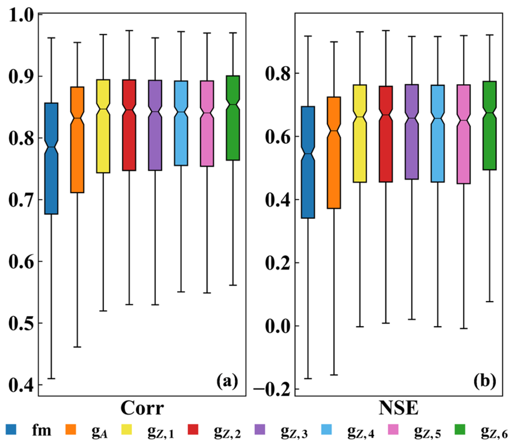
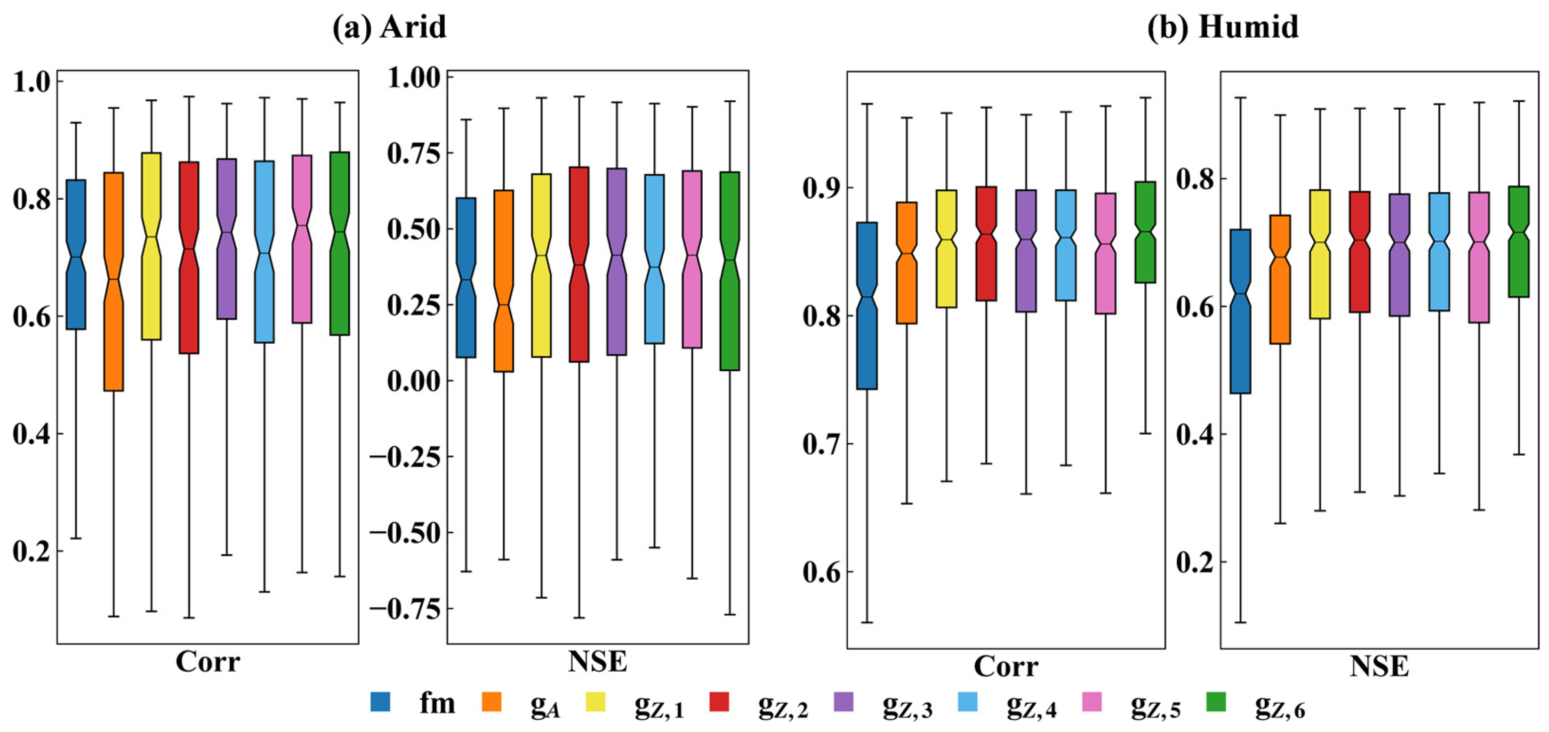
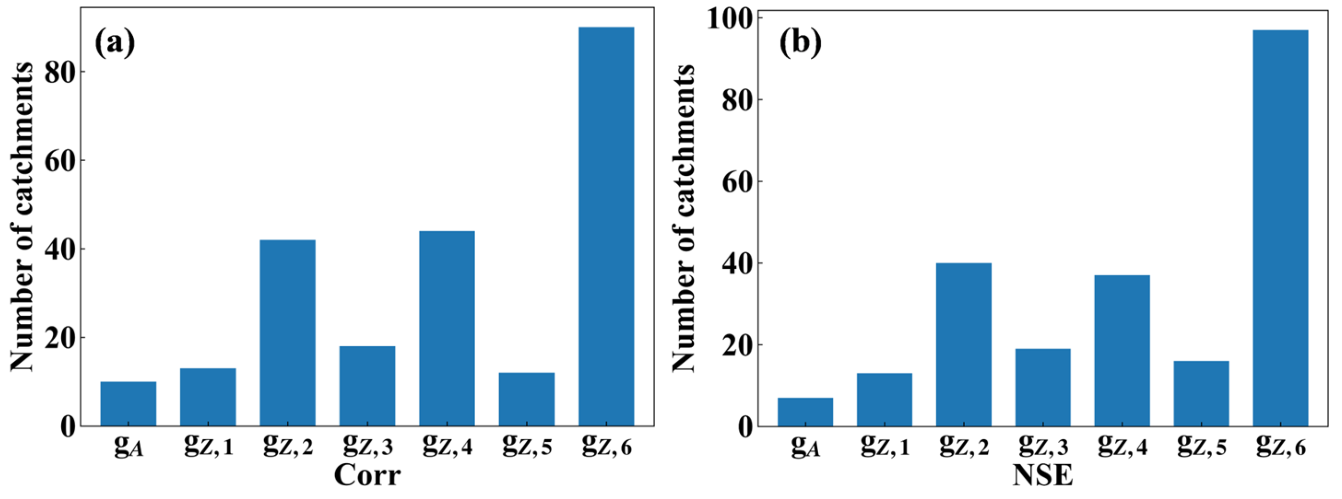
3.1. The Accuracy of Streamflow Estimation

The six scenarios of the dynamic parameter network outperformed the static parameter network, with the median Corr and NSE increasing by ranges of 0.008 to 0.022 and 0.033 to 0.057, respectively (Figure 4). Among the six scenarios of the dynamic parameter network, g_Z,6 exhibited the most significant advantage, with a median Corr of 0.854 and a median NSE of 0.675, respectively. It indicated that employing time-varying parameters has the potential to enhance the model accuracy compared to using time-invariant parameters. The dynamic components within hydrological models are often oversimplified owing to an inadequate understanding of their underlying hydrological processes [74,75,76]. Time-varying parameters have the potential to rectify the structural deficiencies inherent in traditional hydrological models of time-invariant parameters. Moreover, dPL had better performance than the empirical fm, with an increase in Corr and NSE by 0.055 and 0.114, respectively, in g_Z,6. This suggests that dPL can extract more information from the relationships between parameters and inputs than the empirical fm.

We conducted a comparative analysis of the streamflow accuracy of the empirical fm and dPL involving static and dynamic parameter networks across different climate zones (Figure 5). Notably, model accuracy was higher in humid catchments than in arid catchments for both dPL and the empirical fm. The highly accurate streamflow estimation in arid catchments is challenging due to the impact of short-duration, high-intensity rainfall events that are not accounted for in daily precipitation records, leading to the omission of peak events [77,78,79]. In arid catchments, the empirical fm surpassed the static parameter network but still lagged behind the six scenarios of the dynamic parameter network (Figure 5a). The accuracy of streamflow simulation in the six scenarios of the dynamic parameter network improved when considering a single dynamic input feature compared to incorporating five dynamic input features simultaneously. In the six scenarios of the dynamic parameter network, g_z,1, g_z,3, and g_z,5 outperformed g_z,6. We selected some arid catchments and observed an underestimation phenomenon for peak flow in g_z,1, g_z,3, g_z,5, and g_z,6 (see the circled part in Figure S2). Compared with g_z,6, the three dPL models, including g_z,1, g_z,3, and g_z,5, effectively alleviated the underestimation of peak flow. In humid catchments, both the static and dynamic parameter networks demonstrated superior performance compared to the empirical fm (Figure 5b). The six scenarios of the dynamic parameter network all outperformed the static parameter network. g_z,6 exhibited significant performance superiority over other scenarios of the dynamic parameter network. The accuracy of streamflow simulation was higher when simultaneously considering five dynamic input features than a single dynamic input feature.

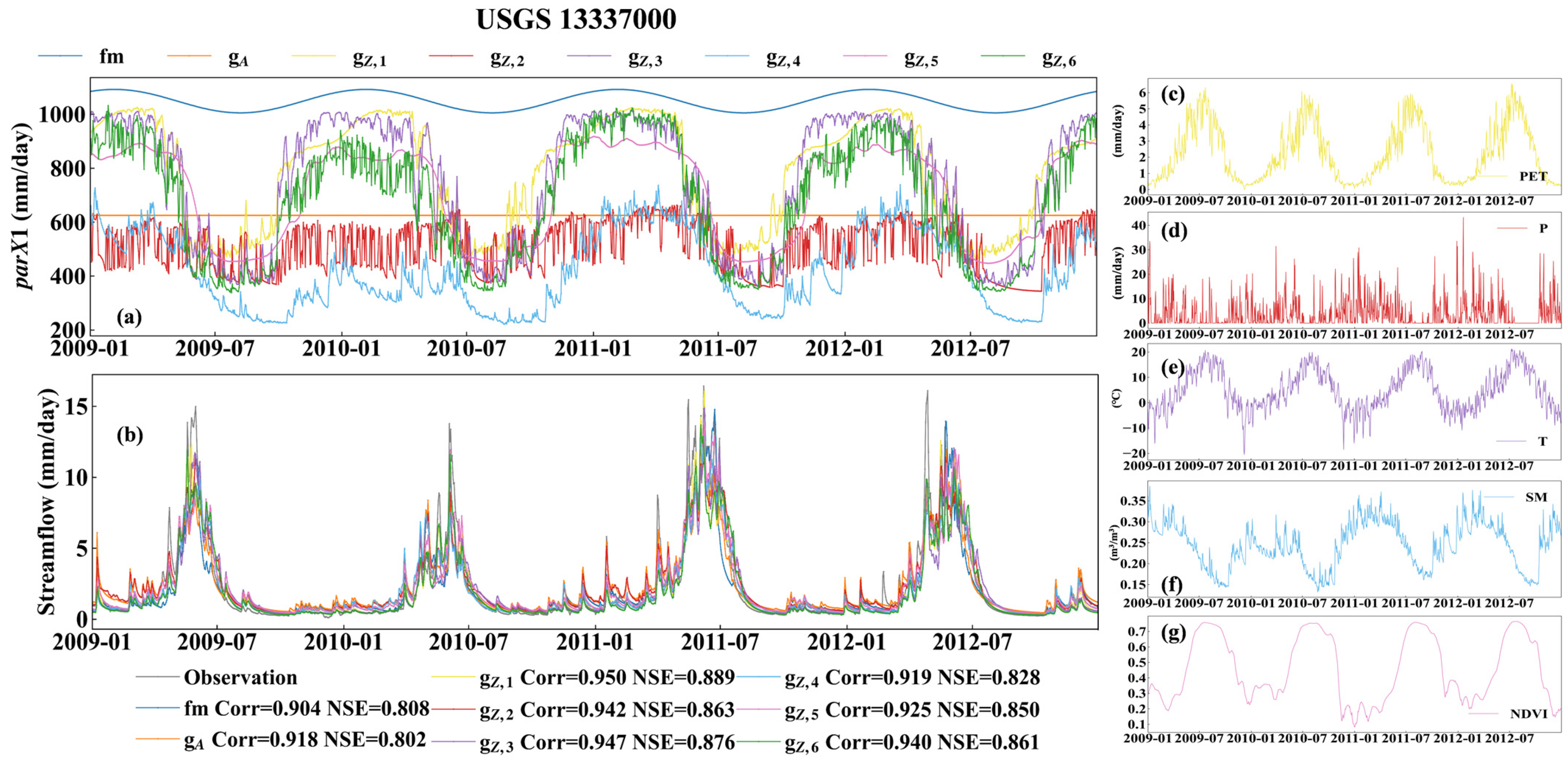
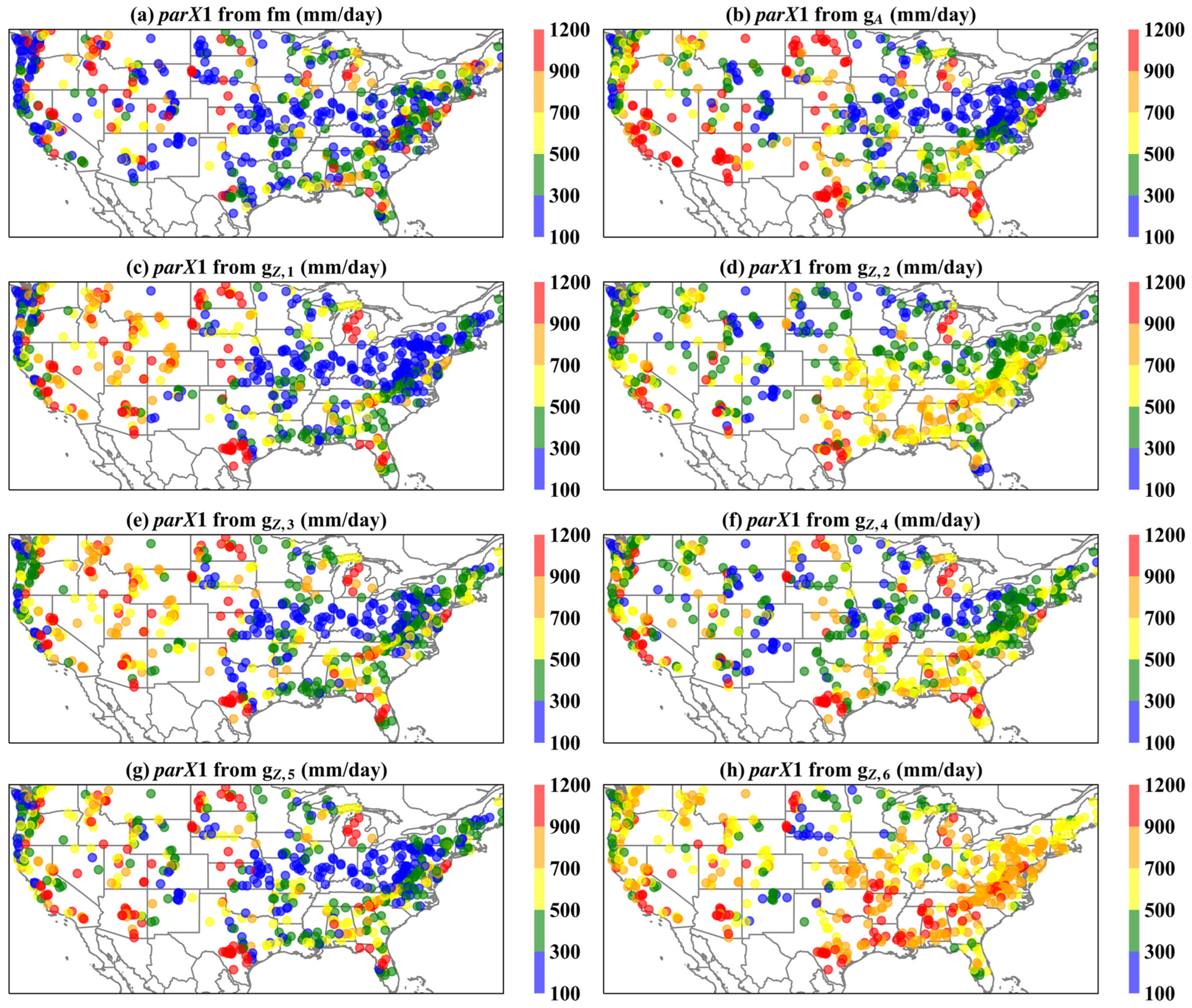
3.2. The Spatiotemporal Variation Characteristics of parX1

We selected three catchments to analyze the spatiotemporal variation characteristics of parX1 (Figure S3). Among these three catchments, one catchment has the USGS 02137727 station as the outlet and is located in the humid zone. The other two catchments, with USGS 13337000 and USGS 13340000 stations as the outlets, are situated in the arid zone, and these two arid catchments are adjacent. We analyzed time-varying parX1 within different climate zones and adjacent catchments. parX1 obtained from the empirical fm and six scenarios of the dynamic parameter network showed significant differences in temporal variability. parX1 displayed a periodic change in the empirical fm and six scenarios of the dynamic parameter network in three catchments, except for g_z,2 in the three catchments and g_z,4 in the humid catchment (Figure 6a, Figure 7a and Figure 8a). parX1 obtained from g_z,2 in three catchments and g_z,4 in the humid catchment showed little monthly variation. The periodic change within the empirical fm and smoother curve were easily explained by its functional form, which incorporates sinusoidal and linear components. However, dPL was not given a specific functional form and captured a periodic pattern from the input and parameters. PET, T, and the NDVI showed a periodic change and had a negative correlation with parX1. The highest values of parX1 occurred in late winter or early spring, while the lowest values were observed in the summer. Westra et al. [24] found that periodic variations in parX1 can improve model accuracy. Pan et al. [80] showed that the mean period of parX1 was 26.2–46.3. They suggested that the fluctuation in parX1 exhibited periodic variations, potentially attributed to the seasonal growth and the wilting of vegetation. The two adjacent arid catchments are predominantly characterized by evergreen needleleaf forests and have relatively high elevations and steep slopes. The main reason for the decrease in parX1 was the increased surface runoff in catchments with high altitudes and steep slopes, leading to low soil water retention. This situation subjects vegetation to prolonged drought stress, significantly impacting the survival and the growth of plants. Pan et al. [81] also found that the decrease in parX1 was associated with high elevation and high vegetation coverage during drought occurrences. The humid catchment is primarily covered by mixed forests and has substantial snowfall during the winter. Higher values of parX1 were observed in late winter/early spring. This could be because plants are in a dormant state during the winter, resulting in relatively low water consumption, and the snowfall stored in the soil increases parX1. In the summer, as plants grow, water consumption increases, leading to a subsequent decrease in parX1. The two adjacent catchments with the USGS 13337000 and USGS 13340000 stations as the outlet have similar climate conditions and vegetation types. Adjacent catchments share similar climatic and geological characteristics, resulting in the similarity of parX1 [15]. parX1 from six scenarios of the dynamic parameter network showed similarities in both catchments, while those from the empirical fm exhibited significant differences (Figure 7a and Figure 8a). The parameter found by six scenarios of the dynamic parameter network seems more coherent with spatial clusters than those from the empirical fm.

We compared the spatiotemporal variation characteristics of parX1 derived from the empirical fm and dPL. The estimated daily mean parX1 is shown in Figure 9. These two methods exhibited differences in the magnitude and spatial distribution of the daily mean parX1. It is seen that the daily mean parX1 calculated by the empirical fm was the lowest, while that from g_Z,6 was the highest. The daily mean parX1 from the empirical fm mainly ranged from 100 to 300 mm/day, with higher parX1 in the southeast and northwest regions (Figure 9a). The daily mean parX1 from g_z,6 mainly ranged from 700 to 900 mm/day (Figure 9h). It was higher in most of the southeast regions and sporadic southwest regions. The daily mean parX1 obtained from dPL generally exhibited a similar spatial distribution, except for the central and eastern regions. In these specific regions, the g_A, g_z,1, g_z,3, and g_z,5 exhibited low parX1 (ranging from 100 to 300 mm/day), while g_z,2, g_z,4, and g_z,6 showed high parX1 (mainly ranging from 300 to 900 mm/day). The estimated daily mean parX1 from dPL displayed a distinct geographical clustering pattern compared to the empirical fm, especially in the southeast and northwest regions. The empirical fm is calibrated for each catchment individually and thus cannot exploit the parameter spatial cluster. In contrast, dPL uses the global constraint to learn the parameter spatial cluster. Therefore, dPL provided a more comprehensive and effective approach for capturing spatial patterns in parameter clusters (Figure 9b–h), allowing for a holistic understanding of the interdependencies and variations in parX1 across different geographical regions.

3.3. Model Performance in ET Estimation

A well-calibrated hydrology model may exhibit a pseudo-accurate, equifinal model that provides the right answers for the wrong reasons [82]. We validated the uncalibrated ET variables to check whether the intermediate physical process can be learned. LSTM is a black-box model and only predicts the object variable. dPL coupling the conceptual hydrological model and data-driven model has a physical mechanism and better interpretability. dPL obtains parameter estimation and simulates the hydrology process, including the object variable and uncalibrated intermediate variable. We compared the ET accuracy of the empirical fm and dPL of the static and dynamic parameter networks using Corr. The results showed that dPL outperformed the empirical fm, as shown in Figure 10. g_z,6 achieved the most significant improvement compared to the empirical fm, with a Corr increase of 0.053. The empirical fm underestimated ET values, and g_z,6 improved this issue (results not presented). The dynamic parameter network, including g_z,2, g_z,5, and g_z,6, surpassed the static parameter network with respect to ET estimation.

4. Discussion

4.1. The Spatial Variability of parX1

parX1 obtained with dPL and the empirical fm exhibited significant spatial variation. Moreover, parX1 estimated by dPL demonstrated apparent spatial clustering compared to that estimated by the empirical fm. We applied Corr to analyze the correlation between the daily mean parX1 obtained with static and dynamic parameter networks and covariates and further explored the reason for the spatial variation characteristics of parX1 (Figure 11). Corr values of ≤0.39 indicate a weak correlation, 0.40–0.69 suggest a moderate correlation, and 0.70–1.0 signify a strong correlation [83]. The daily mean parX1 obtained from static and dynamic parameter networks exhibited positive correlations with low_prec_dur, aridity, low_prec_freq, geol_permeability, pet_mean, high_prec_freq, and dom_land_cover. Weak positive correlations were observed between the daily mean parX1 and covariates, except in a few scenarios. In g_A, the daily mean parX1 had a moderate positive correlation with low_prec_dur, high_prec_dur, aridity, and low_prec_freq (Figure 11a). The daily mean parX1 obtained from g_z,1 showed a moderate positive correlation with aridity, high_prec_dur, and low_prec_dur (Figure 11b). The daily mean parX1 obtained from static and dynamic parameter networks showed a negative correlation with silt_frac, max_water_content, soil_depth_statsgo, dom_land_cover_frac, and p_seasonality. In most cases, there were weak negative correlations between the daily mean parX1 and covariates. The daily mean parX1 obtained from g_A exhibited a moderate negative correlation with silt_frac, gvf_diff, lai_diff, and gvf_max (Figure 11a). In g_z,1, the daily mean parX1 had a moderate negative correlation with gvf_max, lai_diff, silt_frac, lai_max, and gvf_diff (Figure 11b). The daily mean parX1 obtained from g_z,3 and g_z,5 showed a moderate correlation with silt_frac (Figure 11d,f).

The daily mean parX1 obtained from static and dynamic parameter networks exhibited similar spatial distributions, except in the central and eastern regions. The daily mean parX1 obtained from g_A, g_z,1, g_z,3, and g_z,5 ranged from 100 to 300 mm/day in the central and eastern regions. In g_A, g_z,1, g_z,3, and g_z,5, the daily mean parX1 had a moderate negative correlation with the silt fraction. In the central and eastern regions, the silt fraction exceeded 40% (Figure S1f). Since parX1 represents the water storage capacity, the catchment with a higher silt fraction had low water retention and, consequently, led to lower parX1. In contrast, g_z,2, g_z,4, and g_z,6 had an obviously higher parX1 than g_A, g_z,1, g_z,3, and g_z,5. In g_z,2, g_z,4, and g_z,6, the daily mean parX1 had a weak correlation with each covariate. g_z,2, g_z,4, and g_z,6 considered the effect of SM or/and P on parX1. It is seen in Figure S1b,d that the central and eastern regions have abundant rainfall and higher surface soil moisture. Abundant rainfall and higher surface soil moisture, as well as smaller slopes, in the central and eastern regions potentially lead to larger water storage capacity and larger parX1. We further assessed the accuracy of streamflow simulations in 229 catchments where the silt fraction exceeds 40%. Most of these catchments are located in the central and eastern regions (Figure S1f). The highest proportional quantities of optimal streamflow simulation precision were achieved by g_z,6, followed by g_z,2 and g_z,4, and then g_z,3, g_z,1, g_z,5, and g_A (Figure 12). It is also found that the silt fraction had a stronger negative correlation with parX1 in g_A, g_z,1, g_z,3, and g_z,5, while such correlation did not exist in g_z,2, g_z,4, and g_z,6. The results indicated abundant rainfall and higher surface soil moisture had greater impacts on parX1 than soil properties, such as the silt fraction, in the central and eastern regions.

4.2. The Limitation of This Study

This study has several limitations. Firstly, dPL of static and dynamic parameter networks had better performance than the empirical fm in streamflow and ET estimation. Nonetheless, an overparameterization issue was evident within dPL. The six scenarios of the dynamic parameter network outperformed the static parameter network in streamflow estimation, while the dynamic parameter network in scenarios g_z,1, g_z,3, and g_z,5 exhibited lower accuracy in ET compared to the static parameter network. The overparameterization issue has persistently existed during parameter calibration [84,85]. This study primarily focused on the impact of time-varying parameters on streamflow accuracy and did not delve into the underlying reasons for the overparameterization issue. Secondly, we observed that in arid and humid catchments, the same type of input data (or their combination) contributed differently to streamflow estimation in the framework of dPL. This study provided limited insights into the inner mechanism of this phenomenon. Further studies should explore the interpretability of the parameter network to analyze how the input factors cause the spatiotemporal variability of parX1. Thirdly, we only considered the influence of climate factors, soil conditions, and vegetation change on the time-varying parameters. Human activities, such as dam construction and irrigation, may also yield time-varying parameters [86]. More data and new methods are required to understand the induced temporal variabilities of parameters.

5. Conclusions

The parameters of the conceptual hydrological model exhibit time-varying features in a changing environment. The GR4J-CemaNeige coupling model (GR4neige) was selected due to its simple structure and merely six parameters. The maximum capacity of the production store (parX1) is the most sensitive parameter in the GR4neige model and represents the catchment water storage capacity. This study applied differentiable parameter learning (dPL) to construct a neural network-based parameter module and identify the time-varying parX1 in the GR4neige model. Two types of dPL were built, including static and dynamic parameter networks, to assess the advantages of time-varying parameters. In dynamic parameter networks, we considered the influence of climate factors, soil conditions, and vegetation change on the performance of dPL. The dPL was compared with the empirical functional method (fm) to analyze the strengths and limitations of dPL. Both dPL and the empirical fm were applied to 671 catchments in the United States to test the model accuracy and investigate the spatiotemporal variation characteristics of parX1. The main findings are listed as follows:

(1)

The dPL of static and dynamic parameter networks achieved good performance for streamflow estimation. The six scenarios of the dynamic parameter network significantly outperformed the static parameter network. It was demonstrated that time-varying parameters can enhance the accuracy of streamflow estimation compared to time-invariant parameters.

(2)

There were differences in streamflow estimation among the dynamic parameter network driven by distinct input features in humid and arid catchments. In humid catchments, simultaneously incorporating all five factors, including PET, P, T, SM, and the NDVI, achieved optimal streamflow simulation. In arid catchments, it was preferable to introduce PET, T, and the NDVI separately for improved performance.

(3)

The dPL outperformed the empirical fm in both streamflow and intermediate variable (ET) estimation. parX1 generated by both the dynamic parameter network and the empirical fm showed significant spatiotemporal variation. However, parX1 estimated by the dynamic parameter networks showed obvious spatial clustering across 671 catchments within the United States compared to that estimated by the empirical fm. The time-varying parX1 showed a periodic change and had a negative correlation with PET, T, and the NDVI. The spatial variation of parX1 was more susceptible to P and SM in the central and eastern catchments.

These findings offer valuable insights into the potential of dPL for enhancing streamflow estimation accuracy and understanding the spatiotemporal variations in the time-varying parX1 within hydrological models.

References

1. Bergström, S.; Rapporter, S. Development and Application of a Conceptual Runoff Model for Scandinavian Catchments; SMHI: Norrköping, Sweden, 1976; Volume 7. [Google Scholar]
2. Seibert, J.; Vis, M.J.P. Teaching Hydrological Modeling with a User-Friendly Catchment-Runoff-Model Software Package. Hydrol. Earth Syst. Sci. 2012, 16, 3315–3325. [Google Scholar] [CrossRef]
3. Perrin, C.; Michel, C.; Andréassian, V. Improvement of a Parsimonious Model for Streamflow Simulation. J. Hydrol. 2003, 279, 275–289. [Google Scholar] [CrossRef]
4. Zhao, R. The Xinanjiang Model Applied in China. J. Hydrol. 1992, 135, 371–381. [Google Scholar] [CrossRef]
5. Qi, W.; Chen, J.; Li, L.; Xu, C.; Li, J.; Xiang, Y.; Zhang, S. A Framework to Regionalize Conceptual Model Parameters for Global Hydrological Modeling. Hydrol. Earth Syst. Sci. Discuss. 2020, 2020, 1–28. [Google Scholar] [CrossRef]
6. Reichert, P.; Ma, K.; Höge, M.; Fenicia, F.; Baity-jesi, M.; Feng, D.; Shen, C. Metamorphic Testing of Machine Learning and Conceptual Hydrologic Models. Hydrol. Earth Syst. Sci. Discuss. 2023, 2023, 1–37. [Google Scholar] [CrossRef]
7. Arsenault, R.; Martel, J.L.; Brunet, F.; Brissette, F.; Mai, J. Continuous Streamflow Prediction in Ungauged Basins: Long Short-Term Memory Neural Networks Clearly Outperform Traditional Hydrological Models. Hydrol. Earth Syst. Sci. 2023, 27, 139–157. [Google Scholar] [CrossRef]
8. Baez-Villanueva, O.M.; Zambrano-Bigiarini, M.; Mendoza, P.A.; McNamara, I.; Beck, H.E.; Thurner, J.; Nauditt, A.; Ribbe, L.; Thinh, N.X. On the Selection of Precipitation Products for the Regionalisation of Hydrological Model Parameters. Hydrol. Earth Syst. Sci. 2021, 25, 5805–5837. [Google Scholar] [CrossRef]
9. Beven, K. A Manifesto for the Equifinality Thesis. J. Hydrol. 2006, 320, 18–36. [Google Scholar] [CrossRef]
10. Gan, Y.; Duan, Q.; Gong, W.; Tong, C.; Sun, Y.; Chu, W.; Ye, A.; Miao, C.; Di, Z. A Comprehensive Evaluation of Various Sensitivity Analysis Methods: A Case Study with a Hydrological Model. Environ. Model. Softw. 2014, 51, 269–285. [Google Scholar] [CrossRef]
11. Yang, W.; Xia, R.; Chen, H.; Wang, M.; Xu, C.Y. The Impact of Calibration Conditions on the Transferability of Conceptual Hydrological Models under Stationary and Nonstationary Climatic Conditions. J. Hydrol. 2022, 613, 128310. [Google Scholar] [CrossRef]
12. Wang, Y.; Peng, T.; Lin, Q.; Singh, V.P.; Dong, X.; Chen, C.; Liu, J.; Chang, W.; Wang, G. A New Non-Stationary Hydrological Drought Index Encompassing Climate Indices and Modified Reservoir Index as Covariates. Water Resour. Manag. 2022, 36, 2433–2454. [Google Scholar] [CrossRef]
13. Arnaud, P.; Bouvier, C.; Cisneros, L.; Dominguez, R. Influence of Rainfall Spatial Variability on Flood Prediction. J. Hydrol. 2002, 260, 216–230. [Google Scholar] [CrossRef]
14. Morozov, E.; Zavialov, P.; Zamshin, V.; Moller, O.; Frey, D.; Zuev, O.; Seliverstova, A.; Bulanov, A.; Lipinskaya, N.; Salyuk, P.; et al. Spreading of the Amazon River Plume. Russ. J. Earth Sci. 2023, 23, 1–18. [Google Scholar] [CrossRef]
15. Xiong, M.; Liu, P.; Cheng, L.; Deng, C.; Gui, Z.; Zhang, X.; Liu, Y. Identifying Time-Varying Hydrological Model Parameters to Improve Simulation Efficiency by the Ensemble Kalman Filter: A Joint Assimilation of Streamflow and Actual Evapotranspiration. J. Hydrol. 2019, 568, 758–768. [Google Scholar] [CrossRef]
16. Legesse, D.; Vallet-Coulomb, C.; Gasse, F. Hydrological Response of a Catchment to Climate and Land Use Changes in Tropical Africa: Case Study South Central Ethiopia. J. Hydrol. 2003, 275, 67–85. [Google Scholar] [CrossRef]
17. Brown, A.E.; Zhang, L.; McMahon, T.A.; Western, A.W.; Vertessy, R.A. A Review of Paired Catchment Studies for Determining Changes in Water Yield Resulting from Alterations in Vegetation. J. Hydrol. 2005, 310, 28–61. [Google Scholar] [CrossRef]
18. Merz, R.; Parajka, J.; Blöschl, G. Time Stability of Catchment Model Parameters: Implications for Climate Impact Analyses. Water Resour. Res. 2011, 47, 1–17. [Google Scholar] [CrossRef]
19. Zhang, X.; Liu, P. A Time-Varying Parameter Estimation Approach Using Split-Sample Calibration Based on Dynamic Programming. Hydrol. Earth Syst. Sci. 2021, 25, 711–733. [Google Scholar] [CrossRef]
20. Krapu, C.; Borsuk, M. A Differentiable Hydrology Approach for Modeling With Time-Varying Parameters. Water Resour. Res. 2022, 58, e2021WR031377. [Google Scholar] [CrossRef]
21. Deng, C.; Liu, P.; Guo, S.; Li, Z.; Wang, D. Identification of Hydrological Model Parameter Variation Using Ensemble Kalman Filter. Hydrol. Earth Syst. Sci. 2016, 20, 4949–4961. [Google Scholar] [CrossRef]
22. Pignotti, G.; Crawford, M.; Han, E.; Williams, M.R.; Chaubey, I. SMAP Soil Moisture Data Assimilation Impacts on Water Quality and Crop Yield Predictions in Watershed Modeling. J. Hydrol. 2023, 617, 129122. [Google Scholar] [CrossRef]
23. Liu, K.; Huang, G.; Šimůnek, J.; Xu, X.; Xiong, Y.; Huang, Q. Comparison of Ensemble Data Assimilation Methods for the Estimation of Time-Varying Soil Hydraulic Parameters. J. Hydrol. 2021, 594, 125729. [Google Scholar] [CrossRef]
24. Westra, S.; Thyer, M.; Leonard, M.; Kavetski, D.; Lambert, M. A Strategy for Diagnosing and Interpreting Hydrological Model Nonstationarity. Water Resour. Res. 2014, 50, 5375–5377. [Google Scholar] [CrossRef]
25. Zhou, L.; Liu, P.; Gui, Z.; Zhang, X.; Liu, W.; Cheng, L.; Xia, J. Diagnosing Structural Deficiencies of a Hydrological Model by Time-Varying Parameters. J. Hydrol. 2022, 605, 127305. [Google Scholar] [CrossRef]
26. Babaeian, E.; Paheding, S.; Siddique, N.; Devabhaktuni, V.K.; Tuller, M. Short- and Mid-Term Forecasts of Actual Evapotranspiration with Deep Learning. J. Hydrol. 2022, 612, 128078. [Google Scholar] [CrossRef]
27. Chen, H.; Huang, J.J.; Dash, S.S.; Wei, Y.; Li, H. A Hybrid Deep Learning Framework with Physical Process Description for Simulation of Evapotranspiration. J. Hydrol. 2022, 606, 127422. [Google Scholar] [CrossRef]
28. Ghobadi, F.; Kang, D. Improving Long-Term Streamflow Prediction in a Poorly Gauged Basin Using Geo-Spatiotemporal Mesoscale Data and Attention-Based Deep Learning: A Comparative Study. J. Hydrol. 2022, 615, 128608. [Google Scholar] [CrossRef]
29. Singh, D.; Vardhan, M.; Sahu, R.; Chatterjee, D.; Chauhan, P.; Liu, S. Machine-Learning- and Deep-Learning-Based Streamflow Prediction in a Hilly Catchment for Future Scenarios Using CMIP6 GCM Data. Hydrol. Earth Syst. Sci. 2023, 27, 1047–1075. [Google Scholar] [CrossRef]
30. Razavi, S. Deep Learning, Explained: Fundamentals, Explainability, and Bridgeability to Process-Based Modelling. Environ. Model. Softw. 2021, 144, 105159. [Google Scholar] [CrossRef]
31. Shu, X.; Ye, Y. Knowledge Discovery: Methods from Data Mining and Machine Learning. Soc. Sci. Res. 2023, 110, 102817. [Google Scholar] [CrossRef]
32. Chen, M.; Qian, Z.; Boers, N.; Jakeman, A.J.; Kettner, A.J.; Brandt, M.; Kwan, M.P.; Batty, M.; Li, W.; Zhu, R.; et al. Iterative Integration of Deep Learning in Hybrid Earth Surface System Modelling. Nat. Rev. Earth Environ. 2023, 4, 568–581. [Google Scholar] [CrossRef]
33. Tsai, W.P.; Feng, D.; Pan, M.; Beck, H.; Lawson, K.; Yang, Y.; Liu, J.; Shen, C. From Calibration to Parameter Learning: Harnessing the Scaling Effects of Big Data in Geoscientific Modeling. Nat. Commun. 2021, 12, 5988. [Google Scholar] [CrossRef] [PubMed]
34. Shen, C.; Appling, A.P.; Gentine, P.; Bandai, T.; Gupta, H.; Tartakovsky, A.; Baity-Jesi, M.; Fenicia, F.; Kifer, D.; Li, L.; et al. Differentiable Modeling to Unify Machine Learning and Physical Models and Advance Geosciences. Nat. Rev. Earth Environ. 2023, 4, 552–567. [Google Scholar] [CrossRef]
35. Feng, D.; Liu, J.; Lawson, K.; Shen, C. Differentiable, Learnable, Regionalized Process-Based Models With Multiphysical Outputs Can Approach State-Of-The-Art Hydrologic Prediction Accuracy. Water Resour. Res. 2022, 58, e2022WR032404. [Google Scholar] [CrossRef]
36. Feng, D.; Beck, H.; Lawson, K.; Shen, C. The Suitability of Differentiable, Physics-Informed Machine Learning Hydrologic Models for Ungauged Regions and Climate Change Impact Assessment. Hydrol. Earth Syst. Sci. 2023, 27, 2357–2373. [Google Scholar] [CrossRef]
37. Yang, W.; Chen, H.; Xu, C.Y.; Huo, R.; Chen, J.; Guo, S. Temporal and Spatial Transferabilities of Hydrological Models under Different Climates and Underlying Surface Conditions. J. Hydrol. 2020, 591, 125276. [Google Scholar] [CrossRef]
38. De Jong, S.M.; Jetten, V.G. Estimating Spatial Patterns of Rainfall Interception from Remotely Sensed Vegetation Indices and Spectral Mixture Analysis. Int. J. Geogr. Inf. Sci. 2007, 21, 529–545. [Google Scholar] [CrossRef]
39. Schoener, G.; Stone, M.C. Impact of Antecedent Soil Moisture on Runoff from a Semiarid Catchment. J. Hydrol. 2019, 569, 627–636. [Google Scholar] [CrossRef]
40. Valéry, A.; Andréassian, V.; Perrin, C. “As Simple as Possible but Not Simpler”: What Is Useful in a Temperature-Based Snow-Accounting Routine? Part 2—Sensitivity Analysis of the Cemaneige Snow Accounting Routine on 380 Catchments. J. Hydrol. 2014, 517, 1176–1187. [Google Scholar] [CrossRef]
41. Addor, N.; Newman, A.J.; Mizukami, N.; Clark, M.P. The CAMELS Data Set: Catchment Attributes and Meteorology for Large-Sample Studies. Hydrol. Earth Syst. Sci. 2017, 21, 5293–5313. [Google Scholar] [CrossRef]
42. Newman, A.J.; Clark, M.P.; Sampson, K.; Wood, A.; Hay, L.E.; Bock, A.; Viger, R.J.; Blodgett, D.; Brekke, L.; Arnold, J.R.; et al. Development of a Large-Sample Watershed-Scale Hydrometeorological Data Set for the Contiguous USA: Data Set Characteristics and Assessment of Regional Variability in Hydrologic Model Performance. Hydrol. Earth Syst. Sci. 2015, 19, 209–223. [Google Scholar] [CrossRef]
43. Sayre, R.; Karagulle, D.; Frye, C.; Boucher, T.; Wolff, N.H.; Breyer, S.; Wright, D.; Martin, M.; Butler, K.; Van Graafeiland, K.; et al. An Assessment of the Representation of Ecosystems in Global Protected Areas Using New Maps of World Climate Regions and World Ecosystems. Glob. Ecol. Conserv. 2020, 21, e00860. [Google Scholar] [CrossRef]
44. Yin, H.; Wang, F.; Zhang, X.; Zhang, Y.; Chen, J.; Xia, R.; Jin, J. Rainfall-Runoff Modeling Using Long Short-Term Memory Based Step-Sequence Framework. J. Hydrol. 2022, 610, 127901. [Google Scholar] [CrossRef]
45. Dorigo, W.; Wagner, W.; Albergel, C.; Albrecht, F.; Balsamo, G.; Brocca, L.; Chung, D.; Ertl, M.; Forkel, M.; Gruber, A.; et al. ESA CCI Soil Moisture for Improved Earth System Understanding: State-of-the Art and Future Directions. Remote Sens. Environ. 2017, 203, 185–215. [Google Scholar] [CrossRef]
46. Gruber, A.; Dorigo, W.A.; Crow, W.; Wagner, W. Triple Collocation-Based Merging of Satellite Soil Moisture Retrievals. IEEE Trans. Geosci. Remote Sens. 2017, 55, 6780–6792. [Google Scholar] [CrossRef]
47. Lian, X.; Hu, X.; Bian, J.; Shi, L.; Lin, L.; Cui, Y. Enhancing Streamflow Estimation by Integrating a Data-Driven Evapotranspiration Submodel into Process-Based Hydrological Models. J. Hydrol. 2023, 621, 129603. [Google Scholar] [CrossRef]
48. Jung, M.; Koirala, S.; Weber, U.; Ichii, K.; Gans, F.; Camps-Valls, G.; Papale, D.; Schwalm, C.; Tramontana, G.; Reichstein, M. The FLUXCOM Ensemble of Global Land-Atmosphere Energy Fluxes. Sci. Data 2019, 6, 74. [Google Scholar] [CrossRef]
49. Shen, H.; Tolson, B.A.; Mai, J. Time to Update the Split-Sample Approach in Hydrological Model Calibration. Water Resour. Res. 2022, 58, e2021WR031523. [Google Scholar] [CrossRef]
50. Cantoni, E.; Tramblay, Y.; Grimaldi, S.; Salamon, P.; Dakhlaoui, H.; Dezetter, A.; Thiemig, V. Hydrological Performance of the ERA5 Reanalysis for Flood Modeling in Tunisia with the LISFLOOD and GR4J Models. J. Hydrol. Reg. Stud. 2022, 42, 101169. [Google Scholar] [CrossRef]
51. Le Moine, N.; Andréassian, V.; Mathevet, T. Confronting Surface- and Groundwater Balances on the La Rochefoucauld-Touvre Karstic System (Charente, France). Water Resour. Res. 2008, 44, W03403. [Google Scholar] [CrossRef]
52. Oudin, L.; Perrin, C.; Mathevet, T.; Andréassian, V.; Michel, C. Impact of Biased and Randomly Corrupted Inputs on the Efficiency and the Parameters of Watershed Models. J. Hydrol. 2006, 320, 62–83. [Google Scholar] [CrossRef]
53. Tian, Y.; Xu, Y.P.; Zhang, X.J. Assessment of Climate Change Impacts on River High Flows through Comparative Use of GR4J, HBV and Xinanjiang Models. Water Resour. Manag. 2013, 27, 2871–2888. [Google Scholar] [CrossRef]
54. Renard, B.; Kavetski, D.; Leblois, E.; Thyer, M.; Kuczera, G.; Franks, S.W. Toward a Reliable Decomposition of Predictive Uncertainty in Hydrological Modeling: Characterizing Rainfall Errors Using Conditional Simulation. Water Resour. Res. 2011, 47, W11516. [Google Scholar] [CrossRef]
55. Zeng, L.; Xiong, L.; Liu, D.; Chen, J.; Kim, J.S. Improving Parameter Transferability of GR4J Model under Changing Environments Considering Nonstationarity. Water 2019, 11, 2029. [Google Scholar] [CrossRef]
56. Tian, J.; Pan, Z.; Liu, P.; Feng, M.; Guo, J. Temporal Variation Scale of the Catchment Water Storage Capacity of 91 MOPEX Catchments. J. Hydrol. Reg. Stud. 2022, 44, 101236. [Google Scholar] [CrossRef]
57. Kratzert, F.; Klotz, D.; Brenner, C.; Schulz, K.; Herrnegger, M. Rainfall—Runoff Modelling Using Long Short-Term Memory (LSTM) Networks. Hydrol. Earth Syst. Sci. 2018, 22, 6005–6022. [Google Scholar] [CrossRef]
58. Kratzert, F.; Klotz, D.; Shalev, G.; Klambauer, G.; Hochreiter, S.; Nearing, G. Towards Learning Universal, Regional, and Local Hydrological Behaviors via Machine Learning Applied to Large-Sample Datasets. Hydrol. Earth Syst. Sci. 2019, 23, 5089–5110. [Google Scholar] [CrossRef]
59. Wei, D.; Wang, B.; Lin, G.; Liu, D.; Dong, Z.; Liu, H.; Liu, Y. Research on Unstructured Text Data Mining and Fault Classification Based on RNN-LSTM with Malfunction Inspection Report. Energies 2017, 10, 406. [Google Scholar] [CrossRef]
60. Sarker, I.H. Deep Learning: A Comprehensive Overview on Techniques, Taxonomy, Applications and Research Directions. SN Comput. Sci. 2021, 2, 420. [Google Scholar] [CrossRef]
61. Zou, Y.; Lin, Z.; Li, D.; Liu, Z.C. Advancements in Artificial Neural Networks for Health Management of Energy Storage Lithium-Ion Batteries: A Comprehensive Review. J. Energy Storage 2023, 73, 109069. [Google Scholar] [CrossRef]
62. Wang, Y.; Huang, Y.; Xiao, M.; Zhou, S.; Xiong, B.; Jin, Z. Medium-Long-Term Prediction of Water Level Based on an Improved Spatio-Temporal Attention Mechanism for Long Short-Term Memory Networks. J. Hydrol. 2023, 618, 129163. [Google Scholar] [CrossRef]
63. Alizamir, M.; Shiri, J.; Fard, A.F.; Kim, S.; Gorgij, A.R.D.; Heddam, S.; Singh, V.P. Improving the Accuracy of Daily Solar Radiation Prediction by Climatic Data Using an Efficient Hybrid Deep Learning Model: Long Short-Term Memory (LSTM) Network Coupled with Wavelet Transform. Eng. Appl. Artif. Intell. 2023, 123, 106199. [Google Scholar] [CrossRef]
64. Kratzert, F.; Klotz, D.; Shalev, G.; Klambauer, G.; Hochreiter, S.; Nearing, G. Benchmarking a Catchment-Aware Long Short-Term Memory Network (Lstm) for Large-Scale Hydrological Modeling. Hydrol. Earth Syst. Sci. Discuss 2019, 2019, 1–32. [Google Scholar] [CrossRef]
65. Wunsch, A.; Liesch, T.; Broda, S. Groundwater Level Forecasting with Artificial Neural Networks: A Comparison of Long Short-Term Memory (LSTM), Convolutional Neural Networks (CNNs), and Non-Linear Autoregressive Networks with Exogenous Input (NARX). Hydrol. Earth Syst. Sci. 2021, 25, 1671–1687. [Google Scholar] [CrossRef]
66. Ni, L.; Wang, D.; Singh, V.P.; Wu, J.; Wang, Y.; Tao, Y.; Zhang, J. Streamflow and Rainfall Forecasting by Two Long Short-Term Memory-Based Models. J. Hydrol. 2020, 583, 124296. [Google Scholar] [CrossRef]
67. Capell, R.; Tetzlaff, D.; Soulsby, C. Will Catchment Characteristics Moderate the Projected Effects of Climate Change on Flow Regimes in the Scottish Highlands? Hydrol. Process. 2013, 27, 687–699. [Google Scholar] [CrossRef]
68. Meng, X.; Gao, X.; Li, S.; Lei, J. Spatial and Temporal Characteristics of Vegetation NDVI Changes and the Driving Forces in Mongolia during 1982–2015. Remote Sens. 2020, 12, 603. [Google Scholar] [CrossRef]
69. Mittelbach, H.; Lehner, I.; Seneviratne, S.I. Comparison of Four Soil Moisture Sensor Types under Field Conditions in Switzerland. J. Hydrol. 2012, 430–431, 39–49. [Google Scholar] [CrossRef]
70. Seneviratne, S.I.; Corti, T.; Davin, E.L.; Hirschi, M.; Jaeger, E.B.; Lehner, I.; Orlowsky, B.; Teuling, A.J. Investigating Soil Moisture-Climate Interactions in a Changing Climate: A Review. Earth-Sci. Rev. 2010, 99, 125–161. [Google Scholar] [CrossRef]
71. Arias, M.; Notarnicola, C.; Campo-Bescós, M.Á.; Arregui, L.M.; Álvarez-Mozos, J. Evaluation of Soil Moisture Estimation Techniques Based on Sentinel-1 Observations over Wheat Fields. Agric. Water Manag. 2023, 287, 108422. [Google Scholar] [CrossRef]
72. Pan, Z.; Liu, P.; Gao, S.; Cheng, L.; Chen, J.; Zhang, X. Reducing the Uncertainty of Time-Varying Hydrological Model Parameters Using Spatial Coherence within a Hierarchical Bayesian Framework. J. Hydrol. 2019, 577, 123927. [Google Scholar] [CrossRef]
73. Ouyang, W.; Lawson, K.; Feng, D.; Ye, L.; Zhang, C.; Shen, C. Continental-Scale Streamflow Modeling of Basins with Reservoirs: Towards a Coherent Deep-Learning-Based Strategy. J. Hydrol. 2021, 599, 126455. [Google Scholar] [CrossRef]
74. Dakhlaoui, H.; Ruelland, D.; Tramblay, Y.; Bargaoui, Z. Evaluating the Robustness of Conceptual Rainfall-Runoff Models under Climate Variability in Northern Tunisia. J. Hydrol. 2017, 550, 201–217. [Google Scholar] [CrossRef]
75. Lan, T.; Lin, K.; Liu, Z.; Cai, H. A Framework for Seasonal Variations of Hydrological Model Parameters: Impact on Model Results and Response to Dynamic Catchment Characteristics. Hydrol. Earth Syst. Sci. 2020, 24, 5859–5874. [Google Scholar] [CrossRef]
76. Pathiraja, S.; Marshall, L.; Sharma, A.; Moradkhani, H. Hydrologic Modeling in Dynamic Catchments: A Data Assimilation Approach. Water Resour. Assoc. 2016, 523, 3350–3372. [Google Scholar] [CrossRef]
77. Berghuijs, W.R.; Woods, R.A.; Hutton, C.J.; Sivapalan, M. Dominant Flood Generating Mechanisms across the United States. Geophys. Res. Lett. 2016, 43, 4382–4390. [Google Scholar] [CrossRef]
78. Feng, D.; Fang, K.; Shen, C. Enhancing Streamflow Forecast and Extracting Insights Using Long-Short Term Memory Networks With Data Integration at Continental Scales. Water Resour. Res. 2020, 56, e2019WR026793. [Google Scholar] [CrossRef]
79. Jiang, S.; Zheng, Y.; Solomatine, D. Improving AI System Awareness of Geoscience Knowledge: Symbiotic Integration of Physical Approaches and Deep Learning. Geophys. Res. Lett. 2020, 47, e2020GL088229. [Google Scholar] [CrossRef]
80. Pan, Z.; Liu, P.; Gao, S.; Xia, J.; Chen, J.; Cheng, L. Improving Hydrological Projection Performance under Contrasting Climatic Conditions Using Spatial Coherence through a Hierarchical Bayesian Regression Framework. Hydrol. Earth Syst. Sci. 2019, 23, 3405–3421. [Google Scholar] [CrossRef]
81. Pan, Z.; Liu, P.; Xu, C.Y.; Cheng, L.; Tian, J.; Cheng, S.; Xie, K. The Influence of a Prolonged Meteorological Drought on Catchment Water Storage Capacity: A Hydrological-Model Perspective. Hydrol. Earth Syst. Sci. 2020, 24, 4369–4387. [Google Scholar] [CrossRef]
82. Rajib, A.; Merwade, V.; Yu, Z. Rationale and Efficacy of Assimilating Remotely Sensed Potential Evapotranspiration for Reduced Uncertainty of Hydrologic Models. Water Resour. Res. 2018, 54, 4615–4637. [Google Scholar] [CrossRef]
83. Fu, T.; Tang, X.; Cai, Z.; Zuo, Y.; Tang, Y.; Zhao, X. Correlation Research of Phase Angle Variation and Coating Performance by Means of Pearson’s Correlation Coefficient. Prog. Org. Coatings 2020, 139, 105459. [Google Scholar] [CrossRef]
84. Haas, H.; Kalin, L.; Srivastava, P. Improved Forest Dynamics Leads to Better Hydrological Predictions in Watershed Modeling. Sci. Total Environ. 2022, 821, 153180. [Google Scholar] [CrossRef] [PubMed]
85. Zhang, L.; Zhao, Y.; Ma, Q.; Wang, P.; Ge, Y.; Yu, W. A Parallel Computing-Based and Spatially Stepwise Strategy for Constraining a Semi-Distributed Hydrological Model with Streamflow Observations and Satellite-Based Evapotranspiration. J. Hydrol. 2021, 599, 126359. [Google Scholar] [CrossRef]
86. Wang, Y.; Duan, L.; Liu, T.; Li, J.; Feng, P. A Non-Stationary Standardized Streamflow Index for Hydrological Drought Using Climate and Human-Induced Indices as Covariates. Sci. Total Environ. 2020, 699, 134278. [Google Scholar] [CrossRef]
Figure 1. The 671 catchments in CAMELS datasets.
Water 16 00896 g001
Figure 2. Structure of the GR4neige model.
Water 16 00896 g002
Figure 3. A flowchart of dPL of the static parameter network (a) and dynamic parameter network (b). Black solid line arrows represent the forward propagation process of learning the mapping between inputs and parameters, feeding it into the differentiable GR4neige model, and constraining the simulated and observed values through a loss function. Back dashed line arrows represent the backpropagation process, originating from the loss function and traversing the equations of the differentiable GR4neige model before reaching the neural network for weight updates.
Water 16 00896 g003
Figure 4. The accuracy of daily streamflow simulation from the empirical fm and dPL using Corr (a) and NSE (b). The Corr and NSE represent Pearson’s correlation and Nash–Sutcliffe efficiency, respectively.
Water 16 00896 g004
Figure 5. Accuracy comparison of daily streamflow estimation from the empirical fm and dPL in arid (a) and humid (b) catchments. The Corr and NSE represent Pearson’s correlation and Nash–Sutcliffe efficiency, respectively.
Water 16 00896 g005
Figure 6. The time series of parX1 (a), streamflow (b), PET (c), P (d), T (e), SM (f), and NDVI (g) in the catchment with the USGS 02137727 station as the outlet from 2009 to 2012. (a) parX1 was obtained from the empirical fm and dPL of different scenarios. (b) The accuracy of streamflow estimation using Corr and NSE from the empirical fm and dPL of different scenarios. The Corr and NSE represent Pearson’s correlation and Nash–Sutcliffe efficiency, respectively.
Water 16 00896 g006
Figure 7. The time series of parX1 (a), streamflow (b), PET (c), P (d), T (e), SM (f), and NDVI (g) in the catchment with the USGS 13337000 station as the outlet from 2009 to 2012. (a) parX1 was obtained from the empirical fm and dPL of different scenarios. (b) The accuracy of streamflow estimation using Corr and NSE from the empirical fm and dPL of different scenarios. The Corr and NSE represent Pearson’s correlation and Nash–Sutcliffe efficiency, respectively.
Water 16 00896 g007
Figure 8. The time series of parX1 (a), streamflow (b), PET (c), P (d), T (e), SM (f), and NDVI (g) in the catchment with the USGS 13340000 station as the outlet from 2009 to 2012. (a) parX1 was obtained from the empirical fm and dPL of different scenarios. (b) The accuracy of streamflow estimation using Corr and NSE from the empirical fm and dPL of different scenarios. The Corr and NSE represent Pearson’s correlation and Nash–Sutcliffe efficiency, respectively.
Water 16 00896 g008
Figure 9. The spatial variation characteristics of parX1 obtained from fm (a), gA (b), gz,1 (c), gz,2 (d), gz,3 (e), gz,4 (f), gz,5 (g), and gz,6 (h).
Water 16 00896 g009
Figure 10. Accuracy comparison of daily ET estimation from the empirical fm and dPL. The Corr represents Pearson’s correlation.
Water 16 00896 g010
Figure 11. The correlation analysis using Corr between covariates and the daily mean parX1 obtained from gA (a), gz,1 (b), gz,2 (c), gz,3 (d), gz,4 (e), gz,5 (f), and gz,6 (g). The Corr represents Pearson’s correlation.
Water 16 00896 g011
Figure 12. The proportional quantities under the optimal streamflow simulation scenarios using Corr (a) and NSE (b) in 229 catchments. The Corr and NSE represent Pearson’s correlation and Nash–Sutcliffe efficiency, respectively.
Water 16 00896 g012