1. Introduction
Particle Image Velocimetry (PIV) has become the standard for the non-intrusive assessment of kinematic quantities in industry as well as in applied and fundamental research. Planar PIV provides two or three dimensional velocity fields, the latter with a stereoscopic camera arrangement. Three-dimensional PIV, currently dominated by tomographic PIV, provides all three components of the velocity in volumes normally illuminated by expanded laser beams [
1]. It is a relevant tool for environmental or ecological studies involving fluid mechanics, as well as aerospace, the automotive industry, civil engineering, hydraulics, fluid mechanics, and even medical and veterinary sciences. Example applications include pollutant dispersion, pollutant emission reduction, aerodynamics (planes, vehicles, or buildings), and turbulent flow analysis, as well as floods, or even blood flow studies of arterial blood vessels.
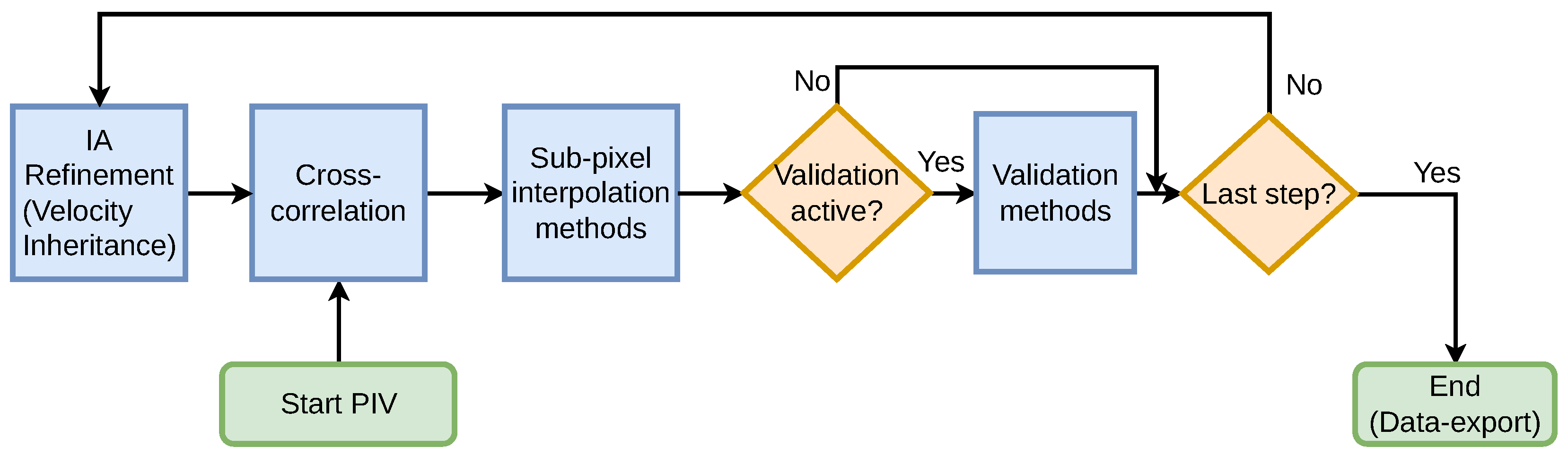
PIV methods typically assume that the region of interest is divided into small areas or volumes (interrogation areas/units—IAs), where the flow is approximately uniform. The motion of a set of particles in the interrogation units is then converted into a velocity vector through cross-correlation and sub-pixel analysis (see
Figure 1). The size of the interrogation units determines the spatial resolution of PIV. Small units improve the resolution but reduce the signal quality, as the method requires several particles in the interrogation unit to obtain a strong correlation peak. Finding the correlation peak with sub-pixel accuracy is fundamental for the overall accuracy of the method. In “adaptive” or “multi-pass” PIV, this workflow is cycled several times, where, at each cycle/step, the interrogation units are refined to smaller sizes, with the number of steps/cycles being predefined by the user. The velocity vectors of each interrogation unit, from the previous step, are inherited by the newly refined units, according to a given inheritance strategy.
The resolution of classic PIV does not increase with the increase in tracer particles in the interrogation units.
Particle Tracking Velocimetry (PTV) can provide a velocity vector per tracer particle [
2,
3], greatly increasing the spatial resolution of classic PIV. The accuracy of Particle Tracking Velocimetry depends on the correct identification of the same particle between consecutive images and on the identification of its centroid with sub-pixel resolution. It is normally not practical for planar (2D) PIV since the out-of-plane loss of particles may reduce its advantages vis-a-vis the added computational cost. It also requires interpolation into regular grids if subsequent analysis requires evenly spaced data.
A different velocimetry technique that may provide denser 2D vector maps is optical flow (OpF). Optical flow estimates the apparent 2D flow resulting from time-varying image brightness intensity through optimization techniques. OpF methods can be classified as gradient-based, e.g., [
4,
5,
6,
7], region-based or feature-based matching [
8,
9,
10], global-matching [
11,
12], spatio-temporal filtering [
13,
14], and, more recently, deep learning methods [
15,
16]. Of the many OpF methods that have been developed since their inception, most of them have specifically targeted machine vision applications; however, fluid mechanics applications started to be explored in the 1990s. The first OpF method for fluid mechanics was probably [
17], featuring a global OpF method and a dynamic programming class algorithm. Other attempts at bringing OpF to the hydraulics and fluid mechanics fields are based on the Horn and Schunck [
4] method. This is the case for [
18] and several variants with different computational constraints [
19,
20,
21,
22]. A few other modern methods developed for fluid mechanics applications include FOLKI [
23,
24], Liu–Shen physics-based OpF [
25], and wOFV [
26,
27]. Theoretically, dense OpF methods can achieve one vector per image pixel. However, the relatively sparse (identifiable) bright dots of PIV images may not allow for such high resolution.
Hybridization is a way to take advantage of favorable image characteristics, such as higher tracer concentrations, or hardware availability, such as several visualization angles by several synchronized cameras, to increase spatial resolution. Few attempts have been made at hybridizing PIV with OpF techniques. The most relevant ones include [
28], with the proposal of a combination of PIV with the OpF method of Liu and Shen [
25], the latter without employing any of the traditional PIV sub-pixel methods. Glomb and Swirniak (2019) [
29] presented methods for hybrid PIV-OpF, as well as hybrid Particle Tracking Velocimetry (PTV), based on PIV and multi-resolution/pyramidal OpF. Seong (2019) [
30] conceived a hybrid PIV-OpF approach with a Horn–Schunck-inspired method [
31] that was adapted to deal with variations in laser intensity for pulsed laser configurations. The works [
32,
33] also developed a hybrid PIV-OpF solution that addresses image intensity variations between successive frames. It uses PIV in connection with Liu–Shen OpF [
25] and with Horn–Schunck [
4] OpF, where the latter provides the initial estimate for the former method. Hybrid methods have the ability to deal with large tracer particle displacements while retrieving dense velocity maps like dense OpF methods. Some hybrid PIV solutions do not require multi-resolution/pyramidal OpF setups to deal with the large displacements, for example, [
28]. The novel hybrid PIV method in [
34] explores a different approach to computing the cross-correlation by considering a circulant matrix and also includes a novel OpF method inspired by the Horn–Schunck formulation that better handles large displacements and that dynamically adjusts its parameters.
In summary, previous PIV-OpF hybridization efforts have attempted to streamline procedures, provide efficient implementations, test novel combinations of methods, or even present novel methods. However, there are many possible hybrid combinations of correlation-based PIV and OpF methods, mostly because there are several available OpF methods. Recently, the study [
35] extensively analyzed various combinations of OpF methods and showed that the combination of the Lucas–Kanade and Liu–Shen OpF methods is the most accurate. To our best knowledge, this combination has not been hybridized with PIV. The first objective of this paper is thus to present a hybrid of correlation-based PIV and a combination of Lucas–Kanade and Liu–Shen OpF methods. We present a novel open-source tool, named QuickLabPIV-ng (
https://github.com/CoreRasurae/QuickLabPIV-ng, accessed on 25 March 2024), that supports hybrid PIV with a combination of the Liu–Shen and Lucas–Kanade OpF methods [
35], where the latter provides the initial estimate for Liu–Shen.
The second objective of this paper is to explore the accuracy of a hybrid PIV method that replaces sub-pixel interpolation with an optical flow (OpF) step to refine the estimation of displacement within each interrogation area. This method aims to address issues related to the size and number of particle images affecting the correlation peak’s shape, which can lead to errors in displacement estimation. By integrating OpF, the process seeks to directly correct the peak location’s integer estimate, potentially circumventing the challenges associated with traditional sub-pixel reconstruction steps in PIV analysis.
Hybrid PIV-OpF methods have been validated against well-known phenomena but not rigorously tested on real turbulent flows critical for environmental studies. Recognizing the importance of denser velocity maps for analyzing turbulence [
36], this paper proposes testing these methods on realistic flows resembling homogeneous isotropic turbulence. Additionally, we highlight the limitations of applying OpF to datasets designed for classic PIV and set out to validate hybrid solutions on real-life turbulent flow data with inherent optical noise, marking a significant step toward practical application.
Finally, we validate the new hybrid PIV method and the sub-pixel OpF-based alternative on synthetic and real laboratory PIV image databases. On the one hand, validation on the synthetic databases is aimed at evaluating the raw accuracy performance by validating the methods against precise ground-truth data, as generated by the PIV image generator tool [
37] (please see
Section 4 for further details about the image generation). On the other hand, validation on real laboratory databases is aimed at evaluating the performance of the methods with respect to turbulent macro- and micro-scale recovery.
This paper is organized as follows. It starts with a review of the proposed PIV software and techniques. It then validates these methods using synthetic images of simple flows as a baseline, assessing errors across various noise levels. The second validation phase applies the software to real experimental data of differing qualities (in terms of image noise, non static background image elements, and varying imaged particle’s sizes and concentrations), including flows around a cylinder, in a rough boundary layer, and plunging flows. The results are analyzed using auto-correlation, structure functions, power spectral density, and dissipation rates. The paper concludes with findings and recommendations for future research.
2. Software Workflow and Main Features
2.1. Workflow and Hybridization Options
We describe the main features and workflow of the hybrid PIV-OpF software, named QuickLabPIV-ng at version v0.8.7. The software is based on the PIV workflow. An initial coarse velocity vector field estimate is obtained by large, user-selected interrogation areas. This initial estimate is based on the cross-correlation of image pairs followed by correlation peak reconstitution to find the location of the peak with sub-pixel accuracy. The initial vector field is then inherited by smaller interrogation areas that may be deformed for better matching. Between the PIV steps, OpF may be used as a substitute for peak reconstruction and peak location. At the end of all the PIV steps, OpF may be used as the last step either to fine-tune the PIV velocity estimate or to provide denser velocity maps. Again, the number of steps/cycles is predefined by the user when selecting the starting and ending IA sizes. Between PIV/OpF steps, a vector inspection may be carried out to validate the flow field. The substitution of wrong vectors may take place. The key aspects of the workflow are depicted in
Figure 2. OpF methods can be either local or global. Local OpF methods operate exclusively with an image region and vectors in the vicinity of the vector under consideration. Global OpF methods depend on the overall image to estimate any single vector and thus cannot operate with small regions.
The software supports three different hybridization variants:
Variant 1—“dense hybrid PIV-OpF”—employs dense optical flow as the last PIV step, either with dense Lucas–Kanade or with dense Liu–Shen combined with Lucas–Kanade. This option will provide densified velocity vector maps with 1 velocity vector per image pixel.
Variant 2—“sub-pixel OpF”—employs optical flow as a substitution for the cross-correlation peak reconstruction and sub-pixel interpolation to find the coordinates of the peak. This is only valid for local optical flow methods like Lucas–Kanade. It directly extracts the sub-pixel movement from the original image by considering the pixels in the vicinity of the center of each IA, thus constituting an alternative to the PIV sub-pixel.
Variant 3—“sparse hybrid PIV-OpF”—is similar to variant 1 but keeps only the velocity vectors of the center of each IA. We refer to this as sparse optical flow (1 velocity vector per each IA), thus keeping the original PIV vector resolution but allowing sub-pixel resolution. This supports both local and global optical flow methods, where a half-pixel warp is performed to obtain velocity pixels aligned with the center of each IA.
The process is iterated until the end of the last adaptive PIV step. Finally, the data are exported in MATLAB file format.
The following sections describe all relevant PIV and OpF methods and algorithms.
2.2. PIV Key Steps—Cross-Correlation and Sub-Pixel Interpolation
QuickLabPIV-ng features IA cross-correlation via a 2D radix-2 FFT as the main PIV method, employing adaptive multi-step processing with customizable IA window sizes. It offers various sub-pixel interpolation methods, including traditional 1D-1D Gaussian three-point polynomial interpolation [
38] and 1D-1D Gaussian robust LR [
39]. Additionally, it supports optical flow methods like Lucas–Kanade and its combination with Liu–Shen; see
Section 2.3.
2.3. OpF Methods
The Lucas–Kanade and Liu–Shen optical flow (OpF) methods enhance fluid mechanics analysis by adapting to a wide range of imaging conditions and particle dynamics (bit depths, particle concentration, spot sizes) [
35]. Lucas–Kanade, a local method, calculates displacement within a defined window, iteratively refining estimates (more details in [
5]). Conversely, Liu–Shen, a global approach, improves the initial velocity estimates by incorporating physical and optical effects of image formation (e.g., light scattering and intensity), requiring a robust starting point from other methods (more details in [
33]). Both techniques necessitate pre-filtering for accuracy and support adaptive iteration counts. While Lucas–Kanade quickly converges, Liu–Shen demands more iterations for refinement. However, Liu–Shen is capable of improving the accuracy over the initial velocity estimations obtained from several other methods [
35]. Additionally, the software accommodates both dense and sparse applications, offering a specialized Liu–Shen mode for clipped images, allowing CPU implementation, albeit with compromised precision.
2.4. Hybridization of OpF and PIV after Correlation Steps
QuickLabPIV-ng enhances PIV analysis by enabling the use of two distinct sub-pixel interpolation methods at various stages, optimizing the initial and final interrogation steps with separate techniques. This dual approach allows for the initial use of either sparse OpF or traditional sub-pixel methods, transitioning to dense OpF methods for final refinement. This strategy not only improves sub-pixel accuracy, particularly in the last steps, but also densifies velocity maps for more detailed results. The software’s flexibility in combining OpF and traditional methods offers significant advantages in precision and computational efficiency, bypassing traditional warping methods for a direct, accurate sub-pixel resolution. While standard sub-pixel techniques determine displacement by analyzing the geometry of cross-correlation peaks, optical flow (OpF) methods directly compute fractional displacement from the raw image. When the interrogation area (IA) size in the final PIV step is smaller than the OpF window, using dense OpF becomes more cost-effective and reduces the drawbacks of global methods. An OpF approach can bypass traditional PIV warping, offering a direct transition to precise sub-pixel measurements, maintaining an accuracy comparable to that of conventional warping techniques.
2.5. Vector Inheritance and Warping
When iterating to the next PIV step, i.e., smaller IA sizes, the processing continues with the refinement of interrogation areas (IAs) into smaller areas and includes a vector inheritance strategy, as well as an IA image warping strategy. When all adaptive PIV steps are completed, PIV processing proceeds with a possible hybridization (either variant 1 or variant 3). If hybridization is to be performed, then a single pass of optical flow is applied. We refer to methods featuring image warping as “Modern PIV”.
2.5.1. Vector Inheritance
The vector inheritance strategy involves selecting a method—area, distance, or bi-cubic spline interpolation—to import velocity vectors before adjusting the second image’s interrogation area (IA) windows accordingly for cross-correlation. Each method offers a unique way to calculate new IA displacements based on previous steps: area inheritance uses a weighted average from overlapping IA areas (see
Figure 2), distance inheritance applies weights inversely proportional to the center distances of adjacent IAs, and bi-cubic spline inheritance interpolates displacements using a 2D map of IA centers. The Bi-cubic spline is noted for its superior accuracy in validations with synthetic image databases (see
Section 3).
2.5.2. IA Image Warping
Window warping PIV employs backward image warping or a blend of window displacement and image warping, rather than shifting interrogation areas (IAs) by inherited displacements. This approach includes full or partial warping methods—traditional warping, mini-warping, and micro-warping. Traditional warping applies bi-cubic spline-interpolated displacements to each pixel, ensuring no voids or overlaps and maintaining fixed IA window locations. Mini-warping and micro-warping adjust IA windows based on estimated displacements, with micro-warping focusing on integer displacements followed by fractional warping for precision. QuickLabPIV-ng supports various configurations for applying warping to enhance PIV accuracy, with micro-warping on the second image showing the best results in validations; see
Section 3.
2.6. Vector Validation and Substitution
Vector validation in PIV systems identifies and addresses incorrect velocity vectors caused by a low SNR, insufficient correlatable data, or other issues like boundary effects and particle movement. QuickLabPIV-ng offers methods to mark invalid vectors as zero or “not a number” for data export and to correct for such vectors where feasible, using a combination of validation and vector replacement techniques. These techniques ensure the reliability of the velocity data by effectively identifying and addressing outliers.
QuickLabPIV-ng implements two primary methods for vector validation: difference validation and normalized median validation [
38]. The first evaluates the differences in the velocity vector within a local grid, flagging those that exceed a set threshold as invalid. The latter uses a median-based approach, comparing each vector with the median vector within its vicinity against a normalized threshold to determine validity.
where
denotes the vector with the median Euclidean norm of all the vectors in the neighbor IAs;
is the vector under analysis;
is the median of the residuals
, where
indexes the neighbor IAs; and
is a regularization term between
and
pixels.
QuickLabPIV-ng offers two methods for vector replacement: bi-linear and multi-peak. Bi-linear interpolation generates a new vector from valid neighboring vectors, while multi-peak searches for alternative high-correlation peaks as potential replacements, assuming the primary peak might be noise-distorted. If multi-peak fails, it defaults to bi-linear interpolation. The software also supports iterative validation to refine vector accuracy, though with caution to avoid misjudging valid vectors as invalid. This process enhances data reliability, especially in low-signal-to-noise scenarios.
4. Methods and Materials
We cannot provide the test databases online due to their sheer size, as we would not be able to guarantee the medium- to long-term availability of the contents. We thus prefer to provide instructions to generate similar ones for the synthetic image database. As for the experimental databases, the authors are willing to provide them upon request.
It should, however, be noted that these databases are not a critical part of the article and that their role is just to document the PIV and hybrid PIV methods’ capabilities. As such, the results presented are expected to be compatible with other results obtained from other databases with similar characteristics.
Other than that, as of this writing, the recommended version to reproduce these results is QuickLabPIV-ng v0.8.7, obtainable from
https://github.com/CoreRasurae/QuickLabPIV-ng/releases/tag/v0.8.7 (accessed on 25 March 2024). The software itself does most of the computation without requiring external libraries/frameworks; namely, image filtering, cross-correlation, and Lucas–Kanade and Liu–Shen optical flow methods are implemented internally, which should protect the software from bit-rot, as well as unexpected behavioral changes coming from external library updates. Even with this effort made, it was not completely possible to avoid an important dependency on the Aparapi (
https://aparapi.com (accessed on 25 March 2024),
https://git.cleverthis.com/cleverthis/aparapi/aparapi/-/releases/v3.0.2 (accessed on 25 March 2024)) library/framework, which enables High-Performance Computing (HPC) for Java in systems with GPU or CPU devices supporting OpenCL.
Besides the software, it requires a computer with at least 32 to 64 GB of RAM for medium- to large-sized databases. Ideally, the system should be a multi-core computer with at least one AMD® or NVIDIA® GPU. Discrete Intel® GPUs have not been tested yet, but integrated Intel® GPUs are known to produce invalid results with the current versions of QuickLabPIV-ng/Aparapi. A Java virtual machine compatible with at least Java 8 should be employed, and it has been tested in both Windows® and Linux environments. Currently, QuickLabPIV-ng only supports image depths of 8 bits from the GUI. We ran our databases on a system with 64GB of RAM by invoking QuickLabPIV-ng with java -Xmx48G -jar QuickLabPIVng.jar.
displayFlowField=false;
closeFlowField=true;
flows={′uniform′ ′parabolic′ ′stagnation′ ...;
′rankine_vortex′ ′rk_uniform′};
bitDepths=[8];
deltaXFactor=[0.05 0.10 0.25];
particleRadius=[0.5 1.0 1.5 3.0];
Ni=[1 6 12 16];
noiseLevel=[0 5 15];
outOfPlaneStdDeviation=[0.025 0.050 0.100];
numberOfRuns=10;
generatePIVImagesWithAllParametersCombinations;
All software was developed in-house and is available as open-source. The PIV hardware equipment, namely the PIV Laser lighting and image acquisition hardware, was obtained from Dantec Dynamics A/S, Skovlunde, Denmark.
5. Conclusions and Recommendations for Further Analysis
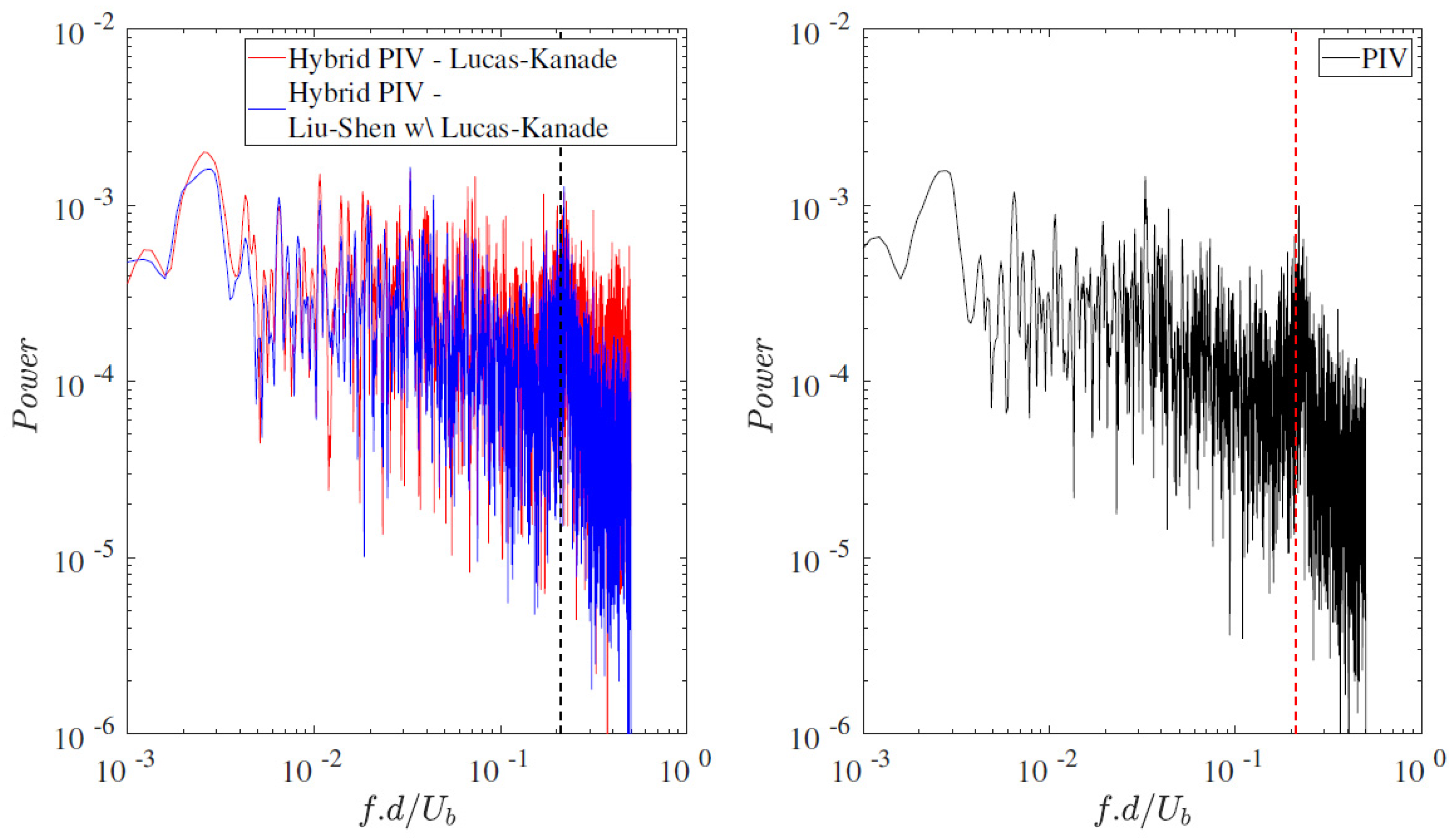
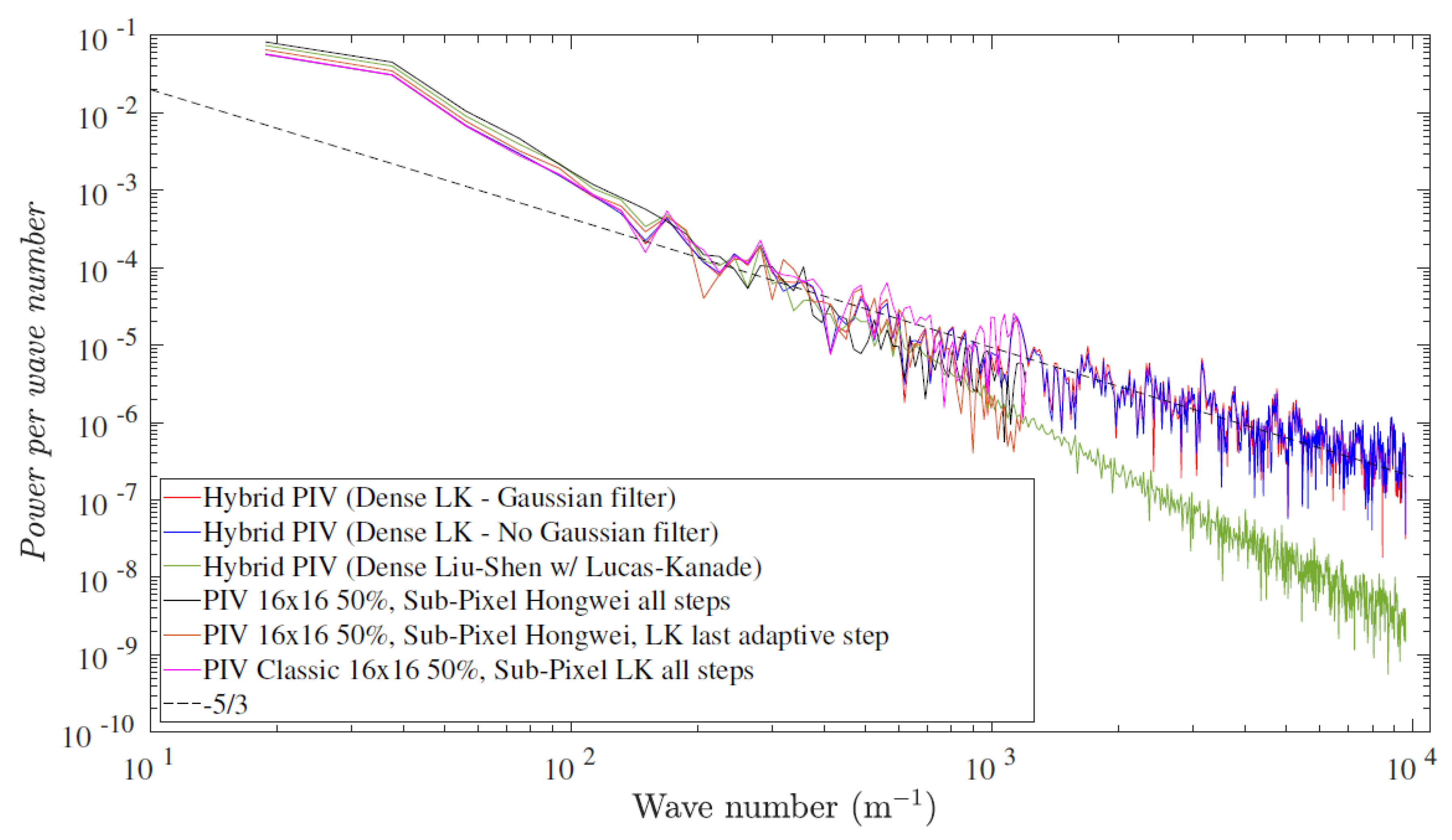
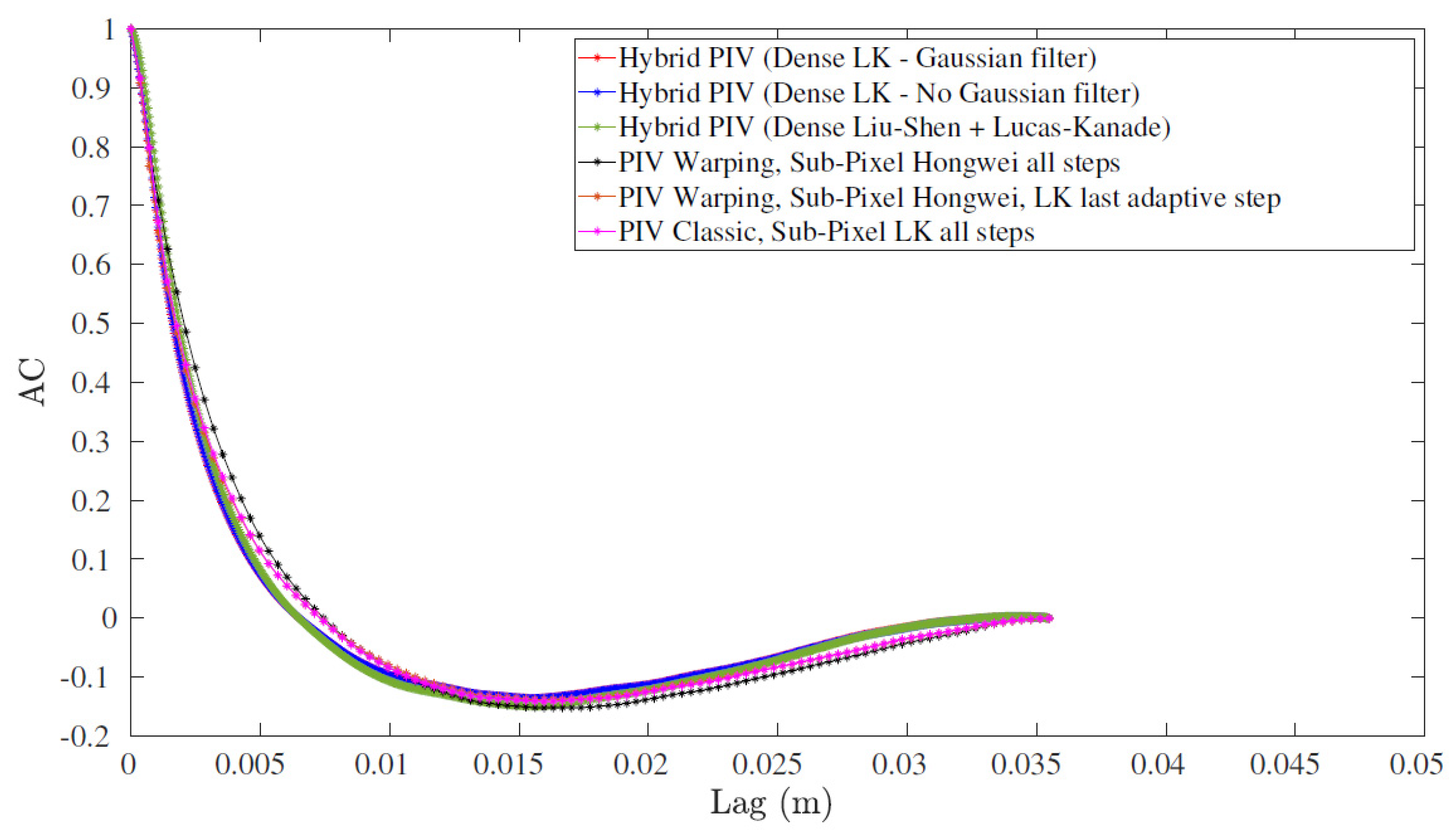
The main conclusion of this research is that hybrid PIV-OpF can improve PIV’s resolution and ability to provide data adequate to analyze fine-scale turbulence. While a better resolution of the mean flow is easy to achieve, turbulence statistics are improved only if the raw PIV images are of good quality, i.e., are within the optical range of tracer density and spot size, and have low optical noise. Hybrid PIV with Liu–Shen and Lucas–Kanade offers the highest accuracy in the description of the mean flow. However, in real databases, it may not closely follow the expected PSD slope of −5/3, despite extending the slope for higher frequencies, suggesting a potential for noise filtering.
To analyze turbulence, the Lucas–Kanade algorithm alone is preferable. It correctly reproduces the flow’s macro-scales and the slope of the power spectral density function and does so in locally isotropic homogeneous turbulence. It is also computationally more efficient.
Integrating Liu–Shen with Lucas–Kanade optical flow (OpF) as an alternative to interpolation peak reconstitution with sub-pixel accuracy is a valid alternative, especially in essentially 2D flows with high-quality images. In this case, the method achieves the accuracy of traditional PIV methods employing warping. PIV’s last adaptive step with a Lucas–Kanade OpF step maintains the standard PIV workflow while leveraging the precision benefits of optical flow techniques.
From our experience, independently of the method, the optimal image conditions include particle sizes around 3 px and at least 6 particles per IA, improving with higher concentrations. For the analysis of PIV sequences, a tailored approach is recommended for optimal results. For classic PIV incorporating optical flow (OpF) for sub-pixel refinement, the sparse Lucas–Kanade method is preferred. If initial sub-pixel interpolation deviates significantly from expectations, it is advisable to limit the OpF application to the final refinement stage. For advanced PIV techniques, including window warping, a combination of Hongwei Guo’s robust Gaussian regression and dense Lucas–Kanade with Liu-Shen OpF, adjusted for the last adaptive step, enhances accuracy. The Lagrange multiplier in the Liu–Shen method is sensitive to the pixel’s brightness range, so it is recommended to normalize the pixel intensities to a fixed range, which QuickLabPIV-ng does automatically. For validation with vector substitution, it is recommended to use a normalized median combined with multi-peak replacement with four peaks around the main peak and a search kernel set with a width of 3 pixels. These strategies, validated through synthetic imagery, align with the evolving needs of PIV analysis, ensuring precise and reliable measurements under various experimental conditions.
Our preliminary examination across the three PIV image databases with real experimental data suggests promising potential for hybrid PIV techniques, particularly when integrating Lucas–Kanade methods, in broadening the scope of turbulence measurements achievable with PIV. However, this exploration is just the beginning. More comprehensive studies are imperative to fully harness and understand the capabilities and limitations of these advanced methodologies. Additionally, the impact of Gaussian filtering on the fidelity of Taylor micro-scale readings warrants further investigation, as it could inadvertently obscure crucial data.


 ,
, 


