
Response of Floods to the Underlying Surface Changes in the Taojiang River Basin Using the Hydrologic Engineering Center’s Hydrologic Modeling System
Abstract
:1. Introduction
2. Study and Data
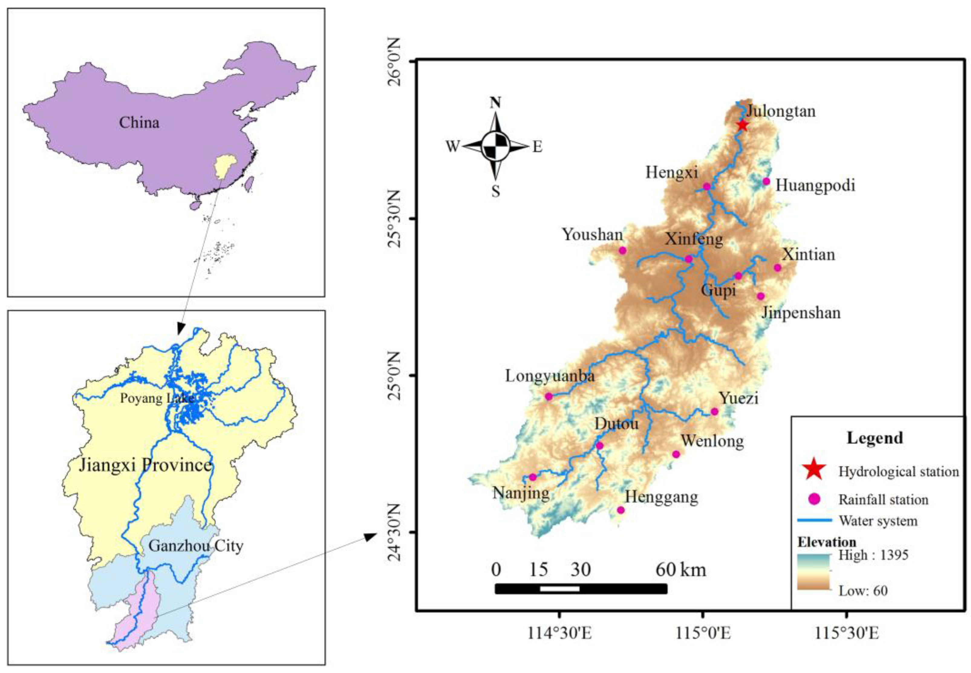
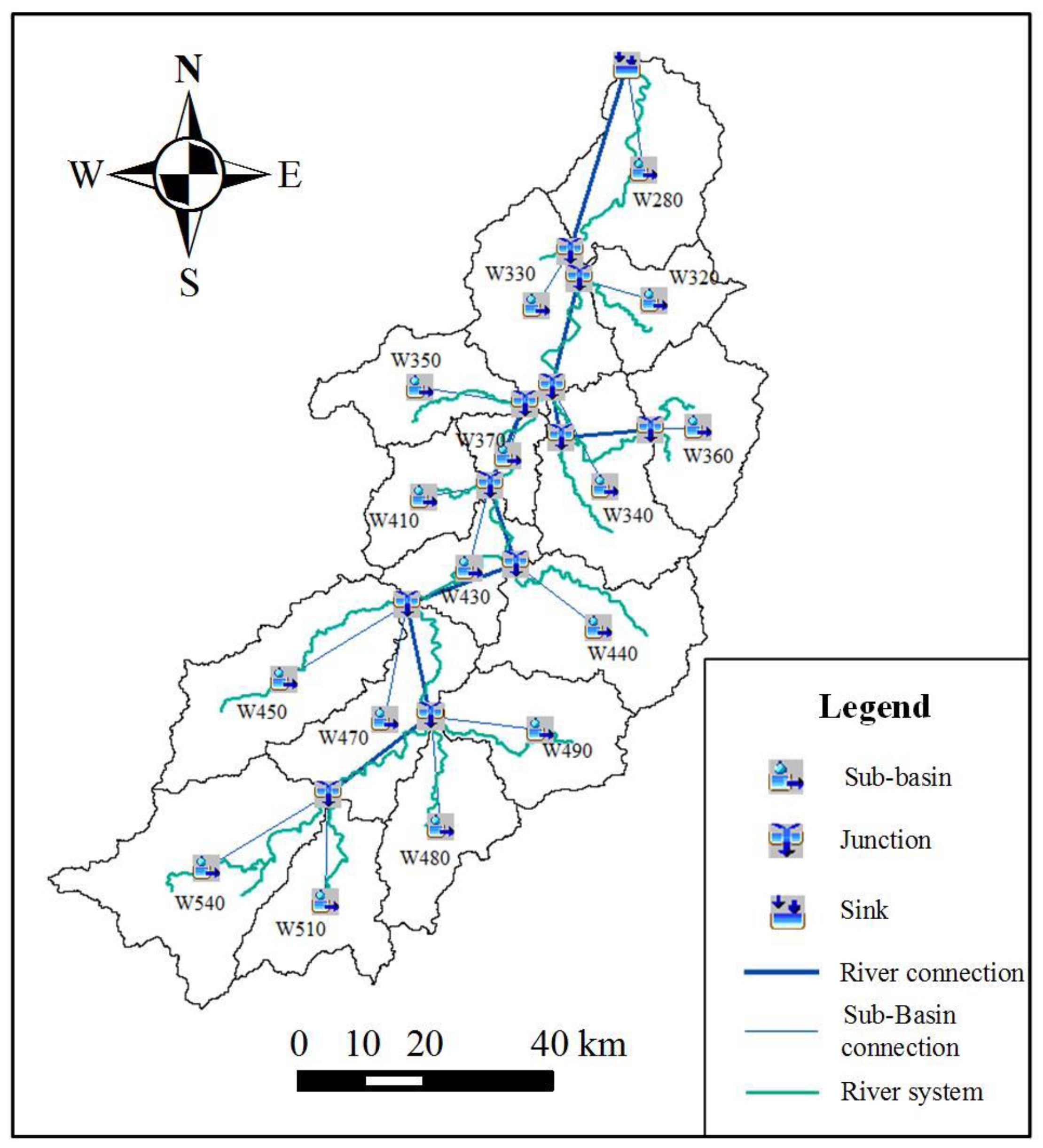
2.1. Study Area
2.2. Data
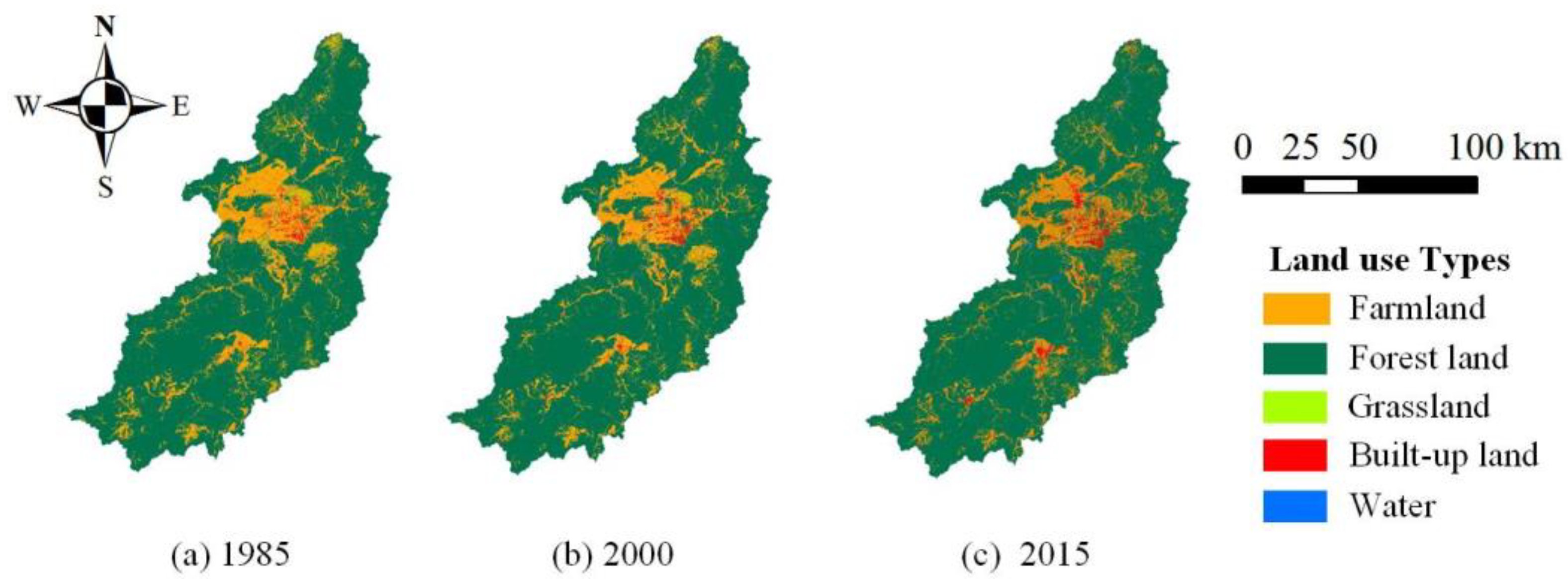
3. Characteristic Analysis of the USCs
4. Methods
4.1. HEC-HMS Model
4.1.1. Loss Model
4.1.2. Transform Model
4.1.3. Base Flow Model
4.1.4. Routing Model
4.2. Model Evaluation
4.3. Flood Simulation Methods for Various Underlying Surface Scenarios
5. Results and Analysis
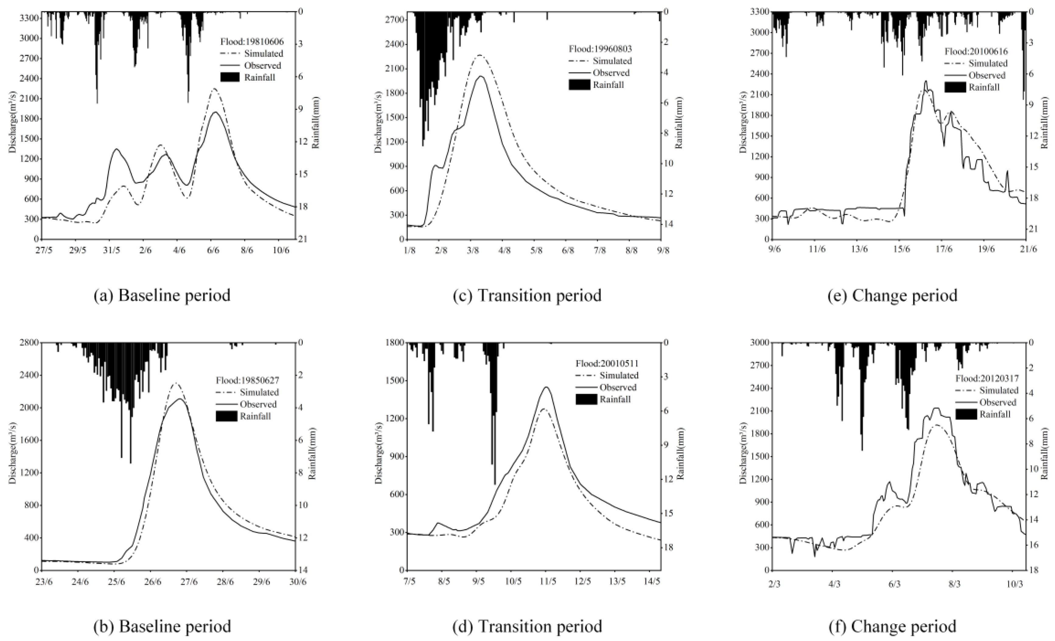
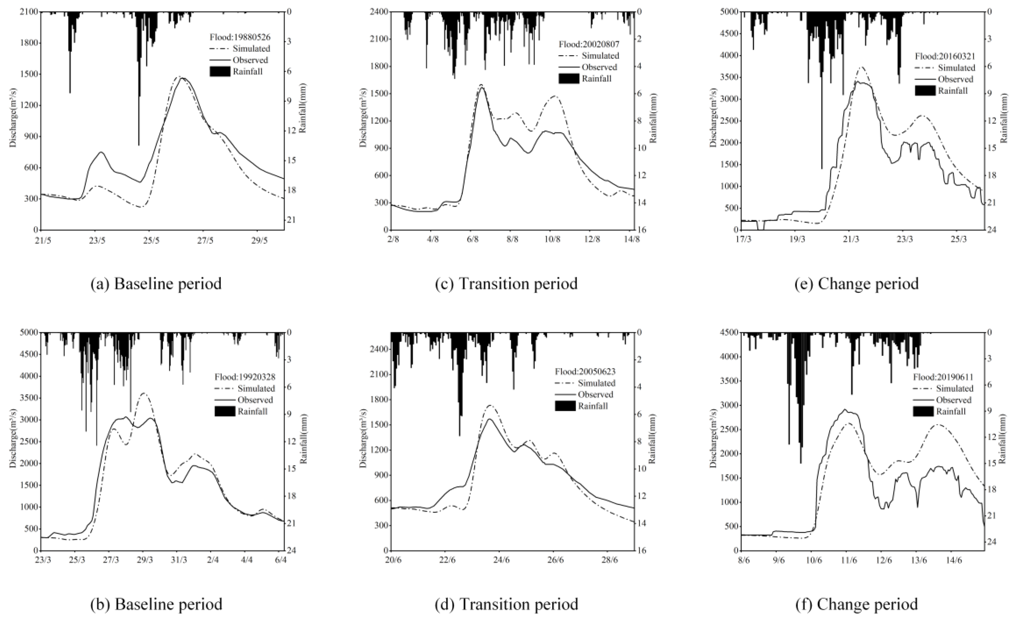
5.1. Evaluation and Analysis of Flood Simulation
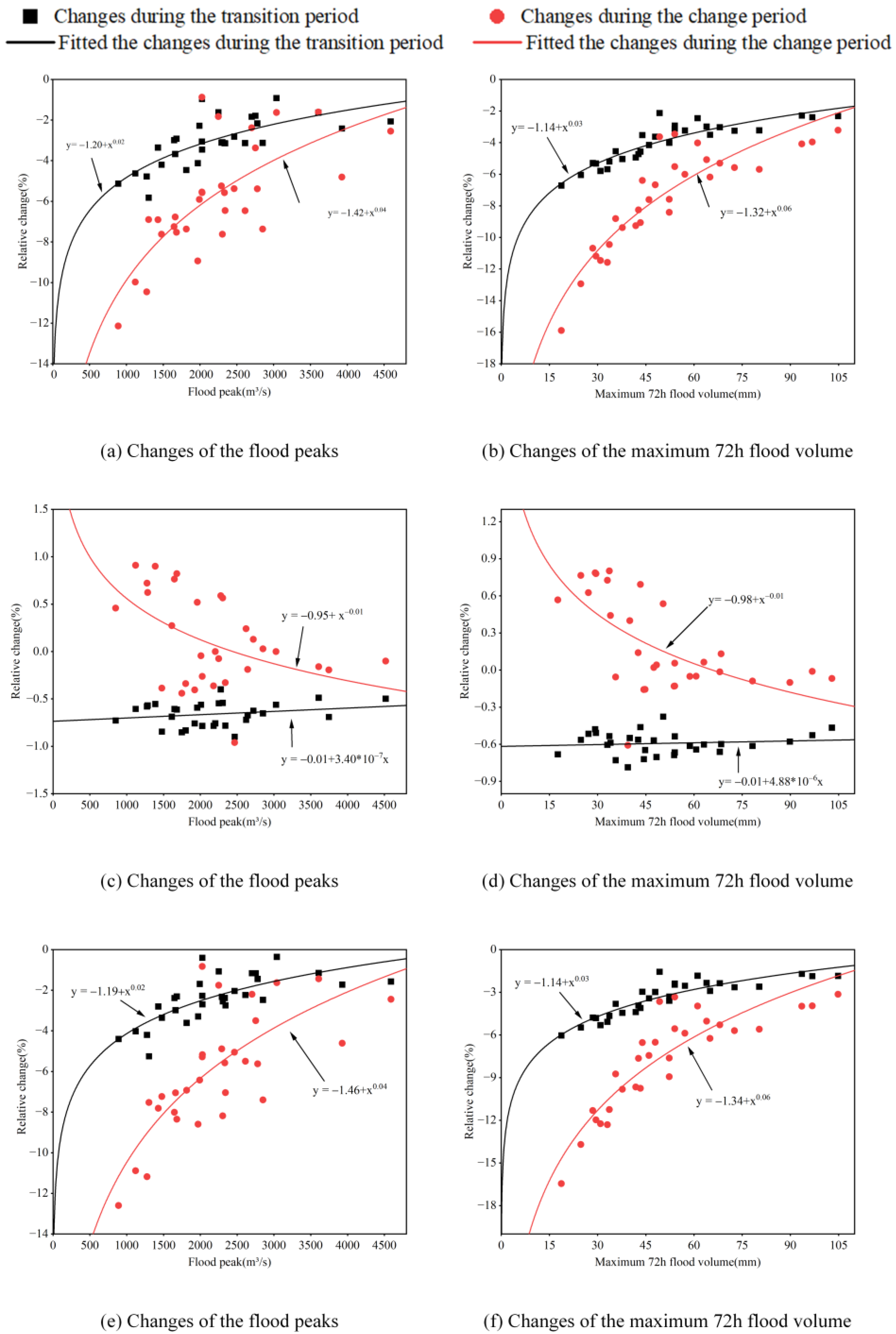
5.2. Response of Floods to USCs
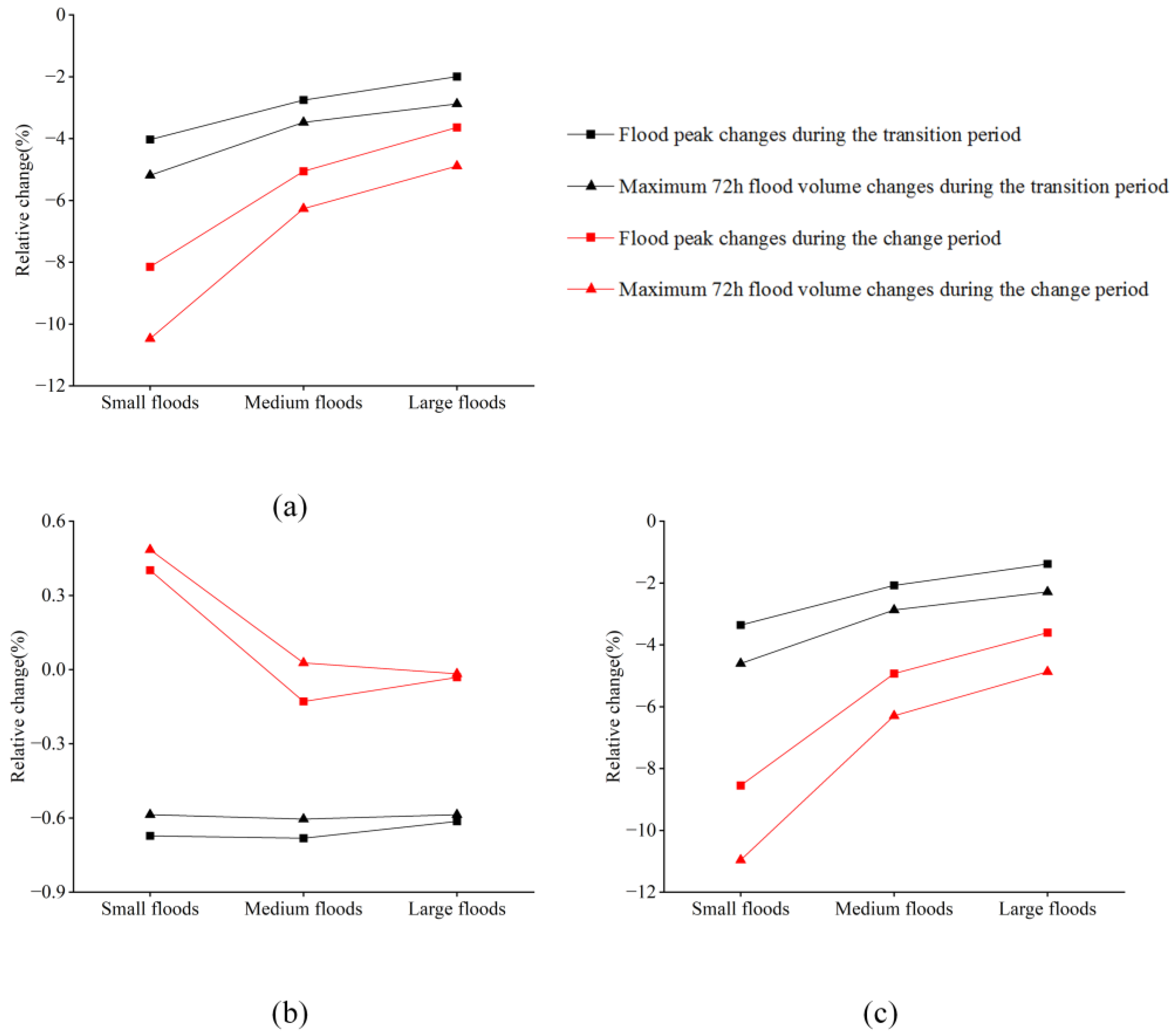
5.3. Analysis of the Response of Floods of Different Magnitudes to USCs
6. Conclusions
Author Contributions
Funding
Data Availability Statement
Conflicts of Interest
Appendix A

| Flood Number | Flood Peak (m3/s) | Maximum 72 h Flood Volume (mm) | ||||||||
|---|---|---|---|---|---|---|---|---|---|---|
| Baseline Period | Transition Period | Relative Change (%) | Change Period | Relative Change (%) | Baseline Period | Transition Period | Relative Change (%) | Change Period | Relative Change (%) | |
| 19810606 | 2250.4 | 2213.9 | −1.62 | 2209.2 | −1.83 | 54.03 | 52.45 | −2.92 | 52.16 | −3.46 |
| 19840428 | 1276 | 1215 | −4.78 | 1142.5 | −10.46 | 29.49 | 27.92 | −5.32 | 26.19 | −11.19 |
| 19850627 | 2304.9 | 2233.6 | −3.09 | 2129.3 | −7.62 | 43.34 | 41.36 | −4.57 | 39.41 | −9.07 |
| 19850925 | 1681.2 | 1632.1 | −2.92 | 1554.6 | −7.53 | 33.06 | 31.18 | −5.69 | 29.23 | −11.58 |
| 19860606 | 2026.5 | 1964.5 | −3.06 | 1914.1 | −5.55 | 54.01 | 52.32 | −3.13 | 51.03 | −5.52 |
| 19940621 | 4590 | 4495 | −2.07 | 4472.9 | −2.55 | 104.87 | 102.44 | −2.32 | 101.5 | −3.21 |
| 19950618 | 2753 | 2703.7 | −1.79 | 2660.1 | −3.37 | 65.02 | 62.74 | −3.51 | 61 | −6.18 |
| 19960803 | 2342.7 | 2269 | −3.15 | 2191.4 | −6.46 | 52.31 | 50.23 | −3.98 | 47.91 | −8.41 |
| 19980310 | 3039.3 | 3011.3 | −0.92 | 2989.7 | −1.63 | 80.32 | 77.73 | −3.22 | 75.75 | −5.69 |
| 20010511 | 1303.5 | 1227.6 | −5.82 | 1213.5 | −6.90 | 28.53 | 27.02 | −5.29 | 25.48 | −10.69 |
| 20080614 | 2333.5 | 2260.2 | −3.14 | 2203.4 | −5.58 | 52.34 | 50.24 | −4.01 | 48.37 | −7.59 |
| 20090704 | 2612.2 | 2530.3 | −3.14 | 2443.4 | −6.46 | 42.72 | 40.7 | −4.73 | 39.19 | −8.26 |
| 20100616 | 2292.6 | 2221.3 | −3.11 | 2172.3 | −5.25 | 61.14 | 59.64 | −2.45 | 58.68 | −4.02 |
| 20110517 | 2702.5 | 2652.8 | −1.84 | 2638 | −2.39 | 63.93 | 62.02 | −2.99 | 60.68 | −5.08 |
| 20120317 | 2028.8 | 1958.7 | −3.46 | 1915.6 | −5.58 | 47.94 | 46.2 | −3.63 | 44.74 | −6.68 |
| Flood Number | Flood Peak (m3/s) | Maximum 72 h Flood Volume (mm) | ||||||||
|---|---|---|---|---|---|---|---|---|---|---|
| Baseline Period | Transition Period | Relative Change (%) | Change Period | Relative Change (%) | Baseline Period | Transition Period | Relative Change (%) | Change Period | Relative Change (%) | |
| 19810606 | 2250.4 | 2238.1 | −0.55 | 2248.7 | −0.08 | 54.03 | 53.74 | −0.54 | 53.96 | −0.13 |
| 19840428 | 1276 | 1268.6 | −0.58 | 1285.2 | 0.72 | 29.49 | 29.34 | −0.51 | 29.72 | 0.78 |
| 19850627 | 2304.9 | 2292.4 | −0.54 | 2317.9 | 0.56 | 43.34 | 43.14 | −0.46 | 43.64 | 0.69 |
| 19850925 | 1681.2 | 1670.9 | −0.61 | 1695 | 0.82 | 33.06 | 32.86 | −0.60 | 33.3 | 0.73 |
| 19860606 | 2026.5 | 2010.6 | −0.78 | 2021.2 | −0.26 | 54.01 | 53.65 | −0.67 | 54.04 | 0.06 |
| 19940621 | 4517.5 | 4495 | −0.50 | 4512.9 | −0.10 | 102.92 | 102.44 | −0.47 | 102.85 | −0.07 |
| 19950618 | 2720.7 | 2703.7 | −0.62 | 2724.2 | 0.13 | 63.12 | 62.74 | −0.60 | 63.16 | 0.06 |
| 19960803 | 2278.1 | 2269 | −0.40 | 2291.5 | 0.59 | 50.42 | 50.23 | −0.38 | 50.69 | 0.54 |
| 19980310 | 3028.3 | 3011.3 | −0.56 | 3028.3 | 0.00 | 78.21 | 77.73 | −0.61 | 78.14 | −0.09 |
| 20010511 | 1284.9 | 1277.6 | −0.57 | 1292.9 | 0.62 | 27.16 | 27.02 | −0.52 | 27.33 | 0.63 |
| 20080614 | 2203.7 | 2187 | −0.76 | 2203.7 | 0.00% | 48.35 | 48.01 | −0.70 | 48.37 | 0.04 |
| 20090704 | 2467.1 | 2444.9 | −0.90 | 2443.4 | −0.96% | 39.43 | 39.12 | −0.79 | 39.19 | −0.61 |
| 20100616 | 2180.2 | 2163.1 | −0.78 | 2172.3 | −0.36% | 58.71 | 58.35 | −0.61 | 58.68 | −0.05 |
| 20110517 | 2643 | 2625.2 | −0.67 | 2638 | −0.19% | 60.71 | 60.32 | −0.64 | 60.68 | −0.05 |
| 20120317 | 1923.4 | 1908.8 | −0.76 | 1915.6 | −0.41% | 44.81 | 44.52 | −0.65 | 44.74 | −0.16 |
| Flood Types | USCs | LUCs | SWCMs | |||||||||
|---|---|---|---|---|---|---|---|---|---|---|---|---|
| Relative Change in Flood Peak (%) | Relative Change in Maximum 72 h Flood Volume (%) | Relative Change in Flood Peak (%) | Relative change in Maximum 72 h Flood Volume (%) | Relative Change in Flood Peak (%) | Relative Change in Maximum 72 h Flood Volume (%) | |||||||
| Transition Period | Change Period | Transition Period | Change Period | Transition Period | Change Period | Transition Period | Change Period | Transition Period | Change Period | Transition Period | Change Period | |
| Small flood | −4.03 | −8.15 | −5.19 | −10.47 | −0.67 | 0.40 | 0.59 | 0.49 | −3.36 | −8.55 | −4.60 | −10.96 |
| Medium flood | −2.75 | −5.06 | −3.48 | −6.27 | −0.68 | −0.13 | −0.60 | 0.03 | −2.07 | −4.93 | −2.87 | −6.29 |
| Large flood | −2.00 | −3.64 | −2.87 | −4.89 | −0.61 | −0.03 | −0.59 | −0.02 | −1.38 | −3.61 | −2.29 | −4.87 |
References
- Yang, D.; Yang, Y.; Xia, J. Hydrological Cycle and Water Resources in a Changing World: A Review. Geogr. Sustain. 2021, 2, 115–122. [Google Scholar] [CrossRef]
- Prokešová, R.; Horáčková, Š.; Snopková, Z. Surface Runoff Response to Long-Term Land Use Changes: Spatial Rearrangement of Runoff-Generating Areas Reveals a Shift in Flash Flood Drivers. Sci. Total Environ. 2022, 815, 151591. [Google Scholar] [CrossRef] [PubMed]
- Feng, B.; Zhang, Y.; Bourke, R. Urbanization Impacts on Flood Risks Based on Urban Growth Data and Coupled Flood Models. Nat. Hazards 2021, 106, 613–627. [Google Scholar] [CrossRef]
- Le Floch, N.; Pons, V.; Hassan Abdalla, E.M.; Alfredsen, K. Catchment Scale Effects of Low Impact Development Implementation Scenarios at Different Urbanization Densities. J. Hydrol. 2022, 612, 128178. [Google Scholar] [CrossRef]
- Zhao, Y.; Xia, J.; Xu, Z.; Qiao, Y.; Shen, J.; Ye, C. Impact of Urbanization on Regional Rainfall-Runoff Processes: Case Study in Jinan City, China. Remote Sens. 2023, 15, 2383. [Google Scholar] [CrossRef]
- Guoyi, L.; Liu, J.; Shao, W. Urban Flood Risk Assessment under Rapid Urbanization in Zhengzhou City, China. Reg. Sustain. 2023, 4, 332–348. [Google Scholar] [CrossRef]
- Janizadeh, S.; Chandra Pal, S.; Saha, A.; Chowdhuri, I.; Ahmadi, K.; Mirzaei, S.; Mosavi, A.H.; Tiefenbacher, J.P. Mapping the Spatial and Temporal Variability of Flood Hazard Affected by Climate and Land-Use Changes in the Future. J. Environ. Manag. 2021, 298, 113551. [Google Scholar] [CrossRef] [PubMed]
- Xiao, L.; Robinson, M.; O’Connor, M. Woodland’s Role in Natural Flood Management: Evidence from Catchment Studies in Britain and Ireland. Sci. Total Environ. 2022, 813, 151877. [Google Scholar] [CrossRef]
- Luo, J.; Zhou, X.; Rubinato, M.; Li, G.; Tian, Y.; Zhou, J. Impact of Multiple Vegetation Covers on Surface Runoff and Sediment Yield in the Small Basin of Nverzhai, Hunan Province, China. Forests 2020, 11, 329. [Google Scholar] [CrossRef]
- Ghalehteimouri, K.J.; Ros, F.C.; Rambat, S. Flood Risk Assessment through Rapid Urbanization LULC Change with Destruction of Urban Green Infrastructures Based on NASA Landsat Time Series Data: A Case of Study Kuala Lumpur between 1990–2021. Acta Ecol Sin. 2023, in press. [Google Scholar] [CrossRef]
- Gabriels, K.; Willems, P.; Van Orshoven, J. A Comparative Flood Damage and Risk Impact Assessment of Land Use Changes. Nat. Hazards Earth Syst. Sci. 2022, 22, 395–410. [Google Scholar] [CrossRef]
- Liu, Y.; Han, J.; Jiao, J.; Liu, B.; Ge, W.; Pan, Q.; Wang, F. Responses of Flood Peaks to Land Use and Landscape Patterns under Extreme Rainstorms in Small Catchments—A Case Study of the Rainstorm of Typhoon Lekima in Shandong, China. Int. Soil Water Conserv. Res. 2022, 10, 228–239. [Google Scholar] [CrossRef]
- Du, X.; Jian, J.; Du, C.; Stewart, R.D. Conservation Management Decreases Surface Runoff and Soil Erosion. Int. Soil Water Conserv. Res. 2022, 10, 188–196. [Google Scholar] [CrossRef]
- Yaekob, T.; Tamene, L.; Gebrehiwot, S.G.; Demissie, S.S.; Adimassu, Z.; Woldearegay, K.; Mekonnen, K.; Amede, T.; Abera, W.; Recha, J.W.; et al. Assessing the Impacts of Different Land Uses and Soil and Water Conservation Interventions on Runoff and Sediment Yield at Different Scales in the Central Highlands of Ethiopia. Renew. Agric. Food Syst. 2022, 37, S73–S87. [Google Scholar] [CrossRef]
- Liu, Y.; Han, J.; Liu, Y.; Zhang, S.; Min, L.; Liu, B.; Jiao, J.; Zhang, L. Effects of Soil and Water Conservation Measures of Slope Surfaces on Flood Peaks of Small Watersheds: A Study Based on Three Extreme Rainstorm Events in Northern China. CATENA 2023, 232, 107432. [Google Scholar] [CrossRef]
- Zhao, Y.; Cao, W.; Hu, C.; Wang, Y.; Wang, Z.; Zhang, X.; Zhu, B.; Cheng, C.; Yin, X.; Liu, B.; et al. Analysis of Changes in Characteristics of Flood and Sediment Yield in Typical Basins of the Yellow River under Extreme Rainfall Events. CATENA 2019, 177, 31–40. [Google Scholar] [CrossRef]
- Fu, S.; Yang, Y.; Liu, B.; Liu, H.; Liu, J.; Liu, L.; Li, P. Peak Flow Rate Response to Vegetation and Terraces under Extreme Rainstorms. Agric. Ecosyst. Environ. 2020, 288, 106714. [Google Scholar] [CrossRef]
- Zhu, T.X. Effectiveness of Conservation Measures in Reducing Runoff and Soil Loss Under Different Magnitude–Frequency Storms at Plot and Catchment Scales in the Semi-Arid Agricultural Landscape. Environ. Manag. 2016, 57, 671–682. [Google Scholar] [CrossRef]
- Yuan, F.; Yang, G.; Zhang, Q.; Li, H. Soil Erosion Assessment of the Poyang Lake Basin, China: Using USLE, GIS and Remote Sensing. J. Remote Sens. GIS 2016, 5, 12. [Google Scholar] [CrossRef]
- Li, X.; Hu, Q.; Zhang, Q.; Wang, R. Response of Rainfall Erosivity to Changes in Extreme Precipitation in the Poyang Lake Basin, China. J. Soil Water Conserv. 2020, 75, 537–548. [Google Scholar] [CrossRef]
- Wen, T.; Xiong, L.; Jiang, C.; Xu, X.; Liu, Z. Attribution analysis of annual sediment load of Ganjiang River Basin using BMA based on time-varying moment models. Trans. Chin. Soc. Agric. Eng. 2021, 37, 140–149. (In Chinese) [Google Scholar]
- Keller, A.A.; Garner, K.; Rao, N.; Knipping, E.; Thomas, J. Hydrological Models for Climate-Based Assessments at the Watershed Scale: A Critical Review of Existing Hydrologic and Water Quality Models. Sci. Total Environ. 2023, 867, 161209. [Google Scholar] [CrossRef] [PubMed]
- Hamdan, A.N.A.; Almuktar, S.; Scholz, M. Rainfall-Runoff Modeling Using the HEC-HMS Model for the Al-Adhaim River Catchment, Northern Iraq. Hydrology 2021, 8, 58. [Google Scholar] [CrossRef]
- Guduru, J.U.; Jilo, N.B.; Rabba, Z.A.; Namara, W.G. Rainfall-Runoff Modeling Using HEC-HMS Model for Meki River Watershed, Rift Valley Basin, Ethiopia. J. Afr. Earth Sci. 2023, 197, 104743. [Google Scholar] [CrossRef]
- Azam, M.; Kim, H.S.; Maeng, S.J. Development of Flood Alert Application in Mushim Stream Watershed Korea. Int. J. Disaster Risk Reduct. 2017, 21, 11–26. [Google Scholar] [CrossRef]
- Lin, Q.; Lin, B.; Zhang, D.; Wu, J. Web-Based Prototype System for Flood Simulation and Forecasting Based on the HEC-HMS Model. Environ. Model. Softw. 2022, 158, 105541. [Google Scholar] [CrossRef]
- Tu, H.; Wang, X.; Zhang, W.; Peng, H.; Ke, Q.; Chen, X. Flash Flood Early Warning Coupled with Hydrological Simulation and the Rising Rate of the Flood Stage in a Mountainous Small Watershed in Sichuan Province, China. Water 2020, 12, 255. [Google Scholar] [CrossRef]
- Patel, P.; Thakur, P.K.; Aggarwal, S.P.; Garg, V.; Dhote, P.R.; Nikam, B.R.; Swain, S.; Al-Ansari, N. Revisiting 2013 Uttarakhand Flash Floods through Hydrological Evaluation of Precipitation Data Sources and Morphometric Prioritization. Geomat. Nat. Hazards Risk 2022, 13, 646–666. [Google Scholar] [CrossRef]
- Davtalab, R.; Mirchi, A.; Khatami, S.; Gyawali, R.; Massah, A.; Farajzadeh, M.; Madani, K. Improving Continuous Hydrologic Modeling of Data-Poor River Basins Using Hydrologic Engineering Center’s Hydrologic Modeling System: Case Study of Karkheh River Basin. J. Hydrol. Eng. 2017, 22, 05017011. [Google Scholar] [CrossRef]
- Ben Khélifa, W.; Mosbahi, M. Modeling of Rainfall-Runoff Process Using HEC-HMS Model for an Urban Ungauged Watershed in Tunisia. Model. Earth Syst. Environ. 2022, 8, 1749–1758. [Google Scholar] [CrossRef]
- Younis, S.M.Z.; Ammar, A. Quantification of Impact of Changes in Land Use-Land Cover on Hydrology in the Upper Indus Basin, Pakistan. Egypt. J. Remote Sens. Space Sci. 2018, 21, 255–263. [Google Scholar] [CrossRef]
- Yan, X.; Lin, M.; Chen, X.; Yao, H.; Liu, C.; Lin, B. A New Method to Restore the Impact of Land-use Change on Flood Frequency Based on the Hydrologic Engineering Center-Hydrologic Modelling System Model. Land Degrad. Dev. 2020, 31, 1520–1532. [Google Scholar] [CrossRef]
- Gao, Y.; Chen, J.; Luo, H.; Wang, H. Prediction of Hydrological Responses to Land Use Change. Sci. Total Environ. 2020, 708, 134998. [Google Scholar] [CrossRef] [PubMed]
- Kabeja, C.; Li, R.; Guo, J.; Rwatangabo, D.E.R.; Manyifika, M.; Gao, Z.; Wang, Y.; Zhang, Y. Erratum: Kabeja, C.; et al. The Impact of Reforestation Induced Land Cover Change (1990–2017) on Flood Peak Discharge Using HEC-HMS Hydrological Model and Satellite Observations: A Study in Two Mountain Basins, China. Water 2021, 13, 676, Erratum in Water 2020, 12, 1347. [Google Scholar] [CrossRef]
- Zhao, S.; Luo, P.; Liu, H. Spatial-temporal variation characteristics of different grades of rainfall in Taojiang River Basin along upper reaches of Ganjiang River. J. Nanchang Inst. Technol. 2022, 41, 32–39. (In Chinese) [Google Scholar]
- Şengül, S.; İspirli, M.N. Predicting Snowmelt Runoff at the Source of the Mountainous Euphrates River Basin in Turkey for Water Supply and Flood Control Issues Using HEC-HMS Modeling. Water 2022, 14, 284. [Google Scholar] [CrossRef]
- Rammal, M.; Berthier, E. Runoff Losses on Urban Surfaces during Frequent Rainfall Events: A Review of Observations and Modeling Attempts. Water 2020, 12, 2777. [Google Scholar] [CrossRef]
- Gao, B.; Xu, Y.; Sun, Y.; Wang, Q.; Wang, Y.; Li, Z. The Impacts of Impervious Surface Expansion and the Operation of Polders on Flooding under Rapid Urbanization Processes. Theor. Appl. Climatol. 2023, 151, 1215–1225. [Google Scholar] [CrossRef]
- Halwatura, D.; Najim, M.M.M. Application of the HEC-HMS Model for Runoff Simulation in a Tropical Catchment. Environ. Model. Softw. 2013, 46, 155–162. [Google Scholar] [CrossRef]
- Tassew, B.G.; Belete, M.A.; Miegel, K. Application of HEC-HMS Model for Flow Simulation in the Lake Tana Basin: The Case of Gilgel Abay Catchment, Upper Blue Nile Basin, Ethiopia. Hydrology 2019, 6, 21. [Google Scholar] [CrossRef]
- GB/T22482-2008; Standard for Hydrological Information and Hydrological Forecasting. CHINESE GB Standards: Beijing, China, 2008. (In Chinese)
- Yao, C.; Chang, L.; Ding, J.; Li, Z.; An, D.; Zhang, Y. Evaluation of the Effects of Underlying Surface Change on Catchment Hydrological Response Using the HEC-HMS Model. Proc. Int. Assoc. Hydrol. Sci. 2014, 364, 145–150. [Google Scholar] [CrossRef]
- Lehbab-Boukezzi, Z.; Boukezzi, L.; Errih, M. Uncertainty Analysis of HEC-HMS Model Using the GLUE Method for Flash Flood Forecasting of Mekerra Watershed, Algeria. Arab. J. Geosci. 2016, 9, 751. [Google Scholar] [CrossRef]
- Natarajan, S.; Radhakrishnan, N. Simulation of Rainfall–Runoff Process for an Ungauged Catchment Using an Event-Based Hydrologic Model: A Case Study of Koraiyar Basin in Tiruchirappalli City, India. J. Earth. Syst. Sci. 2021, 130, 30. [Google Scholar] [CrossRef]
- Glas, R.; Hecht, J.; Simonson, A.; Gazoorian, C.; Schubert, C. Adjusting Design Floods for Urbanization across Groundwater-Dominated Watersheds of Long Island, NY. J. Hydrol. 2023, 618, 129194. [Google Scholar] [CrossRef]
- Wei, L.; Hu, K.; Hu, X. Rainfall Occurrence and Its Relation to Flood Damage in China from 2000 to 2015. J. Mt. Sci. 2018, 15, 2492–2504. [Google Scholar] [CrossRef]


| Land-Use Types | 1985 | 2000 | 2015 | |||
|---|---|---|---|---|---|---|
| Area (km2) | Proportion (%) | Area (km2) | Proportion (%) | Area (km2) | Proportion (%) | |
| Farmland | 1367.87 | 17.39 | 1216.39 | 15.47 | 1208.16 | 15.36 |
| Forest land | 6312.65 | 80.27 | 6470.33 | 82.28 | 6447.18 | 81.98 |
| Grassland | 45.95 | 0.58 | 17.42 | 0.22 | 5.39 | 0.07 |
| Built-up land | 101.54 | 1.29 | 121.09 | 1.54 | 161.19 | 2.05 |
| Water | 36.00 | 0.46 | 38.78 | 0.49 | 42.08 | 0.54 |
| Total | 7864.00 | 100 | 7864.00 | 100 | 7864.00 | 100 |
| Land-Use Types | Soil Hydrological Groups | |||
|---|---|---|---|---|
| A | B | C | D | |
| Farmland | 65 | 75 | 82 | 86 |
| Forest land | 25 | 55 | 70 | 77 |
| Grassland | 30 | 58 | 71 | 78 |
| Built-up land | 69 | 80 | 86 | 90 |
| Water | 92 | 92 | 92 | 92 |
| Sub-Basin Number | CN of Sub-Basin | Imperviousness of Sub-Basin (%) | ||||
|---|---|---|---|---|---|---|
| 1985 | 2000 | 2015 | 1985 | 2000 | 2015 | |
| W490 | 57.66 | 57.74 | 58.71 | 0.29 | 0.57 | 1.49 |
| W480 | 59.20 | 58.48 | 59.85 | 0.63 | 1.04 | 2.69 |
| W470 | 57.74 | 57.47 | 57.64 | 0.71 | 0.82 | 0.93 |
| W450 | 56.45 | 56.14 | 56.41 | 0.10 | 0.13 | 0.19 |
| W440 | 57.29 | 57.25 | 57.71 | 0.27 | 0.39 | 0.96 |
| W430 | 60.62 | 59.77 | 59.57 | 0.76 | 0.99 | 1.32 |
| W410 | 66.41 | 65.01 | 64.31 | 2.48 | 2.87 | 3.26 |
| W370 | 73.00 | 71.39 | 70.57 | 11.40 | 13.13 | 14.84 |
| W360 | 56.78 | 56.72 | 57.01 | 0.28 | 0.32 | 0.49 |
| W350 | 66.50 | 65.4 | 64.79 | 2.04 | 2.75 | 3.75 |
| W340 | 64.31 | 63.72 | 62.92 | 6.62 | 7.31 | 7.64 |
| W330 | 61.37 | 60.98 | 60.86 | 1.02 | 1.23 | 2.22 |
| W320 | 57.71 | 58.06 | 58.08 | 0.29 | 0.41 | 0.60 |
| W540 | 57.87 | 57.38 | 57.64 | 0.40 | 0.50 | 0.98 |
| W510 | 57.07 | 56.94 | 56.97 | 0.19 | 0.27 | 0.41 |
| W280 | 57.48 | 57.25 | 57.3 | 0.32 | 0.34 | 0.48 |
| Accuracy Level | A | B | C |
|---|---|---|---|
| QR (%) | QR ≥ 85 | 85 > QR ≥ 70 | 70 > QR ≥ 60 |
| DC | DC > 0.9 | 0.9 ≥ DC ≥ 0.7 | 0.7 > DC ≥ 0.5 |
| Scenario Name | Scenario Settings | Participation during Simulated Flood Events |
|---|---|---|
| S1 | Soil erosion conditions in 1985 + land-use conditions in 1985 | All thirty events |
| S2 | Soil erosion conditions in 1985 + land-use conditions in 2000 | Ten events during the baseline period |
| S3 | Soil erosion conditions in 1985 + land-use conditions in 2015 | Ten events during the baseline period |
| S4 | Soil erosion conditions in 2000 + land-use conditions in 1985 | Ten events during the transition period |
| S5 | Soil erosion conditions in 2000 + land-use conditions in 2000 | All thirty events |
| S6 | Soil erosion conditions in 2000 + land-use conditions in 2015 | Ten events during the transition period |
| S7 | Soil erosion conditions in 2015 + land-use conditions in 1985 | Ten events during the change period |
| S8 | Soil erosion conditions in 2015 + land-use conditions in 2000 | Ten events during the change period |
| S9 | Soil erosion conditions in 2015 + land-use conditions in 2015 | All thirty events |
| Simulation Periods | Flood Number | REP (%) | REV (%) | Δt (h) | DC | Qualified (Q)/ Failed (F) | |
|---|---|---|---|---|---|---|---|
| Baseline period | Calibration | 19810606 | 18.44 | −9.89 | −1 | 0.71 | Q |
| 19840428 | −12.60 | −15.05 | 1 | 0.91 | Q | ||
| 19850627 | 9.24 | 2.98 | −2 | 0.97 | Q | ||
| 19850925 | 3.14 | 13.06 | −1 | 0.94 | Q | ||
| 19860606 | 8.95 | 8.87 | −2 | 0.79 | Q | ||
| 19870517 | −26.68 | −19.18 | 1 | 0.84 | F | ||
| Verification | 19880526 | 1.27 | −16.19 | −1 | 0.84 | Q | |
| 19890523 | −16.38 | −13.36 | −2 | 0.93 | Q | ||
| 19900412 | −15.45 | −13.97 | −1 | 0.89 | Q | ||
| 19920328 | 17.53 | 0.02 | 26 | 0.92 | F | ||
| Transition period | Calibration | 19940621 | 28.06 | 8.81 | −8 | 0.90 | F |
| 19950618 | −0.96 | 6.81 | −8 | 0.93 | F | ||
| 19960803 | 12.89 | 12.42 | 0 | 0.79 | Q | ||
| 19980310 | 4.56 | −5.32 | −2 | 0.82 | Q | ||
| 20010511 | −11.89 | −15.68 | −1 | 0.88 | Q | ||
| 20020807 | 2.04 | 9.87 | −1 | 0.80 | Q | ||
| Verification | 20030519 | −5.95 | −10.27 | −5 | 0.90 | F | |
| 20040408 | 8.18 | 14.71 | −1 | 0.85 | Q | ||
| 20050623 | 10.42 | −3.73 | 1 | 0.85 | Q | ||
| 20060523 | −12.56 | −15.09 | 0 | 0.85 | Q | ||
| Change period | Calibration | 20080614 | −5.84 | 6.50 | 1 | 0.90 | Q |
| 20090704 | 13.65 | 12.69 | 5 | 0.92 | F | ||
| 20100616 | −5.55 | 2.44 | −2 | 0.90 | Q | ||
| 20110517 | 14.70 | 9.56 | 3 | 0.92 | Q | ||
| 20120317 | −10.49 | −10.20 | 1 | 0.90 | Q | ||
| 20150521 | −1.37 | 5.12 | 5 | 0.82 | F | ||
| Verification | 20160321 | 9.67 | 9.18 | 3 | 0.84 | Q | |
| 20190310 | 8.04 | 2.12 | 2 | 0.61 | Q | ||
| 20190611 | −9.96 | 16.29 | 3 | 0.60 | Q | ||
| 20200404 | 6.52 | 15.83 | 6 | 0.78 | F | ||
| Simulation Periods | Average Flood Peak (m3/s) | Average Maximum 72 h Flood Volume (mm) | Relative Change in Flood Peak (%) | Relative Change in Maximum 72 h Flood Volume (%) |
|---|---|---|---|---|
| Baseline period | 2240 | 52.13 | - | - |
| Transition period | 2178 | 50.27 | −3.06 | −4.00 |
| Change period | 2122 | 48.72 | −5.92 | −7.58 |
| Simulation Periods | LUCs | SWCMs | ||||
|---|---|---|---|---|---|---|
| Average Flood Peak (m3/s) | Average Maximum 72 h Flood Volume (mm) | Relative Change in Flood Peak (%) | Relative Change in Maximum 72 h Flood Volume (%) | Relative Change in Flood Peak (%) | Relative Change in Maximum 72 h Flood Volume (%) | |
| Baseline period | 2186 | 50.48 | - | - | - | - |
| Transition period | 2172 | 50.18 | −0.66 | −0.59 | −2.40 | −3.41 |
| Change period | 2187 | 50.54 | 0.11 | 0.20 | −6.03 | −7.78 |
Disclaimer/Publisher’s Note: The statements, opinions and data contained in all publications are solely those of the individual author(s) and contributor(s) and not of MDPI and/or the editor(s). MDPI and/or the editor(s) disclaim responsibility for any injury to people or property resulting from any ideas, methods, instructions or products referred to in the content. |
© 2024 by the authors. Licensee MDPI, Basel, Switzerland. This article is an open access article distributed under the terms and conditions of the Creative Commons Attribution (CC BY) license (https://creativecommons.org/licenses/by/4.0/).
Share and Cite
Xiao, Y.; Wen, T.; Gu, P.; Xiong, B.; Xu, F.; Chen, J.; Zou, J. Response of Floods to the Underlying Surface Changes in the Taojiang River Basin Using the Hydrologic Engineering Center’s Hydrologic Modeling System. Water 2024, 16, 1120. https://doi.org/10.3390/w16081120
Xiao Y, Wen T, Gu P, Xiong B, Xu F, Chen J, Zou J. Response of Floods to the Underlying Surface Changes in the Taojiang River Basin Using the Hydrologic Engineering Center’s Hydrologic Modeling System. Water. 2024; 16(8):1120. https://doi.org/10.3390/w16081120
Chicago/Turabian StyleXiao, Yong, Tianfu Wen, Ping Gu, Bin Xiong, Fei Xu, Junlin Chen, and Jiayu Zou. 2024. "Response of Floods to the Underlying Surface Changes in the Taojiang River Basin Using the Hydrologic Engineering Center’s Hydrologic Modeling System" Water 16, no. 8: 1120. https://doi.org/10.3390/w16081120