Article

A Research on Multi-Index Intelligent Integrated Prediction Model of Catchment Pollutant Load under Data Scarcity

State Key Laboratory of Water Resources Engineering and Management, Wuhan University, Wuhan 430072, China
*
Authors to whom correspondence should be addressed.
Water 2024, 16(8), 1132; https://doi.org/10.3390/w16081132
Submission received: 25 March 2024 / Revised: 14 April 2024 / Accepted: 15 April 2024 / Published: 16 April 2024

Abstract

:
Within a river catchment, the relationship between pollutant load migration and its related factors is nonlinear generally. When neural network models are used to identify the nonlinear relationship, data scarcity and random weight initialization might result in overfitting and instability. In this paper, we propose an averaged weight initialization neural network (AWINN) to realize the multi-index integrated prediction of a pollutant load under data scarcity. The results show that (1) compared with the particle swarm optimization neural network (PSONN) and AdaboostR models that prevent overfitting, AWINN improved simulation accuracy significantly. The R2 in test sets of different pollutant load models reached 0.51–0.80. (2) AWINN is effective in overcoming instability. With more hidden layers, the stability of the models’ outputs was stronger. (3) Sobol sensitivity analysis explained that the main influencing factors of the whole process were the flows of the catchment inlet and outlet, and main factors changed across seasons. The algorithm proposed in this paper can realize stably integrated prediction of pollutant load in the catchment under data scarcity and help to understand the mechanism that influences pollutant load migration.

1. Introduction

Water pollution caused by human activities has become a vital element that affects the health of rivers and is an obstacle to sustainable development [1]. The change in water quality is related to water quality upstream, migration of pollutants from the catchment, and hydrodynamic factors [2,3]. The pollutant load from a catchment is the first reason that brings uncertainty to the corresponding water environment. Because of the influences of nature and human activities, the inner mechanism of pollutant load generation, migration, and reduction has the characteristics of high dimension and complex nonlinearity [4]. The synthesis simulation of the nonlinear relationship between pollutant loads and factors within a catchment has become a hotpot in the field of water pollution control [5].
The methods of pollutant load simulation include the coefficient model, statistical model, process-based model, and machine learning model. The export coefficient model (ECM) builds the relationship between pollutant loads and pollution sources by coefficients to predict pollutant loads [6]. To avoid the uncertainty from precipitation and terrain, researchers developed the improved export coefficient model (IECM) [7]. Nevertheless, coefficient models make it hard to consider the integrated effects of multiple factors. Statistics models (e.g., multiple linear regression (MLR)) were considered to simulate pollutant loads, but the statistical method did not yield a good generalization [8]. With the in-depth study of non-point source pollution, more process-based models such as SWAT and AGNPS have been widely used in simulating pollutant loads [9,10]. Process-based models need many practical measured variables and model parameters, and they are not fit in regions that lack data. The models mentioned above make it hard to reach a trade-off between model precision and data accessibility. So, there are limitations in researching water pollutant loads systematically.
Machine learning models are always seen as black boxes that can link various input data and output data. Until now, machine learning has become an important means of realizing the integrated simulation of different types of water pollution. Machine learning studies related to water pollution have been involved in the following aspects: (1) recognizing the relationships between the targeted water-quality indicator and other water-quality indicators that are monitored easily by investigating the special relationships of water-quality indicators in different positions [3,11,12,13], (2) predicting time series of water-quality indicators [14,15,16,17], (3) simulating water-quality indicators by remote sensing information [18,19], and (4) extending some influencing factors into the input of machine learning models. Some unknown influences from river channels, natural conditions, and human activities have been considered in simulations [20,21,22,23,24]. However, integrated simulations of water pollutant loads that include socioeconomic data have rarely been considered in machine learning models.
Usually, machine learning models’ generalization ability is weak under data scarcity [25]. As the most widely used machine learning model, the neural network (NN) model also faces the problem of overfitting when data are deficient. The model’s structure and the random initialization of weight are two main reasons [26]. To overcome the problem of overfitting in NN models, many methods have been proposed, such as (1) dropout and L-regularization methods, which randomly reduce neurons and increase the penalty term of the loss function during the training process to avoid the model falling into local optimum [27]; (2) ensemble learning methods, which integrate multiple models to reduce overfitting caused by a single model [28]; (3) data dimension reduction methods like principal component analysis (PCA) that can select the most relevant factors and reduce the influences of redundant factors on model training [29]; (4) intelligent training methods like particle swarm optimization (PSO), the genetic algorithm (GA), or the cuckoo algorithm (CA) that can search the global optimum effectively in the training process [30,31,32,33]; (5) deep learning structures like RNN or CNN that can understand the deep structures of data by changing the structures of neural network models [14,34,35]; and (6) other machine learning methods, like support vector machine (SVM), the adaptive neural fuzzy inference system (ANFIS), and extreme learning machine (ELM), which are based on theories such as hyperplane and fuzzy inference to improve generalization ability [3,12,36]. These methods address the overfitting problem to some extent; however, methods that fully mine available poor data to improve generalization ability are lacking research.
Stability refers to the property of a model being able to maintain a certain range of output when the model is disturbed. In addition to overfitting, it is also an important feature for measuring the generalization ability of machine learning models. Stable machine learning models can generate reliable results [37]. Under data scarcity, random weight initialization will make neural network models over-fitted and unstable. There are two types of initialization methods, including non-pre-training initialization and pre-training initialization [38]. Non-pre-training initialization methods can improve the overfitting problem partly by adjusting the initial weight to adapt to the model structure [38,39,40]. Pre-training initialization methods extract the information from the trained NN model weights to determine the final initial weights [41]. Go et al. (2004) clustered the weights in the weight space and took the average of the cluster centers as the initial weights to classify vegetation types corresponding to the spectral data and achieved good classification results [42]. However, it needs to be verified whether the accuracy and stability of the NN model using the pre-training initialization method can be improved when fitting the regressive relationship of variables under data scarcity.
In addition to stable and accurate machine learning simulation of water pollutant loads, the identification of the main influencing factors in water pollutant load migration is helpful to understanding the inner mechanism of water pollution [43]. However, the black-box nature of NN models makes them difficult to interpret. Up to now, some researches have employed local sensitivity analysis to explain the importance of factors, and they have neglected the mutual influence of factors [44]. Some machine learning models, like random forest (RF), have an interpretable mechanism inside [45]. But they are hardly used to identify the main factors in the case of multi-index. As a global sensitivity analysis method, Sobol sensitivity analysis could overcome the shortcomings mentioned above [46].
The goal of this study is to improve the stability and accuracy of neural network models in the integrated prediction of multi-index pollutant loads under data scarcity. The proposed averaged weight initialization neural network (AWINN) model can solve this problem well. The Sobol sensitivity analysis method is used to identify the temporal variation of influencing factors globally. The remainder of the paper is organized as follows. In Section 2, the study area background and the methods applied in the study are introduced. Accuracy and stability comparisons of different methods and sensitivity analyses are displayed in Section 3. The effects of different factors on AWINN model outputs and the variations in different seasons can be seen in Section 4. Finally, Section 5 introduces the main conclusions.

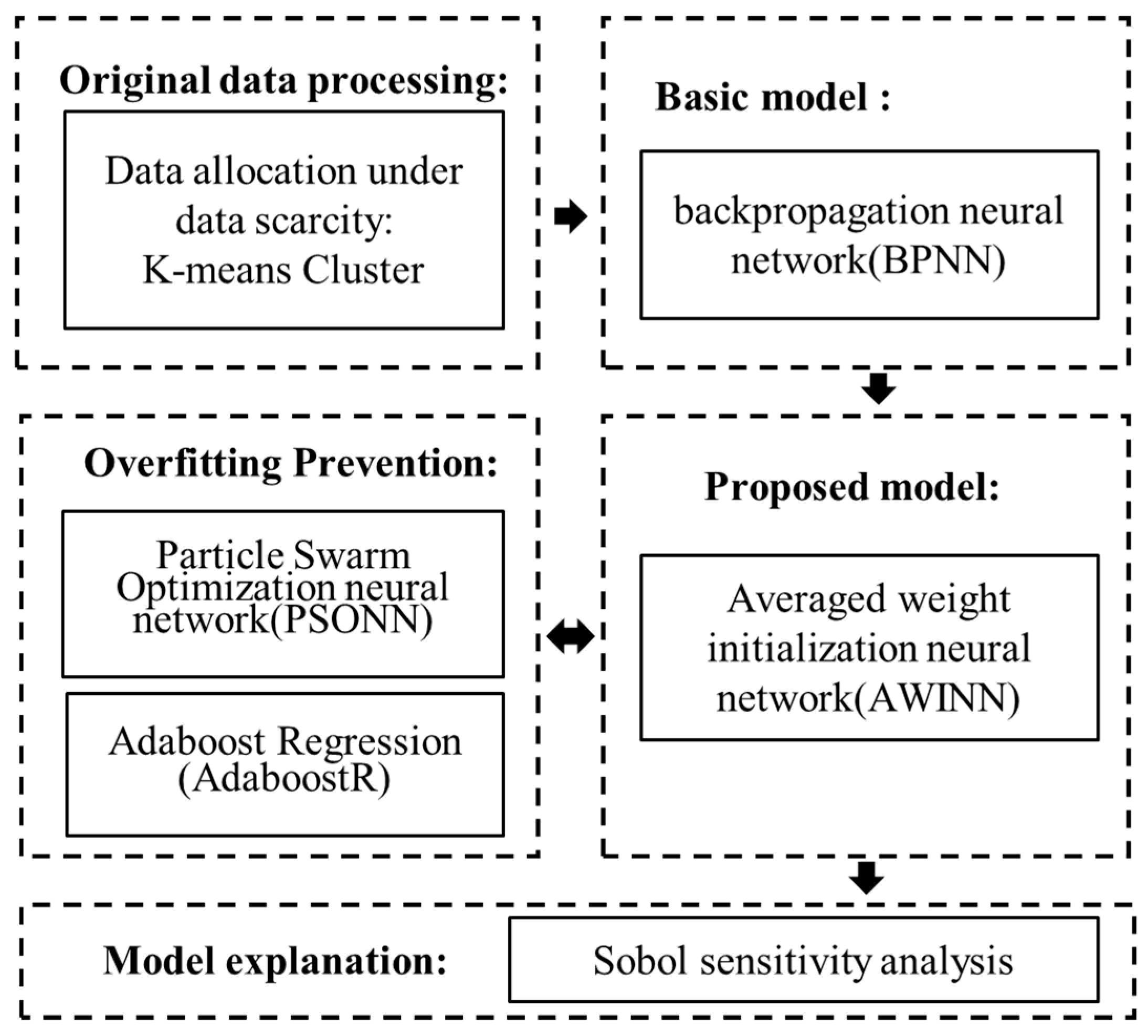
2. Materials and Methods
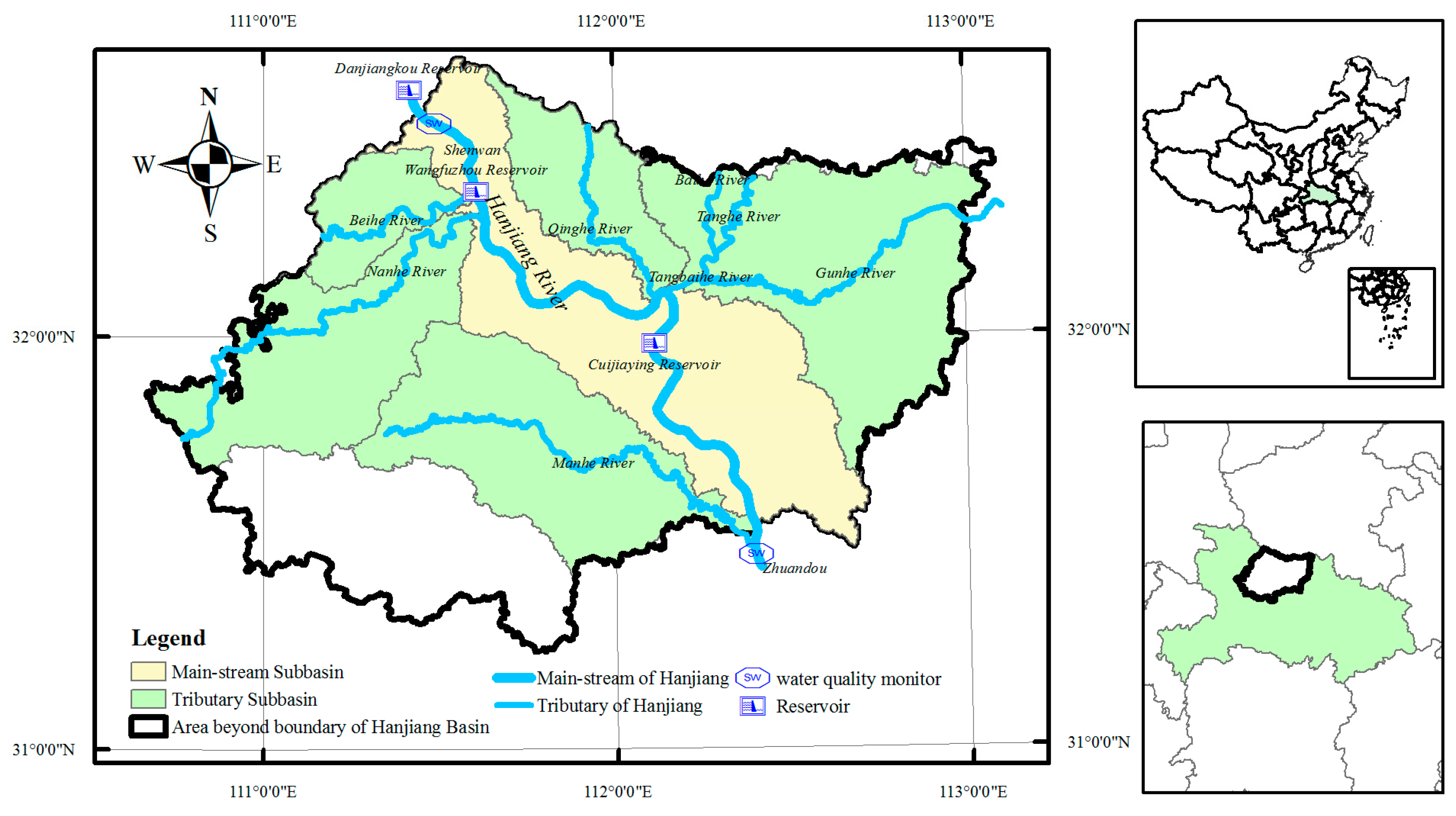
2.1. Study Area

The Xiangyang section of the Hanjiang River catchment lies between 31 ° 13 32 ° 38 N and 110 ° 45 113 ° 7   E , and occupies most of the area of Xiangyang City in Hubei province, China (Figure 1). Mean annual precipitation is 904.45 mm, with the precipitation from May to October accounting for 79.2% of the annual precipitation. The main reach of the Hanjiang River flows from northwest to southeast of Xiangyang City, and many tributaries (the Tangbaihe River, the Nanhe River, the Qinghe River, etc.) flow into the main reach, which transports all pollutant loads of the catchment. Upstream of the study area, Danjiangkou Reservoir is the water source of the middle line of the south-to-north water transfer project, the largest water transfer project in the world. Meanwhile, the catchment is about to take on the water from the Water Diversion Project from Three Gorges Reservoir to the Hanjiang River. The water environment of this catchment is of great significance to the healthy development of the middle and lower reaches of the Hanjiang River.
According to new statistical data, the population of the river catchment is 5.68 million, and urban residents account for 35.1% of the population. The annual disposable income per urban resident is CNY 37,300, and the number is increasing year by year. Agricultural and sideline food processing, automobile manufacturing, the textile industry, and non-metallic mineral product, chemical raw material, and chemical product manufacturing are the main sectors of Xiangyang City’s industry. Urban wastewater treatment capacity has reached 0.337 billion tons per year, and the rate of wastewater treatment is 92.3%. Winter wheat, rice, and corn are the main crop types, and plant areas include 0.355, 0.202, and 0.198 million hectares, respectively. The area of farmland accounts for 36.98% of the whole city, to which around 35.6 tons of chemical fertilizer are applied every year, the highest in Hubei province. Irrigation and precipitation drive pollutant loads from farmland into rivers. Livestock and poultry production accounts for 13.66% of Hubei province. It could be concluded that the region’s pollutant migration is affected by multiple sources and factors.

2.2. Data Collection

Monthly data on pollutant-associated influencing factors in the Xiangyang region from 2015 to 2017 were adopted. The related factors in the input dataset of the study were collected in categories, as shown in Table 1. Different from previous studies, which ignored the socio-economic factors, this study extensively considered the impact of socio-economic factors from towns to villages. The data sources are shown in Table 2. The details of the data processing of the collected data can be seen in Appendix A. Variables with monthly monitoring data are identified by *.
The output data had the problem of uneven distribution, and the monthly pollution load values were concentrated in 5000–20,000 t/mon (88.9%, COD (chemical oxygen demand)), 0–6000 t/mon (91.7%, NH4-N (ammonia nitrogen)), and 0–200 t/mon (69.4%, TP (total phosphorus)). The calculation and distribution of the output data can be seen in Appendix B.

2.3. Methodology

This study executed an NN model training with a backpropagation neural network (BPNN) algorithm. The model fitted to the dataset in the study by a BPNN with random weight initialization had the problems of overfitting and instability. The accuracy of the test set fluctuated greatly after the training set and validation set of the BPNN models reached the standard. It can be concluded that the models were overfitted. When the accuracy of the BPNN models with random weight initialization in the training, validation, and test sets was met, the sensitivity results of multiple models with different training data combinations had great variation, which reflected the instability of these models. The details can be seen in Appendix C.
To solve the above problems, the logic of the methods proposed in this study was applied and is shown in Figure 2.

2.3.1. Settings of BPNN Model

The BPNN model is an NN model with reverse weight adjustment based on the mean square error (MSE). The structure of the model is a forward connection. Commonly used activation functions are the logistic function (sigmoid) and linear rectifier function (ReLU), and the activation functions of the hidden layer and the output layer are usually linear. In the study by LeCun et al. (2016), the deeper structure of the NN model could improve the generalization ability of the NN models to complex relationships to a certain extent and could mine deeper relationships [47]. Since the traditional gradient descent algorithm is prone to problems such as disappearing gradients, this paper used the Levenberg–Marquarelt (LM) algorithm to train the model [48].
Three different hidden-layer numbers were set to investigate the influences of the depth of NN models on simulation precision and stability in this study. The number of neurons in the hidden layer was set according to Setting Scheme 1 (the number of neurons in the hidden layer is more than the number of variables in the input layer) and Setting Scheme 2 (set according to the recommended Formula (1)). The specific values are shown in Table 3.
N h = N i + N o + l  
N h is the number of hidden-layer neurons, N i is the number of prior-layer neurons, and N o is the number of latter-layer neurons. l is a positive integer of less than 10.
Table 3. Structures of BPNN models.
Number of Hidden LayersStructureSetting Scheme 1Setting Scheme 2
OneWater 16 01132 i001{29,50,1}{29,14,1}
TwoWater 16 01132 i002{29,50,35,1}{29,14,10,1}
ThreeWater 16 01132 i003{29,50,25,10,1}{29,14,10,6,1}

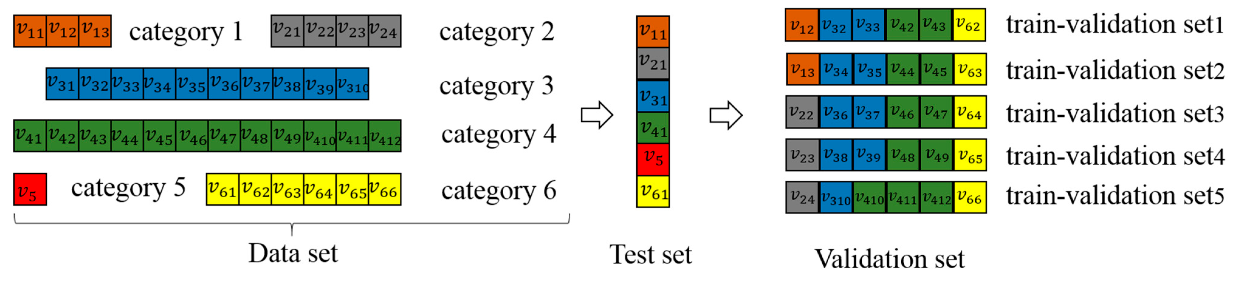
2.3.2. K-Means Clustering Algorithm and Division of Training–Validation–Test (TVT) Set

Because of the uneven distribution of some datasets, using random data allocation can easily lead to a reduction in the training learning range of the NN model and the maximum and minimum points not fitting well. After clustering, selecting data from different categories to validate and test NN models enhances the models’ credibility. The K-means clustering algorithm randomly selects k points in the data space as clustering centers at first. Then, all points in the data space are divided into different categories depending on the closest distance to these centers. A set of new centers would be calculated as the means of the points in each category. The iterative process would be stopped until the centers are unchangeable. Data within each category have the same properties.
Through clustering, we selected one point from every category to form a test set and completed the same process with the remaining points from every category to form a validation set. In the end, the training set consisted of the remaining points from all categories (Figure 3). To adequately mine a dataset, the number of groups of TVT sets was calculated by:
N g r o u p = i = 1 k C N k 1 n k
N g r o u p is the total number of groups of TVT sets, and N k is the number of points in the k-th category.
Figure 3. Division of TVT sets ( v i j , i stands for the category, and j stands for the serial number in the corresponding category).
Water 16 01132 g003

2.3.3. Fitting Precision

The determined coefficients (R2) and root mean square error (RMSE) were adopted to describe the fitting ability of the NN models as:
R 2 = i L m , i L m ¯ L s , i L s ¯ 2 i L m , i L m ¯ 2 i L s , i L s ¯ 2
R M S E = 1 N i = 1 N L m , i L s , i 2
where L m is the monitoring data, L s is the output of the NN model simulation, and N is the number of data.

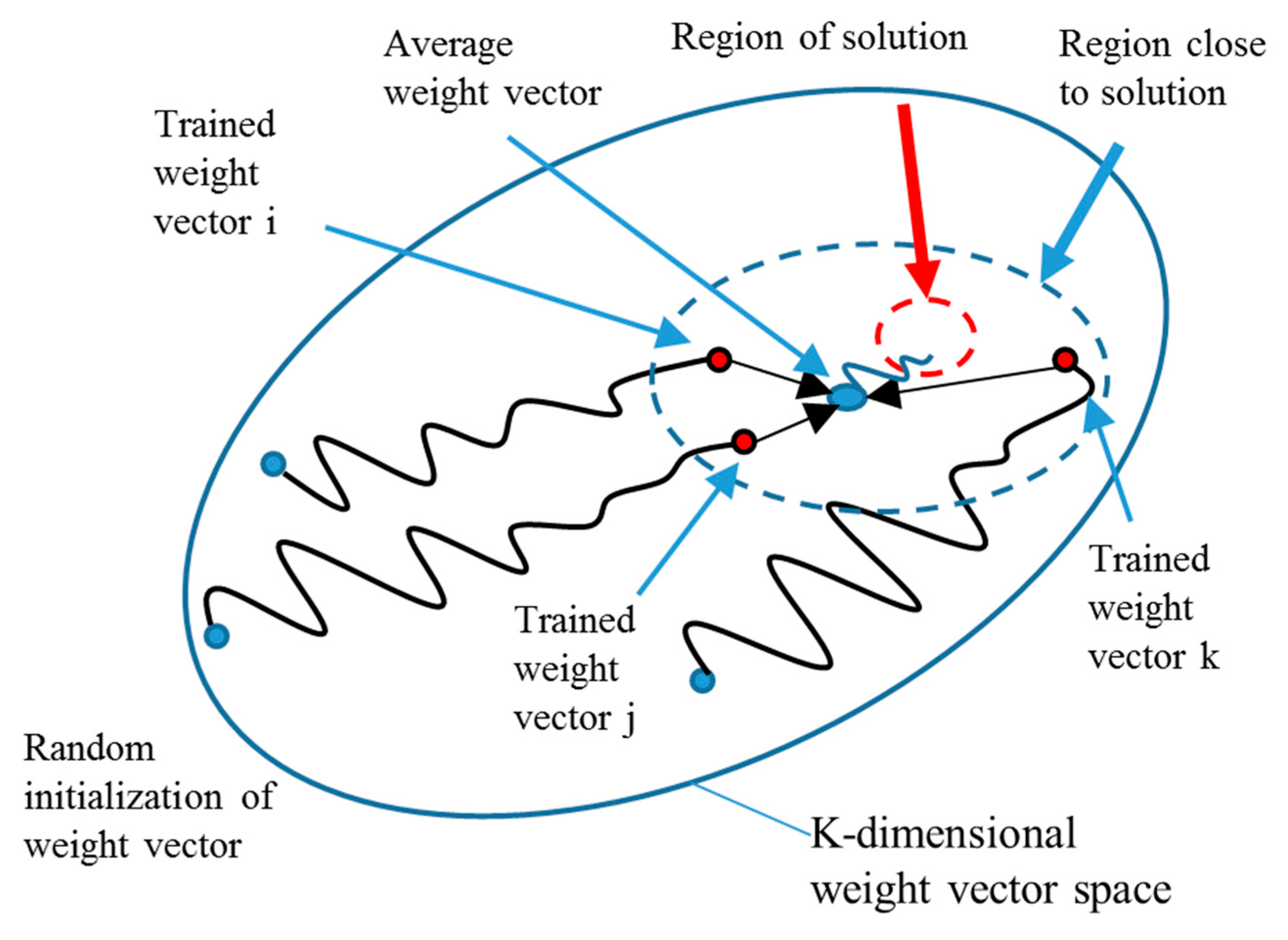
2.3.4. Average Weight Initialization Neural Network

As mentioned in the study by Jinwook Go (2004), the matrixes of an NN model’s weight and bias can be tiled into a vector [42]. The representative vectors that reflect the nonlinear relationships of existing data are located in a specific region of a vector space, as shown by the red dashed area in Figure 3. Even if these weight vectors are not located in the target region of vector space, they belong to a region that is close to the region of the solution, as shown by the blue dashed area in Figure 4. Vectors selected from the region consisting of trained weight vectors can avoid the interference of the local minimum of the training error and ensure that the weights can be effectively approximated to the nonlinear relationship after training.
Based on the principle above, the detailed steps of the average weight initialization algorithm are as follows:
  • Implement the K-means algorithm in the existing dataset and divide the dataset into K categories. The TVT set is divided in the proportion of 70%:15%:15%. The number of groups of the TVT sets is N g r o u p = i = 1 k C N k 1 n k .
  • Train the training sets on the TVT sets. When the accuracy of the training–validation sets is up to standard, subtract the weight of the trained BPNN model as follows:
W i = W i | R t r a i n v a l i d a t e 2 W i | g r o u p i R c o n s t a i n 2
W i = W i | R M S E t r a i n v a l i d a t e W i | g r o u p i R M S E c o n s t r a i n
where W i is the weight of the trained NN model in the i-th group. R t r a i n v a l i d a t e 2 and R M S E t r a i n v a l i d a t e are the accuracies of the training set and the validation set in the trained NN model. R c o n s t a i n 2 and R M S E c o n s t r a i n are the limits of the accuracy of the training set and validation set in the trained NN model.
3.
Average the weights of the trained models:
W a v g i n i t i a l = 1 N g r o u p i = 1 N g r o u p W i
where W a v g i n i t i a l is the averaged weight and N g r o u p is the number of groups of TVT sets.
4.
Divide the existing dataset into k TVT sets. The average weight in step (3) is applied as the initial weight to train and validate the NN models by the k TVT sets. The k-fold cross-validation method is used to assess the performance of the average weight initialization algorithm. The process stops when the accuracy in the test set reaches the standard of accuracy.
5.
The average of the k models’ outputs can be used as the total output of the AWINN model.

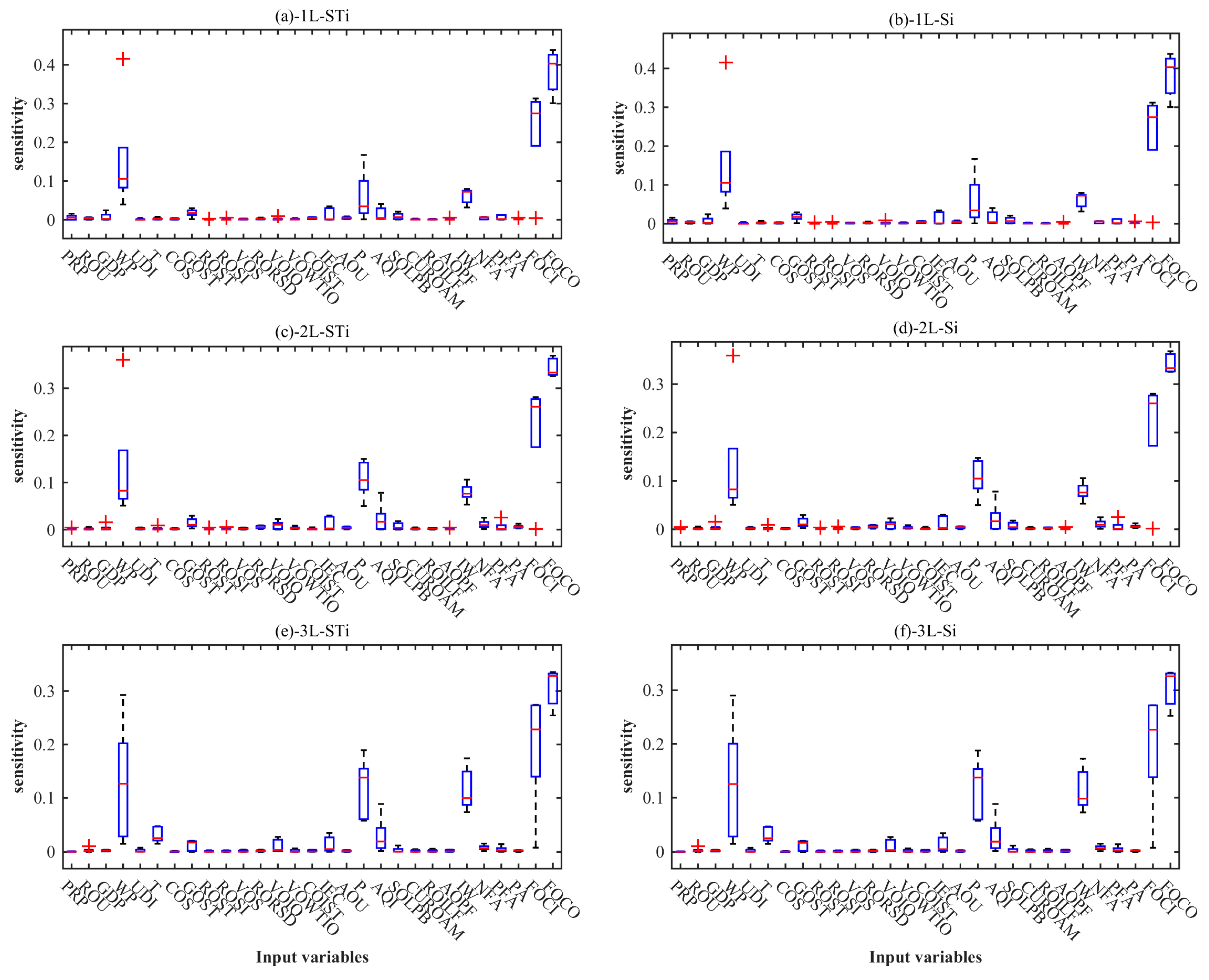
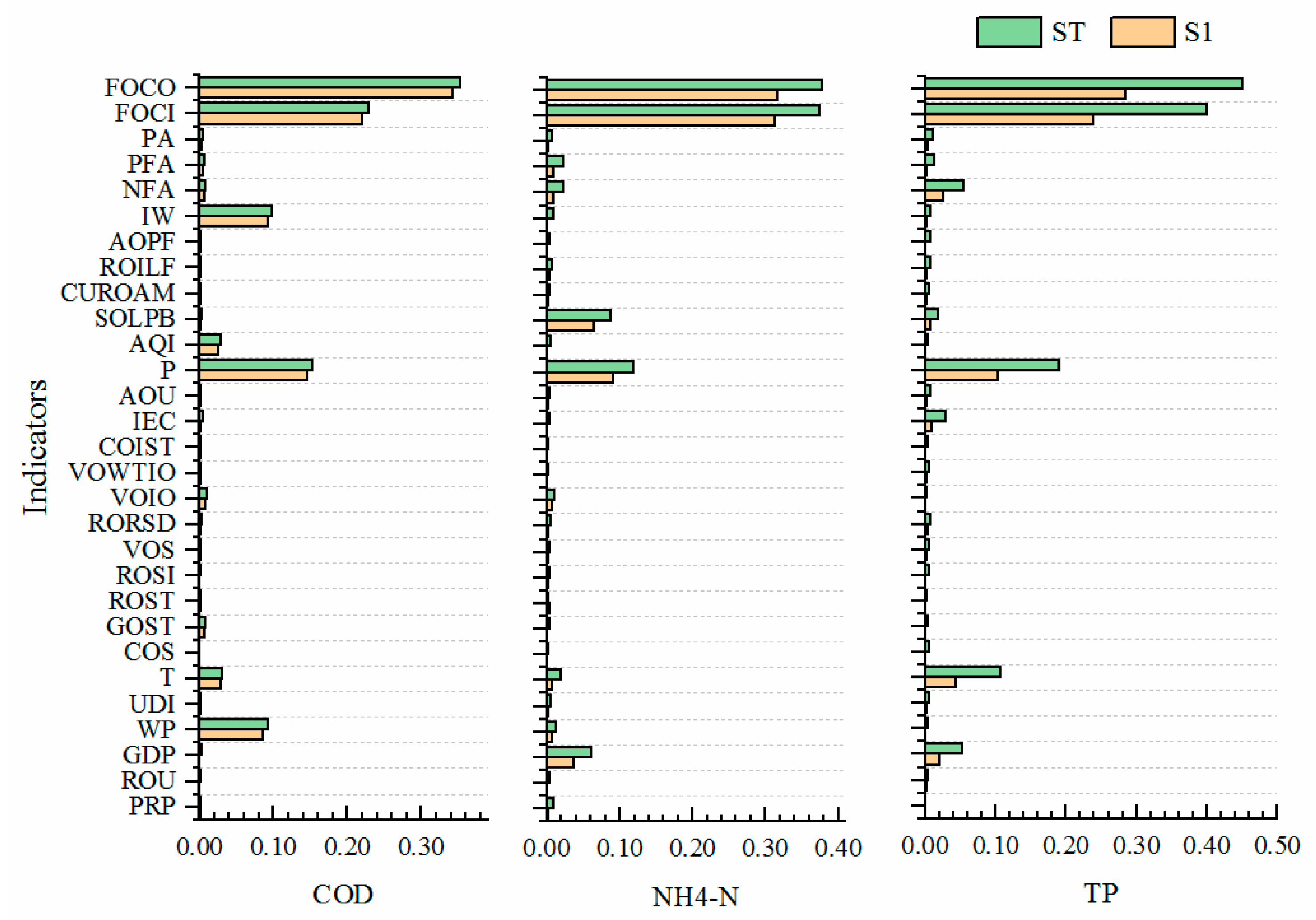
2.3.5. Sobol Sensitivity Analysis

Sobol sensitivity analysis is a global sensitivity analysis method [46]. The method randomly generates input data using Latin hypercube sampling (LHS) and calculates sensitivity by the output value variance. According to the size of the input of the NN models, the LHS method generates two input datasets. When the i-th parameter’s sensitivity is explored, the parameter value in the two datasets is exchanged, and two new datasets are formed. The output values calculated by the investigated models can be combined to calculate the variances. Last, the first-order, second-order, and total sensitivity can be calculated as follows [49]:
  • First-order sensitivity coefficient ( S i ) : standing for the sole influence of a single input parameter x i :
    S i = V x i E ~ i Y | X i V Y
  • Second-order sensitivity coefficient ( S i , j ) : standing for the joint influence of two input parameters x i and x j :
    S i , j = V x i x j E ~ i j Y | X i , X j V x i E ~ i Y | X i V x j E ~ j Y | X j V Y
  • Total sensitivity coefficient ( S T i ) : standing for all of the influences, including a single input parameter x i :
S T i = 1 V x ~ i E ~ i Y | X ~ i V Y
where V Y is the variance of the unchanged input dataset’s output, V x i E ~ i Y | X i is the variance of output expectation that corresponds to input datasets exchanging i-th parameter value x i , V x i x j E ~ i j Y | X i , X j is the variance of the output expectation that corresponds to the input dataset exchanging i-th and j-th parameter values x i and x j . V x ~ i E ~ i Y | X ~ i is the variance of the output expectation that corresponds to the input dataset but not exchanging i-th parameter value x i .

2.3.6. Methods of Overfitting Prevention

The particle swarm optimization neural network (PSONN) is a modified NN model that trains datasets with the help of the PSO algorithm. The weight vector is a particle in the algorithm. A swarm of particles is randomly generated, and the swarm evolves by selecting the best particle and updating the best particle in an iterative process. The iteration stops after satisfying some criterion, and the final best particle is selected as the weight and bias of the post-trained NN model. Generally, the PSONN model can overcome the local minimum and is a classical training algorithm that has been proven to reduce the influence of overfitting. The detail of the algorithm can be seen in the source paper [33].
AdaboostR is an important ensemble learning algorithm suitable for small dataset data mining. Adaboost regression (AdaboostR) is used for regression problems. The algorithm can adopt the abilities of multiple weak learning machines to learn unbalanced data. Combined with BPNN models, the algorithm can detect the error of the trained weak BPNN model in the validation set. Compared to PSONN, it is also a good choice to solve overfitting from a different angle. Details about AdaboostR can be seen in the source paper [28].

3. Results

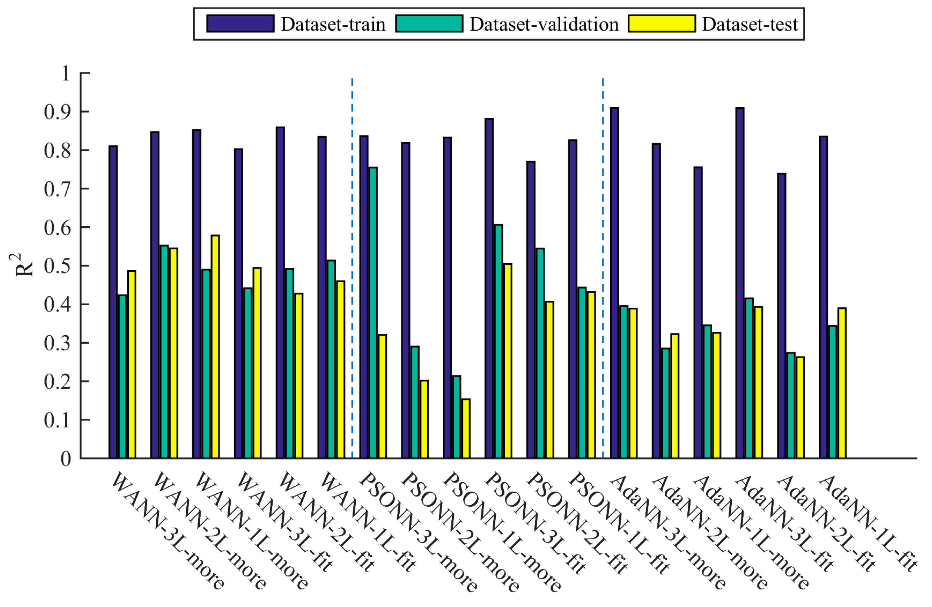
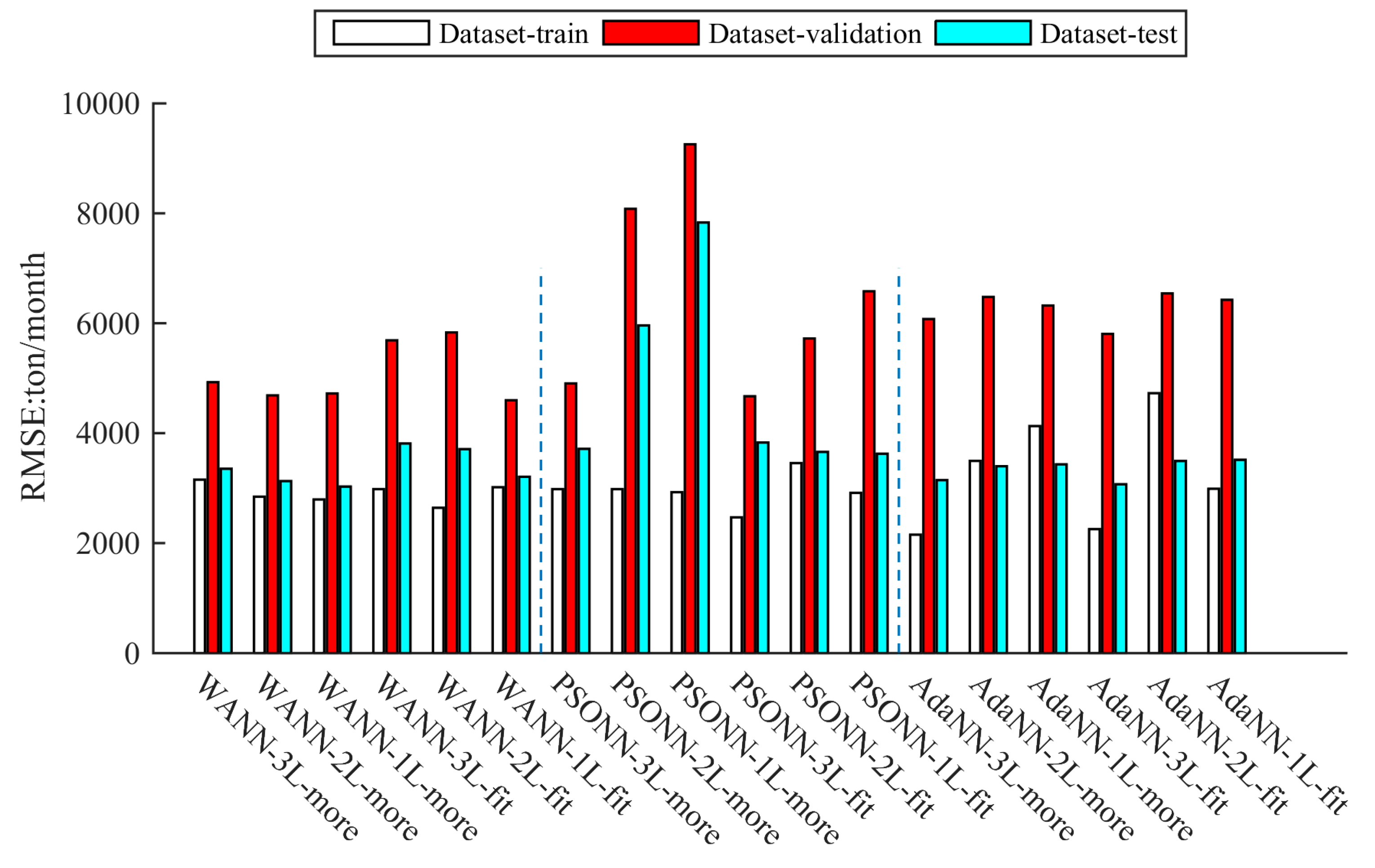
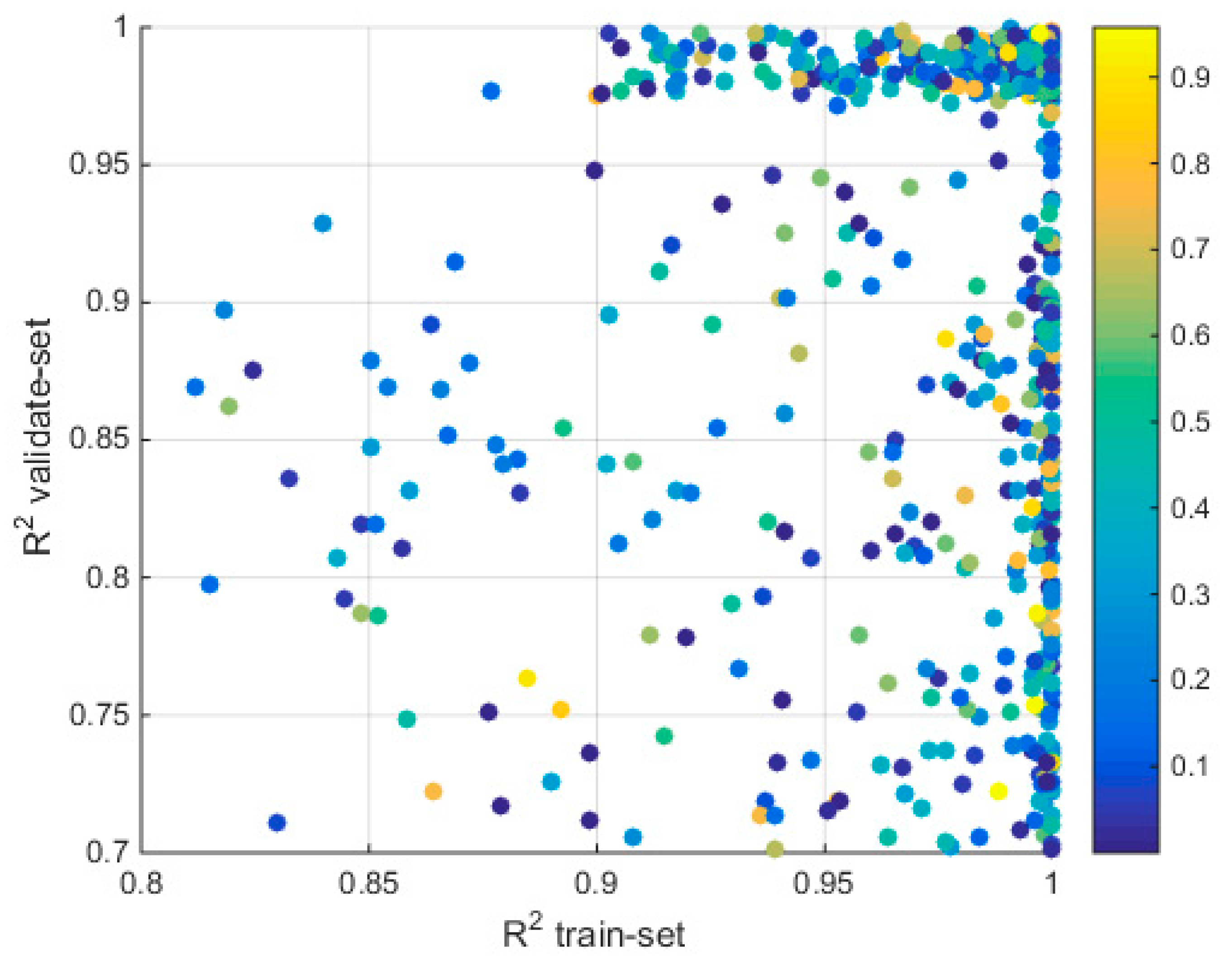
3.1. Comparison of Different Algorithms’ Fitting Accuracy

In this study, the models’ performances were compared according to the NN models’ structure set in Table 1. The R2 and RMSE were used to compare the accuracy of the COD load data fitting in the AWINN, PSONN, and AdaboostR models, with different numbers of hidden layers and neuron numbers in each hidden layer. Figure 5 and Figure 6 show the results. It was found that (1) compared to the PSONN and AdaboostR models, the accuracy of the AWINN models in the test set was higher. The results of the R2 of the AWINN models were in the range of 0.42 to 0.57. The results of the RMSE were in the range of 3027 to 3811 (t/mon). The best R2 performance of the PSONN models was 0.5, and 0.39 for the AdaboostR models. The best RMSE performance of the PSONN models was 3625 (t/mon) and 3071 (t/mon) for the AdaboostR models. According to the study by Schoner (1992) [50], it is difficult to reach a balance in the accuracy of training, validation, and test datasets. The accuracy of the test set in the interval between 0.4 and 0.6 was acceptable. (2) The increase in the number of hidden layers of the NN models may have contributed to the accuracy of the test set. The number of hidden layers had a significant influence on the PSONN models, and models with more hidden layers reached higher accuracy. (3) As for the issue of the number of neurons in the hidden layers, the setting rules only affected the results of PSONN. It was proven that the AWINN method has strong applicability.
The loads of Nh4-N and TP were also modeled by the AWINN models, with three hidden layers. The accuracy in the test set was 0.84 and 0.51 in R2, and 143.94 t/mon and 43.23 t/mon in RMSE. High fitting accuracy was obtained. This shows that the AWINN model can produce high fitting accuracy under the conditions of different output indicators.

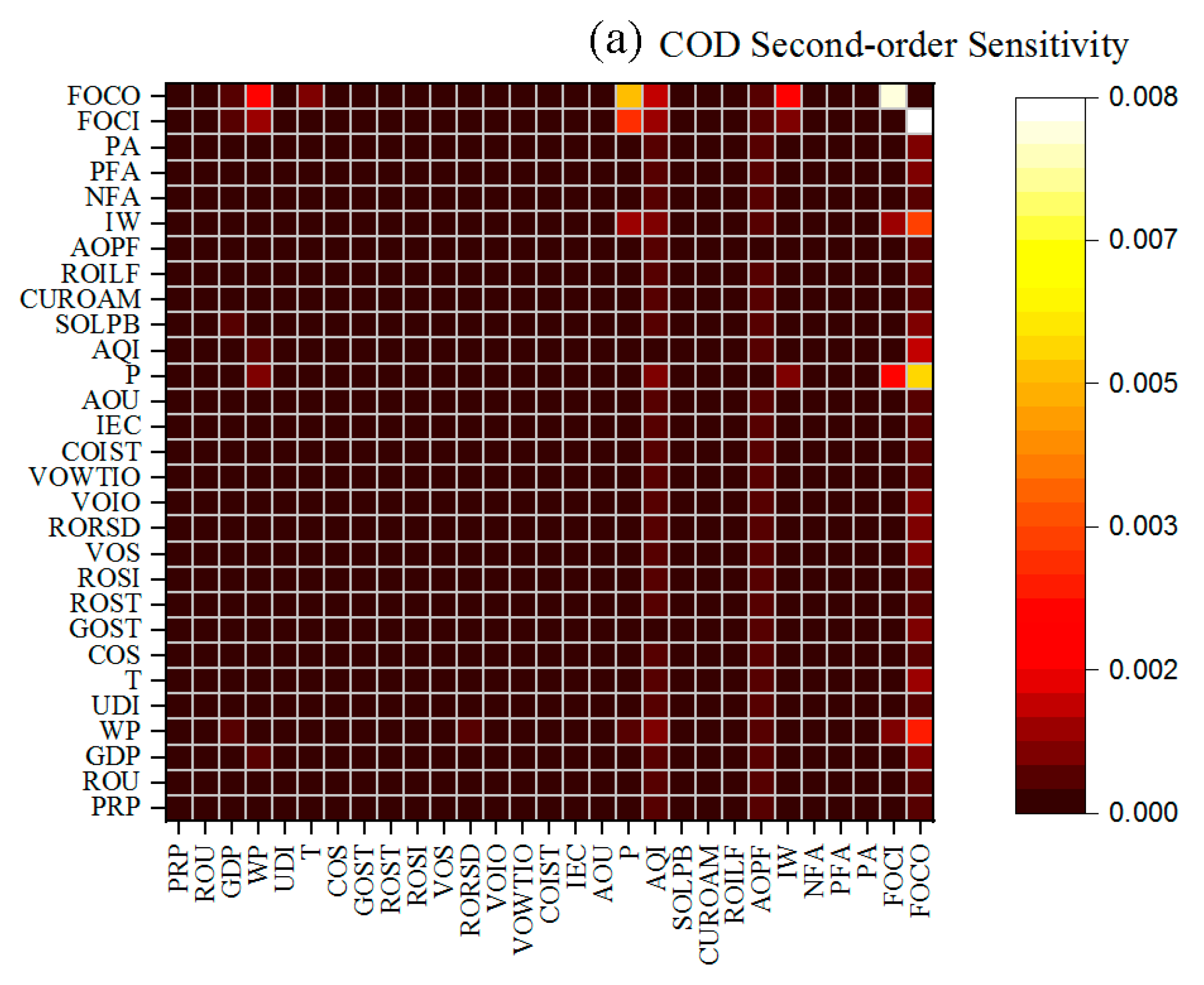
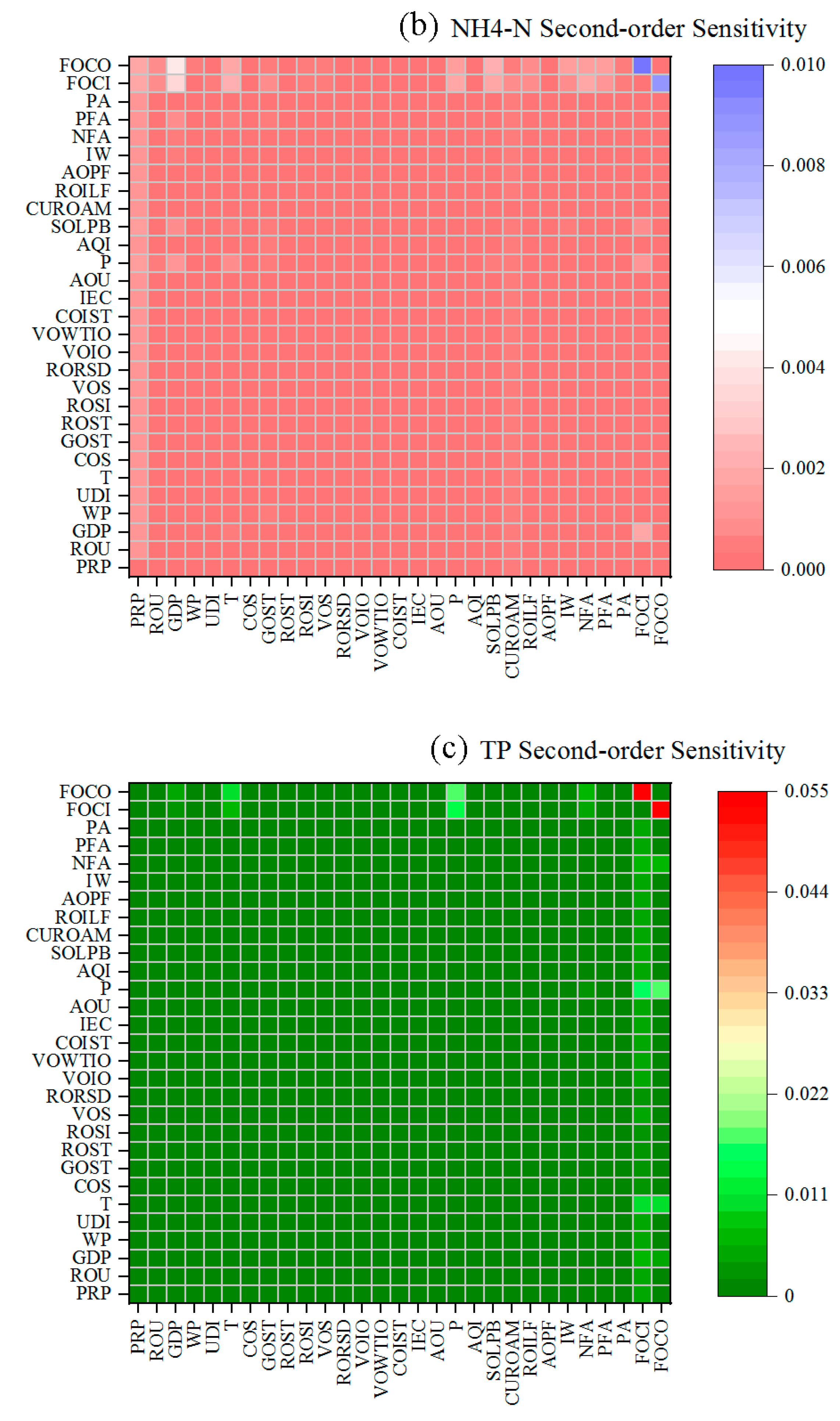
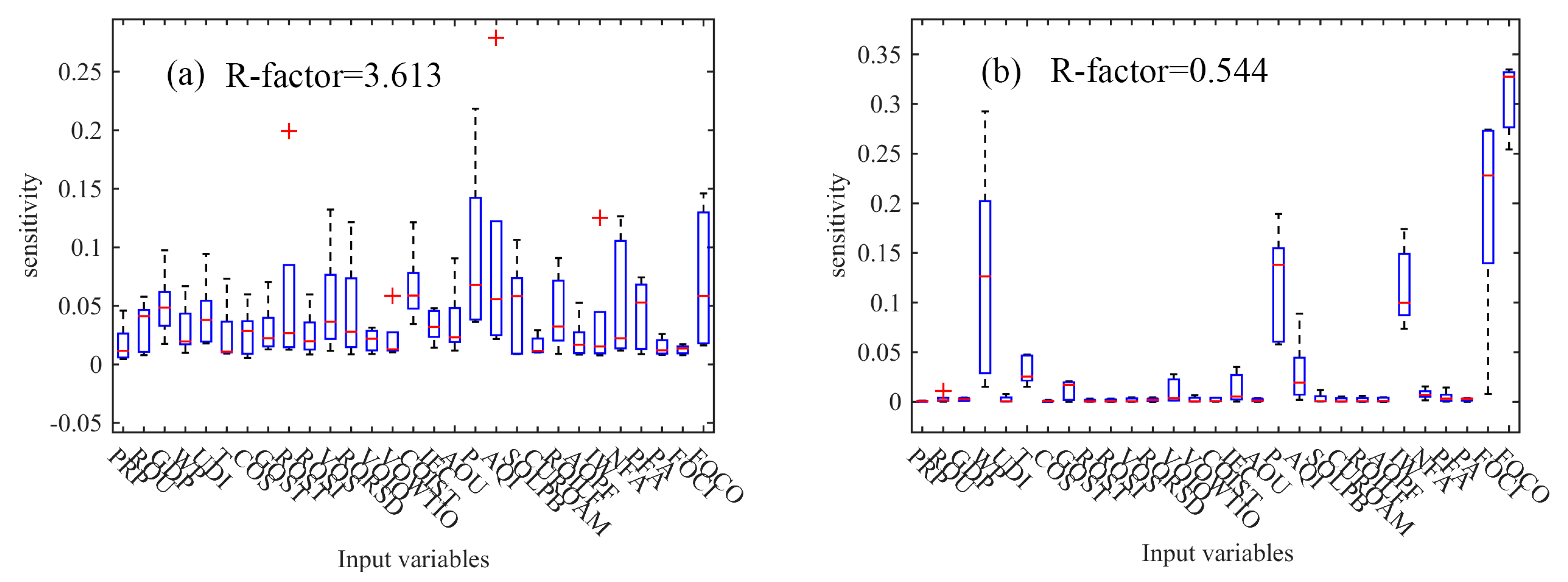
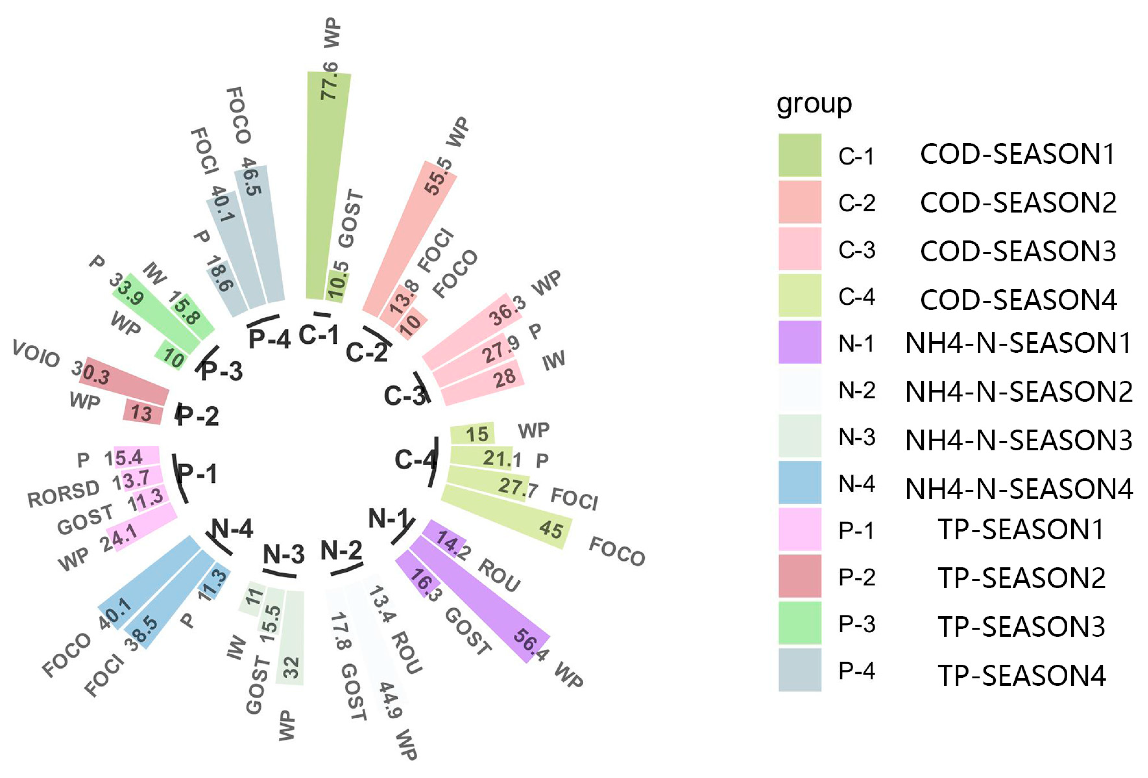
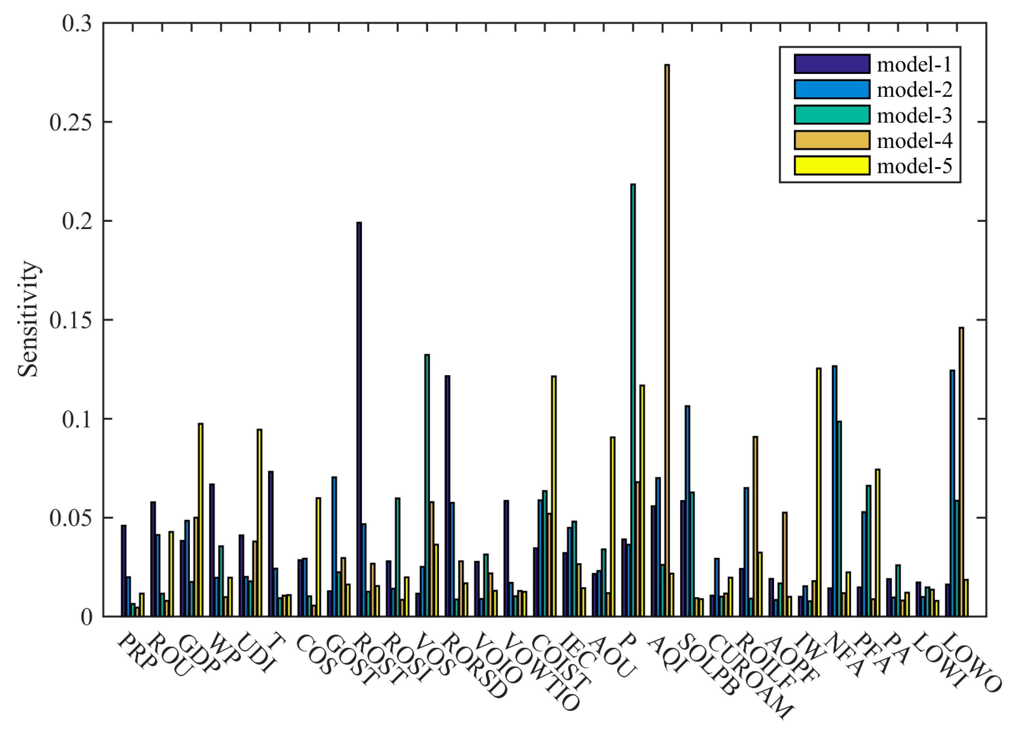
3.2. Results of Sensitivity Analysis

For the usage of NN models, the k-fold cross-validation method was adopted. We divided the collected dataset into 5–10 groups of TVT sets for the final application. The Sobol global sensitivity analysis method was used to analyze the sensitivity of the AWINN models with one, two, and three hidden layers that simulated the COD load. The results of sensitivity analysis can be seen in Figure 7 as boxplots.
At the same time, sensitivity analysis was also carried out for the NH4-N and TP models. The index sensitivity results of three types of pollutant load models are shown in Figure 8. The main factors affecting the COD load included WP, P, IW, FOCI, and FOCO. The main factors affecting NH4-N included GDP, P, SOLPB, FOCI, and FOCO. The main factors affecting TP included GDP, T, P, NFA, FOCI, and FOCO.
The results show that the differences between the ST and S1 of the indicators affecting the COD were small, so the joint influence of the indicators affecting the COD was small. There were certain difference values between the ST and S1 of the indicators affecting NH4-N and TP, so there was a combined influence in the two pollutant loads’ models.
By analyzing the second-order sensitivity, the joint influence of various factors affecting the pollution load was analyzed, as shown in Figure 9. The results show that the joint influence of FOCI and FOCO was the most significant indicator pair for the three types of pollutants. The main joint influence of two factors on loads of NH4-N included (GDP, FOCI) and (SOLPB, FOCI). The main joint influence of two factors on loads of TP included (T, FOCO), (T, FOCI), (P, FOCO), (P, FOCI), (NFA, FOCO), and (NFA, FOCI). Other joint influences of the two factors on the load of COD were not significant.

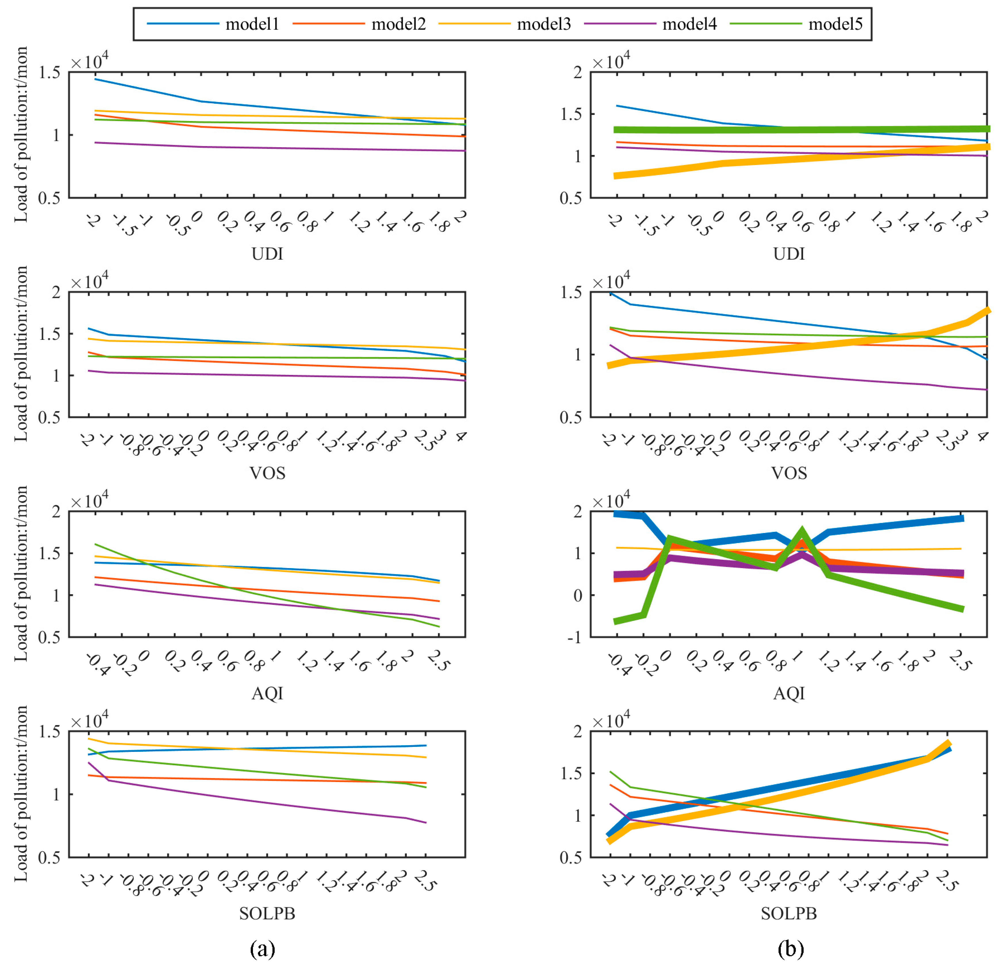
3.3. Results of Model Stability

Through the sensitivity analysis results of the AWINN models with different hidden layers, it was found that the sensitivity results of the models with three hidden layers did not display any exceptional data points, which means the model was more stable.
To effectively evaluate the stability of these models, the R-factor was used in this study:
R f a c t o r = S p S x ¯
S p is the average value of the difference of the quantiles of the sensitivity results of each index, and S x ¯ is the standard deviation of the average value of the results of each index. When the R-factor value is less than 1, the smaller the value, the higher the stability of the model.
Based on the random weight initialization NN model and the proposed AWINN model, the indicator sensitivity results of the five models trained in the five-fold cross-validation dataset were obtained. The results show that the index sensitivity of the weighted average initialization model was more consistent than that of the sensitivity analysis obtained from the randomly initialized weighted NN model, as shown in Figure 10. This shows that the AWINN model was more stable. As the indicator described, it was found that the R-factor value of the AWINN model was 0.544, and the R-factor value of the BPNN model with random weight initialization was 3.613, indicating that the AWINN model was more stable.

4. Discussion

Although the low-sensitivity indicator has little influence on the output of the model, whether the model output changes stably with the low-sensitivity indicator reflects the performance of the model in practice. Based on the five-fold cross-validation dataset, this study analyzed the changes in the output of models with one and three hidden layers caused by the increase in low-sensitivity indicators such as UDI, VOS, AQI, and SOLPB. It can be seen from Figure 11 that the outputs of the three-hidden-layer NN models changing with the low-sensitivity index were more consistent than those of the single-hidden-layer models. This indicates that the model obtained from the training of the three-hidden-layer NN models on different datasets was better able to capture the inherent nonlinear mechanism of these models. This shows that the AWINN model was more stable and reliable under the condition of multiple hidden layers.
The results of the sensitivity analysis show that FOCI, FOCO, and P were the most important factors affecting the three types of pollutant load. It can be inferred that the pollution load in the Xiangyang section of the Hanjiang River catchment is greatly affected by the variation of rainfall and sink discharge. Through single-indicator and double-indicator scenario analysis, it was found that an increase in the three factors would lead to an increase in pollutant loads. However, according to a study by Yonggui Wang (2016), an increase in water volume would lead to an increase in water environmental capacity, thus reducing the risk of exceeding water quality [51]. According to the study by Cheng et al. (2021), the flow in the Xiangyang section of the Hanjiang River has the greatest impact on water quality, which also confirms the fact that the inlet and outlet flow have great impacts [52].
Human activities such as industrial and agricultural production and natural conditions are usually different in different seasons. Identifying the main factors that affect the generation of pollution load in different seasons is of great significance for controlling pollution load. Therefore, this study explored the main factors affecting the pollution load in the catchment in different seasons through Sobol sensitivity analysis. In this study, the year was divided into the first, second, third, and fourth seasons according to January–March, April–June, July–September, and October–December, respectively. The indicators of greater total sensitivity in each season are shown in Figure 12.
It can be seen that after the seasonal analysis, the number of main factors affecting different pollution loads increased, such as the influence of WP and GOST on the three pollutant loads. At the same time, it was found that IW in the third season was the main influencing factor for the three pollutant loads. This is because the main irrigation period in the Xiangyang area is concentrated in the third season. Paddy field irrigation is the main irrigation field, so we should pay attention to the irrigation management of paddy fields. This finding was difficult to detect in the full-time analysis. The impact in the fourth season is more consistent with the full year. From the first season to the fourth season, the impact of WP on the three pollutant loads gradually decreased, and the impact of FOCI and FOCO gradually increased. This indicates that the impact of human activity was more significant in the first three seasons of the catchment. For the influence of human activities to be intensified, we should pay attention to the influence of controllable human activity factors in different seasons, such as WP, COS, CUROAM, IW, and FA.
The results of the full-time second-order sensitivity analysis were compared with those of the seasonal second-order sensitivity analysis, as shown in Figure 13. In the third season, there always existed a joint influence between IW and other factors that affected the three pollutant loads. The results of the second-order sensitivity analysis in the fourth season were similar to those of the all-time analysis. It was found that WP had a high sensitivity to the joint influence on COD load in each season of the year. This phenomenon was difficult to find in previous single-indicator sensitivity research, in which WP was regarded as a secondary influencing factor. Among the second-order sensitivity of NH4-N in the first season, AQI in the first season had a significant impact. Through analysis of historical data, it was found that AQI in the first season was usually the worst in the whole year. This could be an important reason why air quality affects the NH4-N load. In the results of the second-order sensitivity analysis of the TP model, sewage treatment-related indicator pairs had high sensitivity in the first three seasons.
Finally, we should say that there are still some limitations in this study. (1) Due to the lack of detailed data, it was difficult to explore the spatial variation of pollution load within the catchment. This needs to be achieved in the future with spatial data interpolation, remote sensing data, and more data monitoring. (2) Future studies can also be explored in the field of data enhancement to make machine learning models more effective.

5. Conclusions

In this paper, aiming at solving the instability of the BPNN model under the condition of random weight initialization and data scarcity, the AWINN model is proposed for simulating the nonlinear relationship between pollutant loads and factors within the Xiangyang section of the Hanjiang River catchment. The model can improve the stability of multi-index integrated prediction of catchment pollutant load. Compared with the results of the AdaboostR model and PSONN model, the AWINN model has higher accuracy than the other two models. The AWINN model significantly improves the stability of the NN model. Different numbers of hidden layers and hidden-layer neurons were investigated. The addition of the hidden layers of the NN model can increase the stability of the integrated prediction.
Through global sensitivity analysis, the main factors affecting three pollutant loads of COD, NH4-N, and TP are identified, which mainly include the flow of the catchment inlet, the flow of the catchment outlet, and precipitation. It is also confirmed that water volume is the main factor affecting pollutant load in this catchment. At the same time, the combinations of indicators that affect the loads of different pollutants are different. The temporal variation of factors that affect pollutant loads across seasons is manifested in the influence of water price on three types of pollutants and the grade of sewage treatment on NH4-N. The main effect in the third season should focus on the irrigation water. This study provides a more stable method for the integrated prediction of catchment water pollution while enabling quantitative analysis for the attribution of different factors for the pollutant load within a catchment.

Author Contributions

Conceptualization, D.M. and D.S.; methodology, D.M.; software, D.M.; validation, W.G., D.M. and W.L.; formal analysis, J.L.; resources, W.H. and J.F.; writing—review and editing, D.M.; funding acquisition, D.S. All authors have read and agreed to the published version of the manuscript.

Funding

This work was supported by the National Natural Science Foundation of China (No. U21A20156).

Data Availability Statement

The data presented in this study are available on request from the corresponding author. The data are not publicly available due to the requirements of superior management.

Acknowledgments

The authors are thankful to the National Natural Science Foundation of China for the generous funding under project No. U21A20156. Moreover, we are highly grateful to the authors, corporations, and organizations whose material was utilized in the preparation of this article.

Conflicts of Interest

The authors declare no conflicts of interest.

Appendix A. Monthly Data Collection and Data Processing of Input Factors

According to the actual situation, only some factors had monthly monitoring data, while the data of the remaining factors were derived according to relevant rules. Now the situation of each input factor is introduced:
Population, urbanization rate, and urban area: Linear interpolation is performed between two years according to the statistical values at the end of each year.
GDP, disposable income, industrial output value, and industrial electricity consumption: Except for the months with monthly statistics, the remaining months are calculated on average within the quarter according to the statistical values of the corresponding quarter and year.
Water price: The overall water price is summarized monthly based on the water price data released by each county in Xiangyang City.
Sewage treatment capacity and sewage treatment grade: According to the treatment scale and completion and the operation time of sewage treatment plants built, operated, and reconstructed in Xiangyang City since 1980, it is sorted out and updated on a monthly basis.
Sewage treatment rate: This represents the monthly sewage treatment rate of the current year based on the sewage treatment rate in the annual statistical yearbook.
Sewage interception rate, rainwater, and sewage separation rate: The length of sewer pipes built in Xiangyang City since 1980 is counted, the length of sewage collection pipes and rainwater pipes is counted every year, and the proportion of sewage collection pipe length and rainwater pipe length is updated monthly.
Proportion of output value of service industry: This is calculated according to the ratio of the output value of the service industry to the GDP in the annual statistical yearbook, and it is used as the ratio of the output value of service industry in each month of the year.
Water consumption of CNY 10,000 of industrial added value: According to the statistical data of the Hubei Provincial Water Resources Bulletin, the statistical value of the current year is calculated as the monthly water consumption value of the current year.
Rainfall and climatic conditions: The overall average value is calculated based on the monitoring data of rainfall and temperature from six meteorological stations in Xiangyang in the China Meteorological Data Network.
Air-quality index: monthly air quality index data from the China Air Quality Monitoring Network.
Breeding quantity: according to the Hubei Rural Statistical Yearbook on the four categories of pig, cattle, sheep, and poultry stock and the market conversion into pig equivalent for calculation, and according to the year-end stock and the year of the market to calculate the breeding stock of the year.
Comprehensive utilization rate of manure: based on relevant statistics from the Hubei Rural Statistical Yearbook and the Xiangyang Statistical Yearbook, and used as monthly values within the year.
Large-scale breeding rate: The large-scale breeding coefficient is obtained by summing the ratio of the four types of large-scale breeding volume of pigs, cattle, sheep, and poultry to the total stock.
Paddy field area: According to the Hubei Rural Statistical Yearbook, the paddy field area is counted as the paddy field area value for each month of the year.
Nitrogen fertilizer and phosphate fertilizer: The monthly fertilizer application amount is calculated by multiplying the standard usage amount of major crops of wheat, rice, rape, corn, and vegetables in each month with the planting area of each crop, and scaling according to the final annual application amount.
Pesticide quantity: The monthly average value of pesticide application according to the Hubei Rural Statistical Yearbook is used as the value of pesticide application in each month of the year.
Irrigation process: According to the monitoring situation of the Xiangyang Changqu irrigation area, rice is irrigated only in the sixth, seventh, eight, and ninth months, and the farmland obtains water through natural precipitation in the other months. Therefore, January to May and October to December of each year are set as the non-irrigation period, and June to September is the irrigation period. According to the process of rice water consumption in the Changqu irrigation area, the required irrigation water amount during the irrigation period is calculated in combination with the annual monthly precipitation.
Outlet and inlet flow: The monthly average flow is calculated from the monthly daily monitoring flow data.

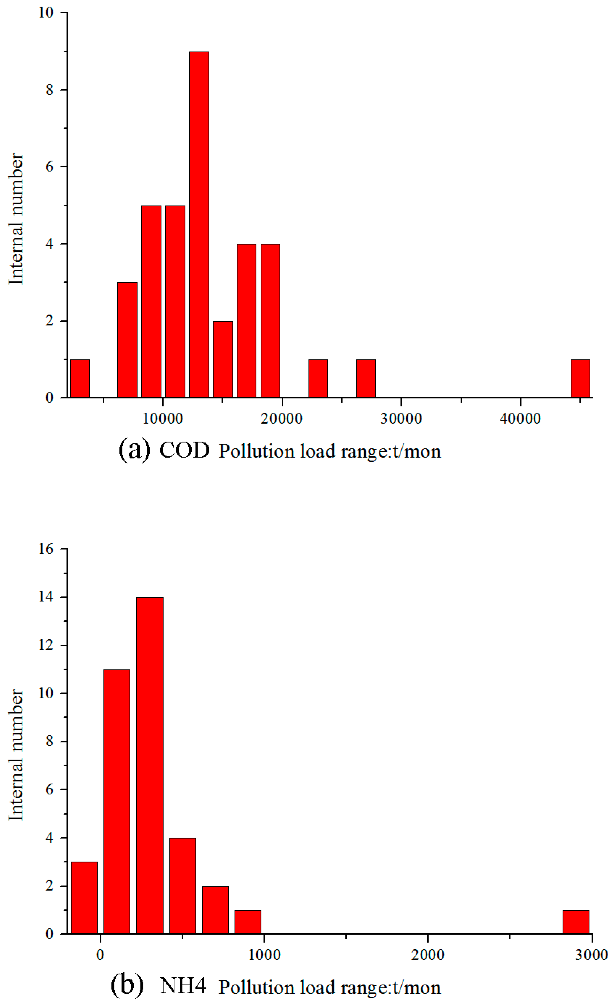
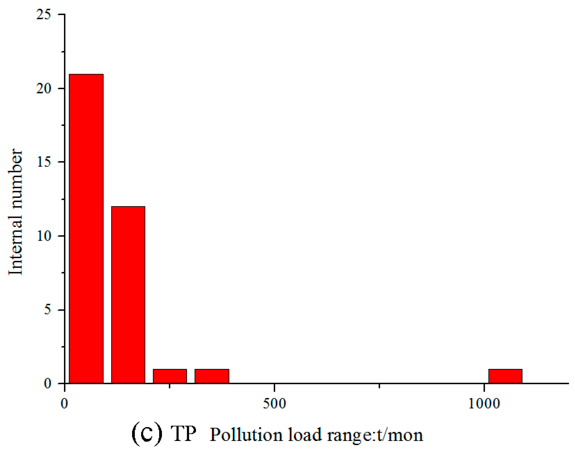
Appendix B. Details of Output Data

According to the load estimation procedure proposed by the USGS, the calculation method of pollutant loads in the river section was applied [53]. The effect of water flow on pollution load reduction was considered in this study. According to the difference of pollutant loads at the outlet and inlet of the basin, the pooled amounts of three pollutant loads of COD, NH4-N, and TP were calculated as shown in Equation (A1).
L m = i = 1 T m o n ( c o u t , i × Q o u t , i j = 1 N c i n , i , j × Q i n , i , j ) × 0.0864
L m is the monthly loads of pollutants ( t / m o n ) , Q o u t , i is the flow of catchment outlet in the i-th day ( m 3 / s ) , c o u t , i is the water quality of the catchment outlet on the i-th day ( m g / L ) , Q i n , i , j is the flow of the catchment inlet on the i-th day ( m 3 / s ) , and c i n , i , j c o u t , i is the water quality of the catchment outlet on the i-th day ( m g / L ) .
By analyzing the monthly load distribution of different pollutants (see Figure A1), it can be seen that 88.9% of the COD load was distributed in the range of 6000–20,000 (t/mon), 91.7% of the NH4-N load was distributed in the range of 0–6000 (t/mon), and 69.4% of the TP load was distributed in the range of 0–200 (t/mon). However, there were few large and small values, which shows that the data distribution was imbalanced. This will also affect the performance of machine learning in the imbalanced part.
Figure A1. The distribution of pollutants loads: (a) COD; (b) NH4-N; (c) TP.
Water 16 01132 g0a1aWater 16 01132 g0a1b

Appendix C. Overfitting and Instability of the Random Weight Initialization BP Algorithm

Based on the data set of this study, the BP NN was trained and verified. After uncertain times of training and verification, a model with training and verification standards (R2 of the training set is greater than 0.8 and R2 of the validation set is greater than 0.7) was obtained. By analyzing the accuracy of the test set of 710 trained and verified models reaching the target (see Figure A2), we found that the results of the test set were unstable and did not present a regular distribution. This raises the question of whether the model that meets the test set the one that can be trusted.
Figure A2. Test set fit accuracy (training and validation accuracy is up to standard).
Water 16 01132 g0a2
The five data sets divided by the clustering algorithm in Section 2.3.2 were trained several times by random weight initialization, and five models that met the requirements of training, validation, and testing accuracy were obtained. If the outputs of the models are consistent under the condition of the same input, it indicates that the models are reliable. The results of the sensitivity analysis can also illustrate the consistency of the output, so the sensitivity outputs of these models were analyzed, and it was found that the sensitivity outputs of the five models were inconsistent. The result can be seen in Figure A3. This shows that the model trained by random weight initialization was still unstable when the accuracy of the training set, validation set, and test set were up to the standard. This also reflects the defect of the random weight initialization NN model under the condition of data scarcity.
Figure A3. Sensitivity analysis of BPNN models with the training set, validation set, and test set satisfying accuracy requirements.
Water 16 01132 g0a3

References

  1. Deletic, A.; Wang, H. Water Pollution Control for Sustainable Development. Engineering 2019, 5, 839–840. [Google Scholar] [CrossRef]
  2. Bowes, B.D.; Wang, C.; Ercan, M.B.; Culver, T.B.; Beling, P.A.; Goodall, J.L. Reinforcement learning-based real-time control of coastal urban stormwater systems to mitigate flooding and improve water quality. Environ. Sci. Water Res. Technol. 2022, 8, 2065–2086. [Google Scholar] [CrossRef]
  3. Najah Ahmed, A.; Binti Othman, F.; Abdulmohsin Afan, H.; Khaleel Ibrahim, R.; Ming Fai, C.; Shabbir Hossain, M.; Ehteram, M.; Elshafie, A. Machine learning methods for better water quality prediction. J. Hydrol. 2019, 578. [Google Scholar] [CrossRef]
  4. Liu, J.; Dietz, T.; Carpenter, S.R.; Alberti, M.; Folke, C.; Moran, E.; Pell, A.N.; Deadman, P.; Kratz, T.; Lubchenco, J.; et al. Complexity of coupled human and natural systems. Science 2007, 317, 1513–1516. [Google Scholar] [CrossRef] [PubMed]
  5. Larsen, T.A.; Hoffmann, S.; Lüthi, C.; Truffer, B.; Maurer, M. Emerging solutions to the water challenges of an urbanizing world. Science 2016, 352, 928–933. [Google Scholar] [CrossRef] [PubMed]
  6. Johnes, P.J. Evaluation and management of the impact of land use change on the nitrogen and phosphorus load delivered to surface waters: The export coefficient modelling approach. J. Hydrol. 1996, 183, 323–349. [Google Scholar] [CrossRef]
  7. Cheng, X.; Chen, L.; Sun, R.; Jing, Y. An improved export coefficient model to estimate non-point source phosphorus pollution risks under complex precipitation and terrain conditions. Environ. Sci. Pollut. Res. Int. 2018, 25, 20946–20955. [Google Scholar] [CrossRef] [PubMed]
  8. Poor, C.J.; Ullman, J.L. Using regression tree analysis to improve predictions of low-flow nitrate and chloride in Willamette River Basin watersheds. Environ. Manag. 2010, 46, 771–780. [Google Scholar] [CrossRef] [PubMed]
  9. Arnold, J.G.; Moriasi, D.N.; Gassman, P.W.; Abbaspour, K.C.; White, M.J.; Srinivasan, R.; Santhi, C.; Harmel, R.; Van Griensven, A.; Van Liew, M.W. SWAT: Model use, calibration, and validation. Trans. ASABE 2012, 55, 1491–1508. [Google Scholar] [CrossRef]
  10. Liu, J.; Zhang, L.; Zhang, Y.; Hong, H.; Deng, H. Validation of an agricultural non-point source (AGNPS) pollution model for a catchment in the Jiulong River watershed, China. J. Environ. Sci. 2008, 20, 599–606. [Google Scholar] [CrossRef] [PubMed]
  11. Chen, K.; Chen, H.; Zhou, C.; Huang, Y.; Qi, X.; Shen, R.; Liu, F.; Zuo, M.; Zou, X.; Wang, J.; et al. Comparative analysis of surface water quality prediction performance and identification of key water parameters using different machine learning models based on big data. Water Res. 2020, 171, 115454. [Google Scholar] [CrossRef] [PubMed]
  12. Heddam, S.; Kisi, O. Extreme learning machines: A new approach for modeling dissolved oxygen (DO) concentration with and without water quality variables as predictors. Environ. Sci. Pollut. Res. Int. 2017, 24, 16702–16724. [Google Scholar] [CrossRef] [PubMed]
  13. Kurniawan, I.; Hayder, G.; Mustafa, H. Predicting Water Quality Parameters in a Complex River System. J. Ecol. Eng. 2021, 22, 250–257. [Google Scholar] [CrossRef] [PubMed]
  14. Li, L.; Jiang, P.; Xu, H.; Lin, G.; Guo, D.; Wu, H. Water quality prediction based on recurrent neural network and improved evidence theory: A case study of Qiantang River, China. Environ. Sci. Pollut. Res. Int. 2019, 26, 19879–19896. [Google Scholar] [CrossRef] [PubMed]
  15. Ye, Q.; Yang, X.; Chen, C.; Wang, J. River Water Quality Parameters Prediction Method based on LSTM-RNN Model. In Proceedings of the 2019 Chinese Control and Decision Conference (CCDC), Nanchang, China, 3 June 2019; pp. 3024–3028. [Google Scholar]
  16. Yu, J.W.; Kim, J.S.; Li, X.; Jong, Y.C.; Kim, K.H.; Ryang, G.I. Water quality forecasting based on data decomposition, fuzzy clustering and deep learning neural network. Environ. Pollut. 2022, 303, 119136. [Google Scholar] [CrossRef] [PubMed]
  17. Zhang, Y.-F.; Fitch, P.; Thorburn, P.J. Predicting the Trend of Dissolved Oxygen Based on the kPCA-RNN Model. Water 2020, 12, 585. [Google Scholar] [CrossRef]
  18. Guo, H.; Huang, J.J.; Zhu, X.; Wang, B.; Tian, S.; Xu, W.; Mai, Y. A generalized machine learning approach for dissolved oxygen estimation at multiple spatiotemporal scales using remote sensing. Environ. Pollut. 2021, 288, 117734. [Google Scholar] [CrossRef]
  19. Hu, W.; Liu, J.; Wang, H.; Miao, D.; Shao, D.; Gu, W. Retrieval of TP Concentration from UAV Multispectral Images Using IOA-ML Models in Small Inland Waterbodies. Remote Sens. 2023, 15, 1250. [Google Scholar] [CrossRef]
  20. Golden, H.E.; Lane, C.R.; Prues, A.G.; D’Amico, E. Boosted Regression Tree Models to Explain Watershed Nutrient Concentrations and Biological Condition. JAWRA J. Am. Water Resour. Assoc. 2016, 52, 1251–1274. [Google Scholar] [CrossRef]
  21. Granata, F.; Papirio, S.; Esposito, G.; Gargano, R.; De Marinis, G. Machine Learning Algorithms for the Forecasting of Wastewater Quality Indicators. Water 2017, 9, 105. [Google Scholar] [CrossRef]
  22. Lek, S.; Guiresse, M.; Giraudel, J.-L. Predicting stream nitrogen concentration from watershed features using neural networks. Water Res. 1999, 33, 3469–3478. [Google Scholar] [CrossRef]
  23. Li, S.; Cai, X.; Emaminejad, S.A.; Juneja, A.; Niroula, S.; Oh, S.; Wallington, K.; Cusick, R.D.; Gramig, B.M.; John, S.; et al. Developing an integrated technology-environment-economics model to simulate food-energy-water systems in Corn Belt watersheds. Environ. Model. Softw. 2021, 143, 105083. [Google Scholar] [CrossRef]
  24. Liu, M.; Lu, J. Support vector machine-an alternative to artificial neuron network for water quality forecasting in an agricultural nonpoint source polluted river? Environ. Sci. Pollut. Res. Int. 2014, 21, 11036–11053. [Google Scholar] [CrossRef] [PubMed]
  25. Bejani, M.M.; Ghatee, M. A systematic review on overfitting control in shallow and deep neural networks. Artif. Intell. Rev. 2021, 54, 6391–6438. [Google Scholar] [CrossRef]
  26. Ying, X. An Overview of Overfitting and Its Solutions. In Proceedings of the Journal of Physics: Conference Series; IOP Publishing: Bristol, UK, 2019; p. 022022. [Google Scholar]
  27. Srivastava, N.; Hinton, G.; Krizhevsky, A.; Sutskever, I.; Salakhutdinov, R. Dropout: A simple way to prevent neural networks from overfitting. J. Mach. Learn. Res. 2014, 15, 1929–1958. [Google Scholar]
  28. Solomatine, D.P.; Shrestha, D.L. AdaBoost. RT: A Boosting Algorithm for Regression Problems. In Proceedings of the 2004 IEEE International Joint Conference on Neural Networks (IEEE Cat. No. 04CH37541), Budapest, Hungary, 25–29 July 2004; pp. 1163–1168. [Google Scholar]
  29. Bartoletti, N.; Casagli, F.; Marsili-Libelli, S.; Nardi, A.; Palandri, L. Data-driven rainfall/runoff modelling based on a neuro-fuzzy inference system. Environ. Model. Softw. 2018, 106, 35–47. [Google Scholar] [CrossRef]
  30. Jia, W.; Zhao, D.; Zheng, Y.; Hou, S. A novel optimized GA–Elman neural network algorithm. Neural Comput. Appl. 2017, 31, 449–459. [Google Scholar] [CrossRef]
  31. Rohmat, F.I.W.; Gates, T.K.; Labadie, J.W. Enabling improved water and environmental management in an irrigated river basin using multi-agent optimization of reservoir operations. Environ. Model. Softw. 2021, 135, 104909. [Google Scholar] [CrossRef]
  32. Shao, D.; Nong, X.; Tan, X.; Chen, S.; Xu, B.; Hu, N. Daily Water Quality Forecast of the South-To-North Water Diversion Project of China Based on the Cuckoo Search-Back Propagation Neural Network. Water 2018, 10, 1471. [Google Scholar] [CrossRef]
  33. Van den Bergh, F.; Engelbrecht, A.P. A Cooperative Approach to Particle Swarm Optimization. IEEE Trans. Evol. Comput. 2004, 8, 225–239. [Google Scholar] [CrossRef]
  34. Barzegar, R.; Aalami, M.T.; Adamowski, J. Short-term water quality variable prediction using a hybrid CNN–LSTM deep learning model. Stoch. Environ. Res. Risk Assess. 2020, 34, 415–433. [Google Scholar] [CrossRef]
  35. Chen, H.; Chen, A.; Xu, L.; Xie, H.; Qiao, H.; Lin, Q.; Cai, K. A deep learning CNN architecture applied in smart near-infrared analysis of water pollution for agricultural irrigation resources. Agric. Water Manag. 2020, 240, 106303. [Google Scholar] [CrossRef]
  36. Nouraki, A.; Alavi, M.; Golabi, M.; Albaji, M. Prediction of water quality parameters using machine learning models: A case study of the Karun River, Iran. Environ. Sci. Pollut. Res. Int. 2021, 28, 57060–57072. [Google Scholar] [CrossRef] [PubMed]
  37. Bousquet, O.; Elisseeff, A. Stability and generalization. J. Mach. Learn. Res. 2002, 2, 499–526. [Google Scholar]
  38. Narkhede, M.V.; Bartakke, P.P.; Sutaone, M.S. A review on weight initialization strategies for neural networks. Artif. Intell. Rev. 2021, 55, 291–322. [Google Scholar] [CrossRef]
  39. Glorot, X.; Bengio, Y. Understanding the Difficulty of Training Deep Feedforward Neural Networks. In Proceedings of the Thirteenth International Conference on Artificial Intelligence and Statistics, Sardinia, Italy, 13–15 May 2010; pp. 249–256. [Google Scholar]
  40. Nguyen, D.; Widrow, B. Improving the Learning Speed of 2-layer Neural Networks by Choosing Initial Values of the Adaptive Weights. In Proceedings of the 1990 IJCNN International Joint Conference on Neural Networks, San Diego, CA, USA, 17–21 June 1990; pp. 21–26. [Google Scholar]
  41. Go, J.; Lee, C. Analyzing Weight Distribution of Neural Networks. In Proceedings of the IJCNN’99. International Joint Conference on Neural Networks. Proceedings (Cat. No. 99CH36339), Washington, DC, USA, 10–16 July 1999; pp. 1154–1157. [Google Scholar]
  42. Go, J.; Baek, B.; Lee, C. Analyzing Weight Distribution of Feedforward Neural Networks and Efficient Weight Initialization. In Proceedings of the Joint IAPR International Workshops on Statistical Techniques in Pattern Recognition (SPR) and Structural and Syntactic Pattern Recognition (SSPR), Lisbon, Portugal, 18–20 August 2004; pp. 840–849. [Google Scholar]
  43. Akhtar, N.; Syakir Ishak, M.I.; Bhawani, S.A.; Umar, K. Various Natural and Anthropogenic Factors Responsible for Water Quality Degradation: A Review. Water 2021, 13, 2660. [Google Scholar] [CrossRef]
  44. Pastres, R.; Franco, D.; Pecenik, G.; Solidoro, C.; Dejak, C. Local sensitivity analysis of a distributed parameters water quality model. Reliab. Eng. Syst. Saf. 1997, 57, 21–30. [Google Scholar] [CrossRef]
  45. Wang, R.; Kim, J.H.; Li, M.H. Predicting stream water quality under different urban development pattern scenarios with an interpretable machine learning approach. Sci. Total Environ. 2021, 761, 144057. [Google Scholar] [CrossRef] [PubMed]
  46. Razavi, S.; Jakeman, A.; Saltelli, A.; Prieur, C.; Iooss, B.; Borgonovo, E.; Plischke, E.; Lo Piano, S.; Iwanaga, T.; Becker, W.; et al. The Future of Sensitivity Analysis: An essential discipline for systems modeling and policy support. Environ. Model. Softw. 2021, 137, 104954. [Google Scholar] [CrossRef]
  47. LeCun, Y.; Bengio, Y.; Hinton, G. Deep learning. Nature 2015, 521, 436–444. [Google Scholar] [CrossRef] [PubMed]
  48. Moré, J.J. The Levenberg-Marquardt Algorithm: Implementation and Theory. In Numerical Analysis; Springer: Berlin/Heidelberg, Germany, 1978; pp. 105–116. [Google Scholar]
  49. Saltelli, A.; Annoni, P.; Azzini, I.; Campolongo, F.; Ratto, M.; Tarantola, S. Variance based sensitivity analysis of model output. Design and estimator for the total sensitivity index. Comput. Phys. Commun. 2010, 181, 259–270. [Google Scholar] [CrossRef]
  50. Schoner, W. Reaching the generalisation maximum of backpropagation networks. In Artificial Neural Networks; Aleksandr, I., Taylor, J., Eds.; Elsevier: Amsterdam, The Netherlands, 1992; Volume 2, pp. 91–94. [Google Scholar]
  51. Wang, Y.; Zhang, W.; Zhao, Y.; Peng, H.; Shi, Y. Modelling water quality and quantity with the influence of inter-basin water diversion projects and cascade reservoirs in the Middle-lower Hanjiang River. J. Hydrol. 2016, 541, 1348–1362. [Google Scholar] [CrossRef]
  52. Cheng, B.-F.; Zhang, Y.; Xia, R.; Zhang, N.; Zhang, X.-F. Temporal and spatial variations in water quality of Hanjiang river and its influencing factors in recent years. Huan Jing Ke Xue = Huanjing Kexue 2021, 42, 4211–4221. [Google Scholar] [PubMed]
  53. Runkel, R.L.; Crawford, C.G.; Cohn, T.A. Load Estimator (LOADEST): A FORTRAN Program for Estimating Constituent Loads in Streams and Rivers; U.S. Publications Warehouse: Reston, VA, USA, 2004; pp. 2328–7055. Available online: https://pubs.usgs.gov/publication/tm4A5 (accessed on 24 March 2024).
Figure 1. Location of the Xiangyang section of the Hanjiang River catchment (tributary, reservoir, monitoring locations of flow and water quality).
Water 16 01132 g001
Figure 2. The relationships across application methods.
Water 16 01132 g002
Figure 4. Generalized figure of average weight initialization. (The blue dots are weight vectors that are initialized by random initialization. The red dots are weight vectors that are trained by BPNN. The elliptical blue dot is the average weight vector).
Water 16 01132 g004
Figure 5. Comparison of coefficient of determination R2.
Water 16 01132 g005
Figure 6. Comparison of root mean square error (RMSE).
Water 16 01132 g006
Figure 7. First-order and total sensitivity of all factors in different AWINN models with different hidden layer structures: (a) total sensitivity of one-layer AWINN model; (b) first sensitivity of one-layer AWINN model; (c) total sensitivity of two-layer AWINN model; (d) first sensitivity of two-layer AWINN model; (e) total sensitivity of three-layer AWINN model; (f) first sensitivity of three-layer AWINN model. The red plus signs are signals of outliers. Hyphens are quantile number of 50% confidence. Dashed lines are the extension to a bigger or smaller quantile number.
Water 16 01132 g007
Figure 8. First-order and total sensitivity of indicators of COD, NH4-N, and TP models (“ST” is the total sensitivity of each indicator, and “S1” is the first-order sensitivity of each indicator).
Water 16 01132 g008
Figure 9. Second-order sensitivity of indicators of (a) COD, (b) NH4-N, and (c) TP models.
Water 16 01132 g009aWater 16 01132 g009b
Figure 10. Stability results of indicators for (a) random weight initialization NN models; (b) AWINN models. The red plus signs are signals of outliers. Hyphens are quantile number of 50% confidence. dashed lines are the extension to a bigger or smaller quantile number.
Water 16 01132 g010
Figure 11. Outputs of low-sensitivity indicators: (a) three-hidden-layer NN model; (b) single-hidden-layer NN model (bolder lines show abnormal results of single-hidden-layer NN models.).
Water 16 01132 g011
Figure 12. Total sensitivity map by season.
Water 16 01132 g012
Figure 13. Seasonal second-order sensitivity: (a) COD; (b) NH4-N; (c) TP.
Water 16 01132 g013
Table 1. Related factors in the input dataset (variables with monthly monitoring data are identified by the asterisk symbol).
CategoryRelated Factor
Point source
of urban life
Permanent resident population (PRP), gross national product * (GDP), rate of urbanization (ROU), water price * (WP), urban disposable income * (UDI), temperature * (T), capacity of sewage treatment plant * (COS), grade of sewage treatment * (GOST), rate of sewage treatment (ROST), rate of sewage interception * (ROSI)
Point source
of industry
Value of industrial output * (VOIO), volume of water by CNY 10,000 industrial output (VOWTIO), capacity of industrial sewage treatment (COIST), industrial electricity consumption * (IEC), value of service industry output * (VOS)
Non-point source of urban lifeArea of urban (AOU), precipitation * (P), ratio of rainwater and sewage diversion * (RORSD), air-quality index * (AQI)
Non-point source of rural lifeRural population (RP), volume of rural life water utilization (VORLWU), precipitation * (P)
Non-point source of plantingArea of paddy field (AOPF), irrigation water (IW), nitrogen fertilizer application (NFA), phosphate fertilizer application (PFA), pesticide application (PA), precipitation * (P)
Non-point source of the breeding industryStock of livestock and poultry breeding (SOLPB), rate of intensive livestock farm (ROILF), comprehensive utilization rate of aquaculture manure (CUROAM), precipitation * (P)
Pollutant reaction in channelFlow of catchment inlet * (FOCI), flow of catchment outlet * (FOCO)
Table 2. Source of collected data.
Related FactorSource
PRP, ROU, WP, COS, GOST, ROST, ROSI, COIST, AOU, RORSDStatistical Yearbook of Xiangyang City 1980–2020
AOPF, NFA, PFA, PA, SOLPB, ROILFRural Yearbook of Hubei Province 2015–2020
GDP, UDI, VOIO, IECXiangyang City statistics monthly report January 2015–December 2017
AQIPM2.5 historical data website https://www.aqistudy.cn/historydata/ (accessed on 1 January 2015)
T, PChina meteorological data website http://data.cma.cn/ (accessed on 1 January 2015)
FOCI, FOCOOfficial website of Hubei Water Conservancy Department https://slt.hubei.gov.cn/ (accessed on 1 January 2015)
Water quality (WQ)Water Resources Department of Hubei Province
Disclaimer/Publisher’s Note: The statements, opinions and data contained in all publications are solely those of the individual author(s) and contributor(s) and not of MDPI and/or the editor(s). MDPI and/or the editor(s) disclaim responsibility for any injury to people or property resulting from any ideas, methods, instructions or products referred to in the content.

