Article

Combining Crop and Water Decisions to Manage Groundwater Overdraft over Decadal and Longer Timescales

1
Center for Watershed Sciences, University of California, Davis, One Shields Avenue, Davis, CA 95616, USA
2
Department of Civil and Environmental Engineering, University of California, Merced, 5200 North Lake Road, Merced, CA 95343, USA
*
Author to whom correspondence should be addressed.
Water 2024, 16(9), 1223; https://doi.org/10.3390/w16091223
Submission received: 31 March 2024 / Revised: 22 April 2024 / Accepted: 23 April 2024 / Published: 25 April 2024

Abstract

:
Coordinating management of groundwater, surface water, and irrigated crops is fundamental economically for many arid and semi-arid regions. This paper examines conjunctive water management for agriculture using hydro-economic optimization modeling. The analysis is integrated across two timescales: a two-stage stochastic decadal model for managing annual and perennial crops spanning dry and wet years and a far-horizon dynamic program embedding the decadal model into a longer groundwater policy setting. The modeling loosely represents California’s San Joaquin Valley and has insights for many irrigated arid and semi-arid regions relying on groundwater with variable annual hydrology. Results show how conjunctive water management can stabilize crop decisions and improve agricultural profitability across different water years by pumping more in dry years and increasing recharging groundwater in wetter years. Using groundwater as a buffer for droughts allows growing more higher-value perennial crops, which maximizes profit even with water-scarce conditions. Nevertheless, ending overdraft in basins with declining groundwater for profit-maximizing farming reduces annual crops to maintain more profitable perennial crops through droughts. Results are affected by economic discount rates and future climates. Operating and opportunity costs from forgone annual crops can reduce aquifer recharge early in regulatory periods.

1. Introduction

Managing groundwater overdraft is a challenge for many regions. For example, California’s Central Valley is the second most pumped aquifer system in the US [1,2], and its drier San Joaquin Valley (SJV) has surface water supplies vulnerable to frequent and prolonged droughts that increase competition among water users and growing environmental regulations [3]. Many SJV farmers pump additional groundwater during shortages of surface water or irrigate solely with groundwater if they lack surface water access. This increases groundwater overdraft, particularly over decades.
California’s 2014 Sustainable Groundwater Management Act (SGMA) requires local water agencies to bring critically overdrafted groundwater basins into the balance of recharge and extraction by about 2040 (and 2042 for other basins) and prevent undesirable overdraft outcomes such as significant groundwater level declines, groundwater storage reductions, seawater intrusion, water quality degradation, land subsidence, and surface water depletions. These requirements are major challenges for San Joaquin Valley agriculture [4], as the SJV has all these effects except seawater intrusion. 11 out of 19 groundwater sub-basins in the SJV are classified as critically overdrafted subject to SGMA.
Groundwater overdraft can have many undesirable results. While supporting agricultural production, groundwater overdraft causes water tables to fall, which increases energy use and costs for pumping (from greater well depths) and somewhat reduces aquifer recharge from precipitation and irrigation return flow because lower groundwater levels reduce soil moisture, retaining more infiltrated water in the vadose zone to charge soil water capacity and support evapotranspiration [5]. Lower groundwater levels also reduce heads that reduce aquifer discharges to streams and neighboring aquifers, which also tends to trap and concentrate pollutants and salts in aquifers [6]. This quality degradation makes groundwater less useful for irrigation [7].
Decreasing groundwater levels also tend to compact aquifers irreversibly (particularly in clay layers), potentially decreasing aquifer recharge and increasing land subsidence. Such land subsidence has damaged water conveyance and distribution infrastructure in parts of the San Joaquin Valley. It has reduced the Friant-Kern Canal’s capacity from 113 m3/s (4000 cubic feet per second (cfs)) to 45 m3/s (1600 cfs) [8], and California Aqueduct’s capacity in Kings County has been reduced as much as 20% [9]. Finally, groundwater depletion draws water from surface streams and wetlands, reducing water for environmental use and downstream supplies. Droughts accelerate problems from decreased groundwater storage [10].
Conjunctive water management is often cost-effective to end overdraft by coordinating surface water and groundwater management, but it requires surface water availability and infrastructure to bring surface water to those overdrafted groundwater subbasins for direct or in lieu recharge [10,11,12]. SGMA enforcement has underscored the value of conjunctive water management to expand recharge programs and reduce and modify agricultural groundwater use and production.
Many optimization models have been developed to examine the optimal management and allocation of surface water and groundwater [13,14,15,16,17,18]. The objective is often defined as maximizing profit or minimizing cost in space and time [19]. Others explore water management problems through multi-objective optimization to solve water resource management issues [20,21,22]. A few studies couple a sophisticated groundwater model, with an economic optimization model [23,24,25]. These models provide lessons for managing surface water and groundwater. However, these studies do not often represent agricultural water requirements, especially for perennial crops with uncertain and varying surface water supplies [26].
Linear programming (LP) has been the most widely used technique in conjunctive use optimization. However, LP models can produce equally optimal solutions [27,28,29] and cannot reflect important non-linear relationships between crop profit and acreage, where marginal crop profit decreases with crop acreage [26,30,31]. These limitations make non-linear programming (NLP) also important [32,33]. Furthermore, both LP and NLP models commonly assume that boundary conditions are stationary, such as surface water inflow being probabilistic, but the distribution does not change, or the groundwater level is static. These can hold true for the short-term or intermediate-term. However, for long-term management, changes in long-term water availability, underlying agronomics, and crop prices can become important. The use of dynamic programming (DP) models can partially accommodate such changing conditions.
Dynamic programming (DP) is popular for modeling conjunctive water management [13,14,15,34], especially for long-term optimization, as it can make sequential decisions with a non-linear objective [35]. Philbrick and Kitanidis [36] used a second-order gradient DP method to increase the number of state variables of the model. Karamouz et al. [37] extended the DP model to a more complex regional water system. Azaiez et al. [38] further developed a chance-constrained model for multiperiod operations. DP has also been used extensively for allocating land and water for single- (most commonly) or multi-crop agricultural systems in semi-arid areas with deterministic DP [37,39], stochastic DP [40,41,42,43,44,45], or fuzzy DP [46].
Limitations of previous modeling of conjunctive water management usually include the following: (i) perennial crops are not often considered or are treated as an annual crop in the hydro-economic modeling [47]; (ii) omitting changes in groundwater storage and uncertainties in surface water supply can affect operating cost and cropping decisions; and (iii) focusing on convergence to optimal steady-state reservoir/aquifer operating policies does not increase groundwater storage and raise groundwater levels over the long term. This paper aims to address these problems.
This paper first develops an intermediate-term two-stage stochastic non-linear optimization model (inner model) of crop acreage and conjunctive water operations, maximizing expected total net benefit with surface water supply uncertainties and perennial crop characteristics taken into consideration. Then, this inner model is nested into a long-term DP framework (outer model) with decisions for groundwater storage management and perennial crop acreage. This approach derives a conjunctive water use strategy and crop mix decisions for profit-maximizing farmers to meet a specific long-term groundwater storage/level target with variable but stationary hydrology.

2. Materials and Methods

This paper integrates management across near-term and long-term scales: a two-stage stochastic model (inner model) for water and crop management spanning dry to wet water year types (WYT) j (j = 1 (dry) to 5 (wet)) for decade t, and a far horizon (a century, composed of decades t = 0 to 9) dynamic program (outer model) which embeds the decadal stochastic model (inner model). Though salinity is not considered in this paper as Yao et al. [7], the method presented here emphasizes conjunctive water use and perennial cropping decisions over a long-term groundwater policy timescale.

2.1. Inner Model Formulation

Marques et al. [26] and Zhu et al. [48] embedded a quadratic economic profit function into a two-stage stochastic program to develop optimal cropping decisions and conjunctive water operations with probabilistic surface water availabilities to maximize the total expected net benefit for a decadal timescale. In these models, perennial crop acreages over a decade are first-stage decisions, which are made at the beginning of the decade and remain constant. Annual cropping decisions, pumping volumes, and land for recharging are second-stage decisions varying with dry to wet WYTs (Figure 1).
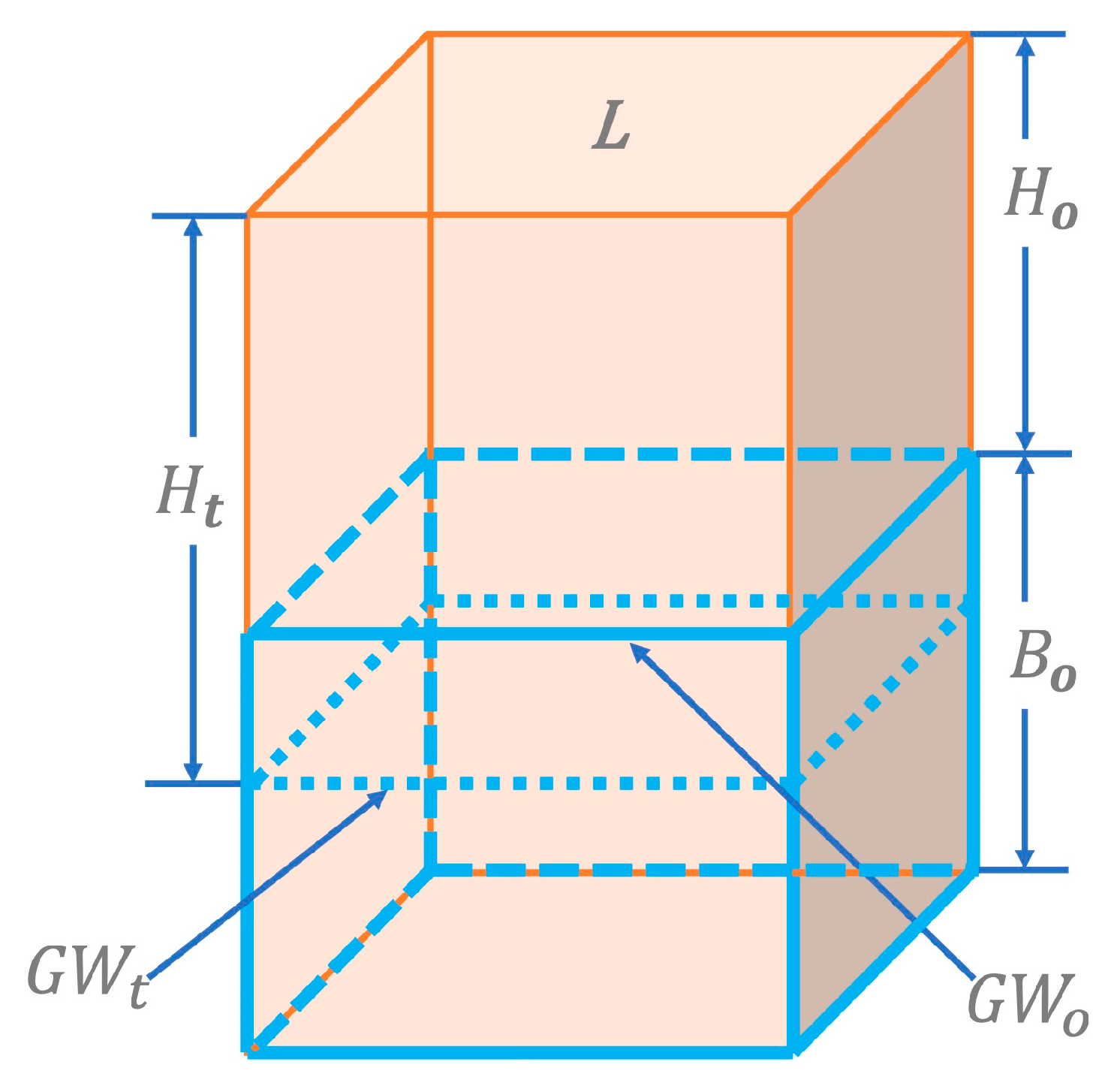
This paper simplifies those models to one perennial crop and one annual crop, with agronomic parameters based mostly on almonds and alfalfa, to relieve the computational burden of DP. Many other potential decisions, such as irrigation methods, urban water conservation, and water market decisions, are so far not included. These simplifications should not overly limit model application, as (i) the difference between perennial and annual crop profit is often large, so overall crop decisions change little when considering additional annual crops; (ii) agriculture is the predominant water user in San Joaquin Valley, with lower unit economic value than urban use; and (iii) higher efficiency irrigation methods appear more often in more arid regions. This paper’s model expands earlier models to include variable rather than constant pumping costs according to initial and final groundwater storage GWt−1 and GWt (which can be converted to groundwater levels (Figure 2)), to study overdraft management, and more explicit examination of results across dry to wet water years.
The decision variables are perennial crop acreage X p , t , annual crop acreage X a , j , t , pumping volume W p , j , t , and land for artificial recharge X r , j , t in WYT j and current decade t (i.e., the length of planning horizon T = 10 to represent that perennial crop acreage cannot change easily in the planning decade with WYTs).
The objective is to maximize the total net expected benefits Z t in decade t (Equation (1) with detailed derivations in Appendix A), which comes from decisions made in two stages. In the first stage, the benefit includes the total net benefits of perennial crops collected in decade t, B 1 t (Equation (A1)), and the initial perennial crop establishment cost only occurs in the first year, I N I P t (Equation (A2)). In the second stage, each year can be any possible WYT j with a probability of p j and amounts of surface water available s w j . These hydrologic probabilities do not yet vary with time t in this paper, which would add computational burden to the dynamic program. Each possible WYT j in the second stage can have different decisions for annual crop acreage X a , j , t , aquifer recharge X r , j , t , and pumping W p , j , t , resulting in different net benefits of annual crops and water operating costs. The temporary change in perennial crop acreage is not considered in the second stage because perennial crops are costly to abandon once planted due to high establishment and removal costs. Therefore, the model’s second stage derives the expected net annual crop return, B 2 t (Equation (A3)) less the expected conjunctive water operation cost, E X P C t   (Equation (A4)) that includes the cost of surface water, artificial recharge (a function of X r , j , t ), and pumping W p , j , t (a function of initial and final groundwater storage G W t 1 and G W t ). Any pumping fee to regulate overpumping is not included in this model but can be partially explored using the Lagrange multipliers on groundwater target constraints.
max Z t = B 1 t X p , t I N I P t X p , t , X p , t 1 + B 2 t X a , j , t E X P C t X r , j , t , W p , j , t , G W t 1 , G W t
The objective function (Equation (1)) is limited by land availability (Equation (2)), surface water availability (Equation (3)), and an expected groundwater mass balance constraint (Equation (4)).
Equation (2) constrains the acreage of perennial crops and annual crops, plus the area for artificial recharge to not exceed the total land available L (Figure 2) for each WYT j and decade t.
L X p , t X a , j , t X r , j , t   0   j
Equation (3) represents the water balance constraint for each WYT j and decade t. The water used to irrigate perennial and annual crops (assuming crops per unit area water consumption to be constant throughout all WYTs) and to recharge should not exceed the available surface water and pumped groundwater. aw is the annual applied water on the crop, and cap is the yearly recharge capacity per unit area.
s w j + W p , j , t c a p × X r , j , t a w p X p , t a w a X a , j , t 0   j
A single irrigation efficiency factor φ is used for simplicity to represent the portion of applied water percolating to the underlying aquifer. So Equation (4) calculates the expected mass balance of groundwater storage for decade t : the aquifer has a groundwater volume of G W t 1 at decade t , receiving the expected total deep percolation (sum of the deep percolation over a decade from the perennial crop, T φ a w p X p , t , and annual crop, T j = 1 5 p j φ a w a X a , j , t ), and the expected artificial recharge over the decade, T j = 1 5 p j c a p X r , j , t (assume all recharged water reaches the aquifer with no water lost in the vadose zone), and extracted an expected amount of groundwater over T years, T j = 1 5 p j W p , j , t , leads to the final groundwater storage of decade t , G W t . Yao [49] provides more discussion on this stochastic groundwater mass balance constraint.
G W t = G W t 1 + T φ a w p X p , t + T j = 1 5 p j φ a w a X a , j , t + T j = 1 5 p j c a p X r , j , t T j = 1 5 p j W p , j , t

2.2. Outer Model Formulation

Previous studies often use DP with two modules to derive intra- and inter-seasonal optimal water allocation policy [39,50,51,52]. The first inner module is an intra-seasonal model to make decisions maximizing crop net benefits given seasonal inputs such as the initial and final reservoir storage. The second outer module uses DP to find optimal seasonal decisions (as input conditions of the inner module) to maximize the total economic performance of the entire planning horizon.
This paper extends the two-module approach to decadal and century time scales (for groundwater systems with sufficient within-year seasonal storage). The first module, having the same objective function as the inner model described above, maximizes net benefit within decade t, including economically optimal conjunctive water use operations (land for recharging and groundwater pumped) and annual crop acreage, given the boundary conditions of initial and final groundwater storages/levels of decade t, and perennial crop acreage at the beginning of decade t before and after new perennials are planted.
The second outer module here is a DP that maximizes long-term discounted net benefits with decision variables for the initial and final groundwater storages/levels of decade t, and perennial crop acreage before and after new perennials are planted in decade t. These decisions become boundary conditions for the inner models run within the DP. For each combination of final groundwater storage and total (incoming plus newly planted) perennial crop acreage, the inner model calculates the optimal benefit of decade t (with decisions of land for recharging, groundwater pumped, and annual crop acreage). Then, the best combination of each decade is chosen, which can yield the highest sum of expected net discounted benefits of this decade and all later decades, given the initial groundwater storage and incoming perennial crop acreage.
The long-term planning horizon has N + 1 planning decades (from decade t = 0 to N, N = 9). A fixed inflation-adjusted discount rate r converts future values to present value. For each decade t, initial groundwater storage G W t 1 and incoming perennial crop acreage X p ,   t 1 are two state variables, while the expected final groundwater storage G W t (Equation (4)) and total (incoming plus newly planted) perennial crop acreage at the beginning of decade t, X p ,   t , are the two decision variables. The final groundwater storage of decade t , G W t , is also the initial groundwater storage of decade t + 1, while half of the perennial crops were retired (i.e., X p ,   t = 1 2 X p ,   t ). This provides a simple relationship from a decision variable in the current decade to a state variable in the next decade. Assuming that perennial crop acreage is maintained as high as possible for almost all decades to achieve the highest possible profit, a 50% retirement rate means that most perennial crops can stay productive for 20 years, roughly almond trees’ production life. For example, 75,000 acres of perennial crops from decade t enter decade t + 1, in which another 75,000 acres of perennial crops are newly planted (the maximal perennial crop acreage is fixed to be 150,000 acres). A 50% retirement rate means the 75,000 acres of perennial crops planted in decade t are to be retired before entering decade t + 2, and these 75,000 acres of perennial crops have been productive over decades t and t + 1 (i.e., 20 years). A limitation of this assumption is that if perennial crop acreage decreases, a 50% retirement rate can result in some perennial crops being productive for 30 years, which might exceed normal perennial crop productivity.
An objective function for the inner model describes the economic consequence of decisions and states. Let Π t G W t 1 ,   X p , t 1 , G W t , X p , t be the expected net present economic value of having groundwater storage from G W t 1 to G W t , and planting new perennial crop acreage of X p , t X p , t 1 . The overall objective is to maximize the sum of the expected net present value of profit from decade t = 0 to N:
M a x   t = 0 N Π t G W t 1 ,   X p , t 1 , G W t , X p , t  
The equivalent backward recursive function is as follows:
f t G W t 1 , X p , t 1 , G W t , X p , t = Π N G W N 1 , X p , N 1 , G W N , X p , N ,   t = N Π t G W t 1 , X p , t 1 , G W t , X p , t + f t + 1 * G W t , X p , t = 1 2 X p , t ,   t = 0   : N 1
In this approach, given a pre-specified final groundwater storage goal G W N , the optimal decision in t = N (i.e., the perennial crop acreage, X p , N ) is determined first to maximize Π N G W N 1 ,     X p , N 1 , G W N , X p , N as a function of two state variables: initial groundwater storage G W N 1 and incoming perennial crop acreage X p ,   N 1 . Next, the next-to-last decade’s ( t = N 1 ) optimization involves maximizing the sum of decade N 1 ’s decade-specific objective function Π t G W t 1 ,   X p , t 1 , G W t , X p , t and the optimal value of the future objective function f t + 1 * G W t ,   X p , t = 1 2 X p , t , giving that decade’s optimal decisions contingent upon the value of the state variables as of the next-to-last-decade decision. This logic continues recursively back in time, until the first decade decision is determined. f t + 1 * G W t ,   X p , t is the accumulated present economic value of the best decisions from all later decades, starting with groundwater storage G W t and incoming perennial crop acreage of X p , t .
The difference between Π t (Equation (7)) and Equation (1) is that in Π t , the perennial crop acreage is input from the outer DP model as X p , t instead of being derived to maximize profit in only one decade. Π p , t , Π a , t , and C t in Equation (7) are the equivalent to B 1 t I N I P t , B 2 t , and E X P C t in Equation (1), respectively. Π t still needs to be maximized in each decade t to derive the optimal decision of annual crop acreage ( X a , j , t ) and conjunctive water management (land for recharging X r , j , t and the amount of pumping W p , j , t ) in decade t with j possible WYTs, given the initial and final groundwater storage, G W t 1 and G W t , incoming perennial crop acreage, X p , t 1 , and total perennial crop acreage before retirement, X p , t .
max   Π t G W t 1 ,   X p , t 1 , G W t ,   X p , t = Π p , t X p , t 1 , X p , t + Π a , t X a , j , t C t X r , j , t , W p , j , t , G W t 1 , G W t

2.3. Model Assumptions and Limitations

Several underlying assumptions are worth discussing. All modeling requires simplifications. First, here, the aquifer is treated as a closed homogeneous box with no drainage to other streams and basins, and no other means to replenish except for recharge basins and deep percolation from applied irrigation water (assuming all the recharge water reaches the water table without water loss in the vadose zone). Recharge from precipitation is not included. This simplifies many real-world situations. Also, since the inner model is not a seasonal model but a 10-year model, on-farm recharge in winter is not considered explicitly, and aquifer recharge uses different lands with annual crops. The surface water can only be used for either aquifer recharge or crop irrigation, meaning if surface water is allocated to aquifer recharge, at least some crops will not be grown. Moreover, since only recharge from percolation is considered, recharge to the confined aquifer is omitted in the study. However, in some areas, a confined aquifer is the production layer.
Second, groundwater storage is assumed to be enough so the Lagrange multiplier for groundwater in sensitivity analysis is constant across decadal WYTs, that the change in groundwater depth in a decade is not large and unit pumping cost is constant within each decade, and that water pumped and recharged does not affect groundwater availability for irrigation within a decade. Furthermore, the final groundwater storage of each decade in the DP is an expected value rather than an exact one, which might overestimate or underestimate total profit. And surface water hydrology is assumed to be stationary.
This study could also be improved to include soil water contributions to seasonal crop water use, impacts of deficit irrigation and salinity in groundwater and soil on crop yield, and more different crops with their particular evapotranspiration. Different irrigation methods and dual irrigation systems also can be considered. Furthermore, this paper assumes irrigation demands for crops do not change across WYTs and climate scenarios. Additionally, perennial crops are sensitive to chill hours, and frost and freezing, which could be considered in future studies, necessitating a bigger model. More detailed modeling of perennial crops would be useful for future studies. That half of perennial crops are retired (without including costs) before entering the next decade instead of annually retiring 5% of perennial crops overestimates the establishment cost as all newly planted perennials are planted in the first year of the decade, which is discounted least. On the other hand, this model assumes perennial crops fruit in the first year, and productivity does not vary as orchards age, which overestimates perennial crops’ profit.
Finally, this model does not include groundwater quality, mitigation of land subsidence, and increased interaction between surface water for environmental purposes, which left ample room for further research. Yao et al. [7] consider water quality effects, particularly groundwater salinity.

2.4. Case Example

Table 1 summarizes the parameters used in this example of agricultural area and underlying aquifer (Figure 2). This hypothetical basin is developed for model development and exploration, and not to represent any particular area, although it is broadly similar to parts of California’s SJV. For computational and illustrative reasons, two crops (are represented (Table A1) in Appendix A): a perennial crop (with parameters based on almonds) and an annual crop (with characteristics of alfalfa). Both firm contract water (for water allocated in most years) price c c l a s s 1 , and surplus water (for additional water available in wet years) price c c l a s s 2 are based on the Chowchilla water district, while actual surface water sources are more complex. The unit price of energy is adopted from the Statewide Agricultural Production (SWAP) model for North San Joaquin Valley [53]. For the decadal model, initial groundwater storage is 12.3 billion m3 (10 MAF) with 30,351 ha (75,000 acres) of incoming perennial crops. The century DP model has initial groundwater storages ranging from 9.87 to 14.8 billion m3 (8 to 12 MAF) with an interval of 617 million m3 (0.5 MAF) and incoming perennial crop acreages of 30,351 ha (75,000 acres) for the first decade, and a groundwater storage goal of 12.3 billion m3 (10 MAF). The discretization of two decision variables in outer DP is 617 million m3 (0.5 MAF) for groundwater storages and 4047 ha (10,000 acres) for perennial crop acreage, respectively.
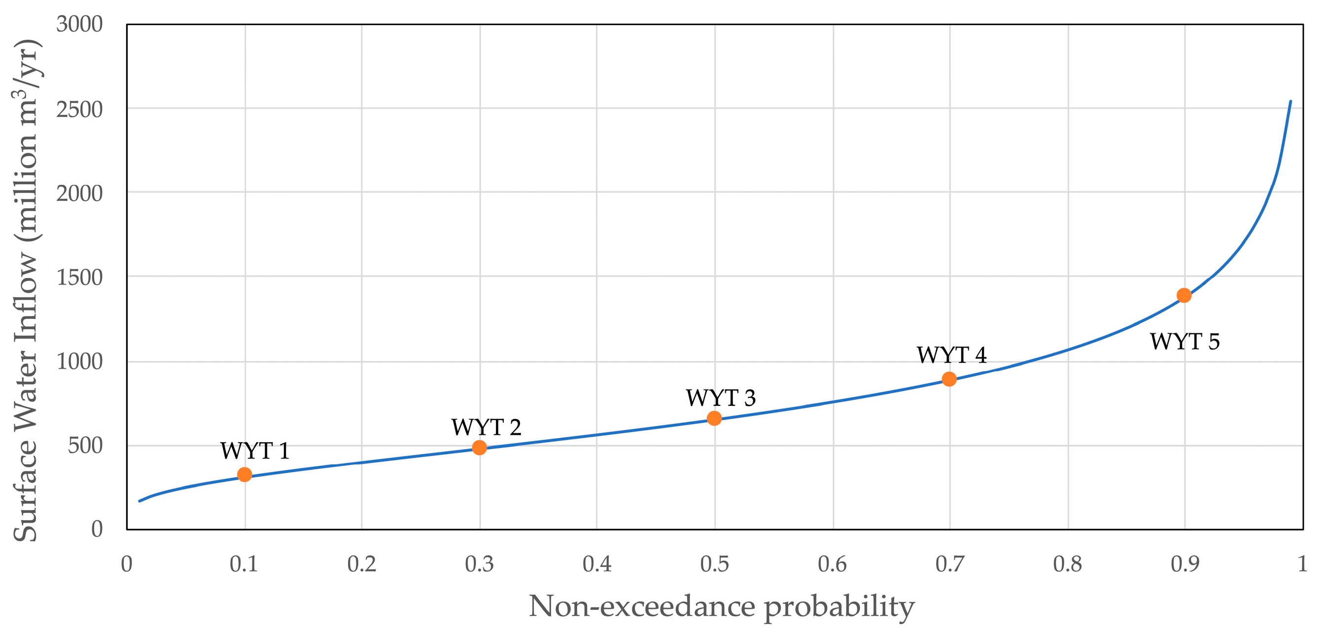
Table 2 and Figure 3 characterize the distribution of surface water availability s w ~ l o g N ( μ = 771 million m3 (625 thousand acre-ft (TAF)), σ = 493 million m3 (400 TAF) ) . For simplicity, each water year type’s (WYT’s) surface water inflow is represented by the 10th-, 30th-, 50th-, 70th- and 90th-percentile of the distribution, so that in the base case, all WYT has the same probability of occurrence, 20%. Given that the 617 million m3 of water is firm contracted (Table 1), there is a 40% chance that firm contract water is only partially supplied (Table 2), and surplus surface water is only available in WYTs 3 to 5.

3. Results

Integrated profit maximizing optimization across timescales suggests some economically promising strategies for perennial and annual cropping decisions and water management to balance groundwater resources. Optimal decadal timescale strategies (from the inner model) represent a near-term way to change groundwater storage, and outer model DP results suggest long-term strategies to stage the end of groundwater overdraft. Different discount rates and different climate scenarios are considered to see the effects of hydrologic and economic climates on crop mix and conjunctive water operations. Additional findings are available in Yao [49].

3.1. Conjunctive Use and Cropping for Within-decade Timescales

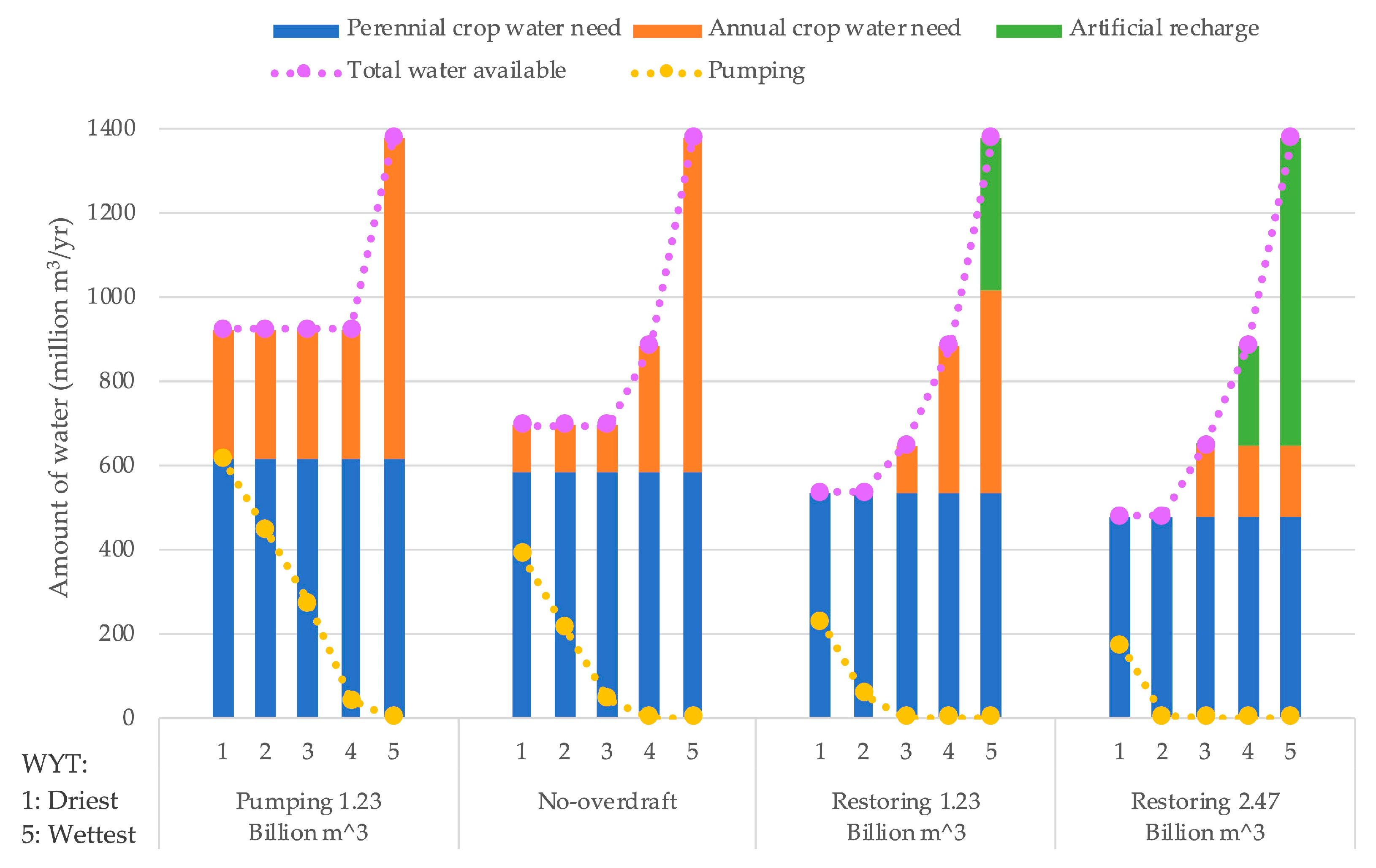
For the decadal model, initial groundwater storage is 12.3 billion m3 (10 MAF) with 30,351 ha (75,000 acres) of incoming perennial crops. Different recovery goals are explored, from net groundwater drawdown of 1.23 billion m3 (1 MAF) to net groundwater recovery of 2.47 billion m3 (2 MAF) within 10 years. Figure 4 shows that more groundwater is pumped in drier years to irrigate crops, some of which comes from the water artificially recharged in wetter years, often reducing wetter-year annual crop acreages. Conjunctive use of surface water and groundwater smooths the variable water availability to stabilize crop production and profitability across different water years. This is a common pattern for real conjunctive use systems.
Furthermore, perennial crops’ high initial establishment cost limits the growth of perennial crop acreage from 38,717 ha (95,671 acres) at net recharge of the aquifer of 2.47 billion m3 (2 MAF) to 49,483 ha (122,276 acres) at overall pumping of 1.23 billion m3 (1 MAF), with only an increase by 27%. For annual crops, the agricultural production model’s quadratic crop profit (see Equation (A3) in Appendix A) with diminishing marginal profit drives the model to have the same acreage in WYTs with pumping or artificial recharge to maximize expected net profit.
The Lagrange multipliers of the water constraints estimate the economic value of surface water and groundwater (Table 3). High groundwater storage capacity allows groundwater to have constant value across water years. These results show surface water is usually preferred to groundwater due to pumping costs and the value of irrigation (containing surface water) return flows contributing to groundwater recharge. However, adding capital costs for surface water infrastructure for storage, diversion, conveyance, and distribution could affect results. Other benefits from groundwater use reduction, such as land subsidence mitigation, less groundwater quality degradation, the increase in the interaction between surface streams and groundwater, and ecosystem restoration, are also omitted.
Surface water has a higher value in drier years because one unit less surface water in those years harms higher-value perennial crops rather than lower-value annual crops. Table 3 also shows that the value of surface water and groundwater decreases when aquifer restoration goals become more relaxed. Even though groundwater still has a positive value when 1.23 billion m3 (1 MAF) is pumped, indicating the most relaxed goal has the highest expected net profit, the marginal profit decreases with increased pumping and greater water availability. In other words, unlimited pumping does not always have the highest profit. Net pumping of 4.93 billion m3 (4 MAF) leads to a lower profit than a net pumping of 3.70 billion m3 (3 MAF).
All WYTs with pumping (values in bold) and all WYTs with artificial recharge (values in italics) each have the same economic value of surface water (Table 3) and the same acreage of annual crops (Figure 4). This confirms that optimal conjunctive water management moves water from wetter years to drier years to dampen variability in surface water availability, marginal value, and cropping.
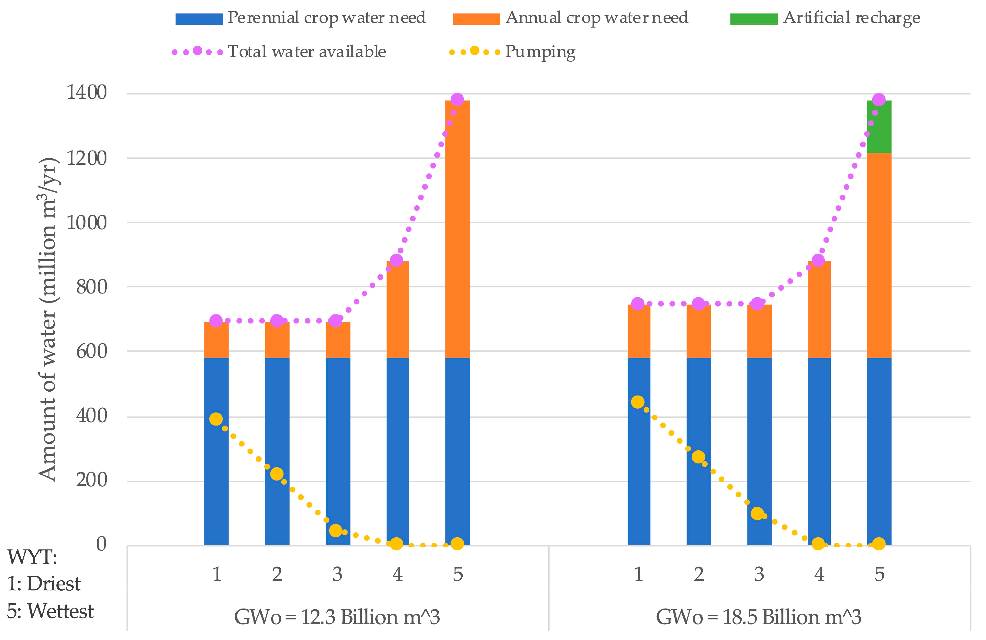
Higher initial groundwater storage/level can also change the optimal conjunctive water use and cropping pattern and increase profit with the same no-overdraft goal. From Table 4 and Figure 5, though the perennial crop’s high initial establishment cost prevents its acreage from growing, pumping is more encouraged in drier years when initial groundwater storage is higher as pumping energy cost is lower with the lower lift. More annual crops are grown in drier years when the marginal profit is higher (as the acreage is still lower than in wetter years). Savings in unit pumping cost and increased profit for more annual crops in drier years are strong enough to motivate artificial recharge with additional cost in the wettest year, displacing some annual crop acreage in these wetter years, which is not recommended when the initial groundwater storage/level is lower for the same change of groundwater storage.

3.2. Groundwater Management and Cropping for Long-Term Timescales

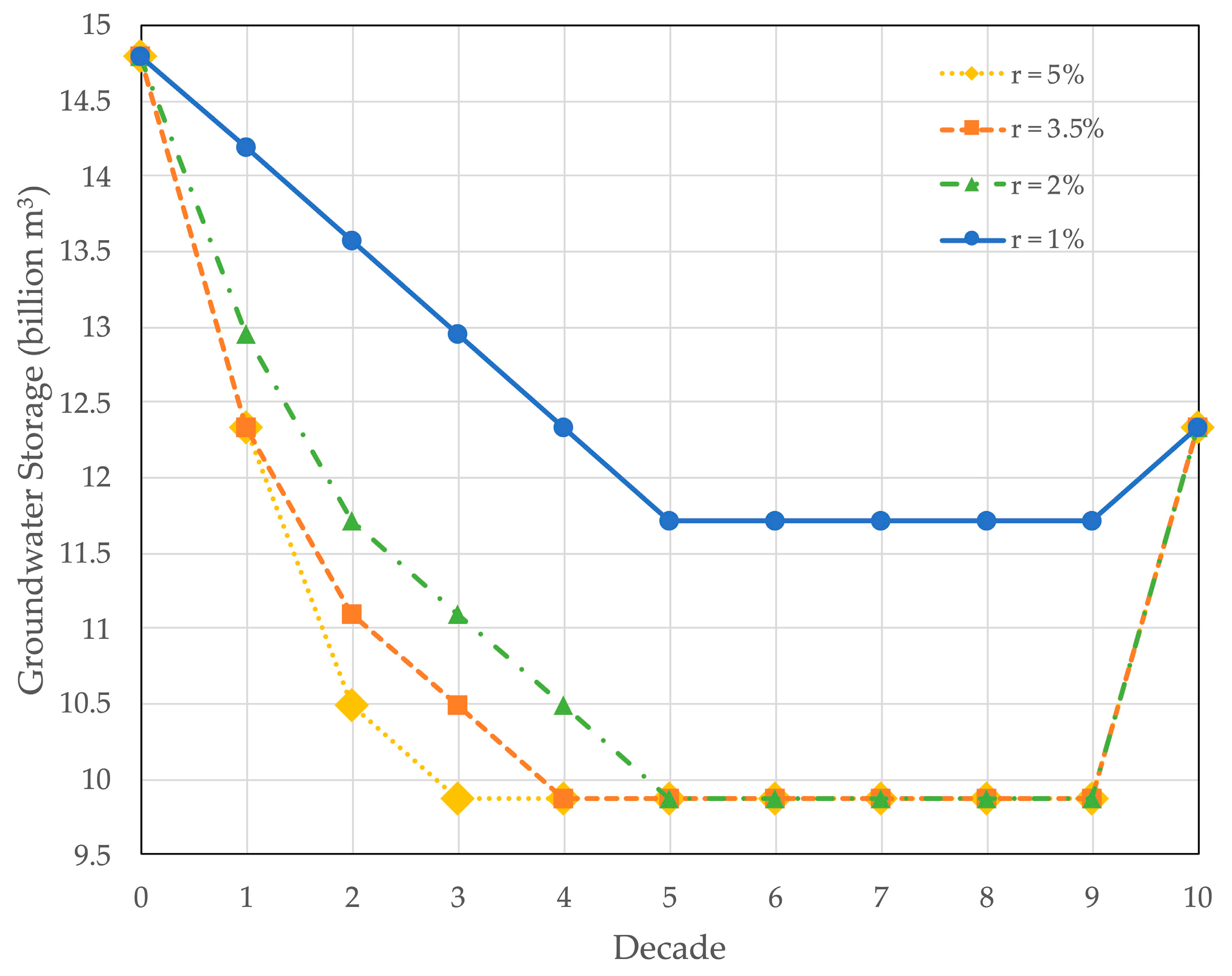
Economically optimized single-decade decisions change with longer-term timescale. Single-decade optimal decisions tend to be more aggressive in pumping to maximize profit, not knowing future decades also require enough pumping to maintain high profit. However, an optimal decade in the context of longer-term decisions must end groundwater overdraft at target groundwater levels (this paper examines a range of initial groundwater storages from 9.87 to 14.8 billion m3 (8 to 12 MAF) with a final groundwater storage goal of 12.3 billion m3 (10 MAF)). Long-term optimal solutions allocate groundwater pumping over decades. It is most profitable to pump more mildly while still maximizing higher-value perennial crop production until no further net drawdown is allowed (Figure 6); in other words, the minimum threshold defined in SGMA, and finally, recharge the aquifer to the groundwater storage target.
Figure 7 compares shorter-term optimal decisions considering only one decade and longer-term optimal decisions. When no overdraft is allowed, compared to the decadal model decisions, the longer-term optimization has more perennial crops (shown as higher blue columns in Figure 7a). Moreover, when net pumping is allowed, the decadal model suggests pumping 3.7 billion m3 (3 MAF) to have the highest expected net profit, while the first decade of longer-term optimization only pumps 2.47 billion m3 (2 MAF) (as yellow markers in Figure 7b for decadal optimal decisions are never less than long-term decisions) so later decades can also pump groundwater with lower unit pumping cost to preserve future profit. But even with pumping 1.23 billion m3 (1 MAF) less than the decadal optimum, the first decade in the long-term optimum grows more perennial crops to reduce the planting cost of perennial crops in later decades. This reflects what is happening in California, where more perennial crops are grown to increase profits, and even water becomes scarcer. However, this is only possible by paying more for additional pumping in drier years and additional artificial recharge and reduced pumping in wetter years, with fewer annual crops overall.

3.3. Sensitivity Analyses

3.3.1. Different Discount Rates

For (semi)arid irrigated regions similar to California’s San Joaquin Valley, neglecting salinity considerations, economically optimal management increases drawdown initially and delays groundwater storage recovery until the final decade to meet the sustainability target (Figure 6). Both the depth and speed of drawdown and the magnitude of aquifer recharge increase with higher discount rates, which give greater weight to near-term benefits relative to more distant costs.
Higher discount rates reduce perennial crop planting in single-decade decisions because the high establishment costs of perennial crops in the first year are substantial compared to benefits in later years. However, to save planting costs for perennial crops in future decades, perennial crop acreage is not affected by discount rates except in the later recovery decades (Yao [49] has more detailed discussion).

3.3.2. Climate Effects

This sensitivity analysis increases WYT 1 and 2’s probability of occurrence to create drier and even drier scenarios, therefore wetter WYTs become more unlikely (Table 5).
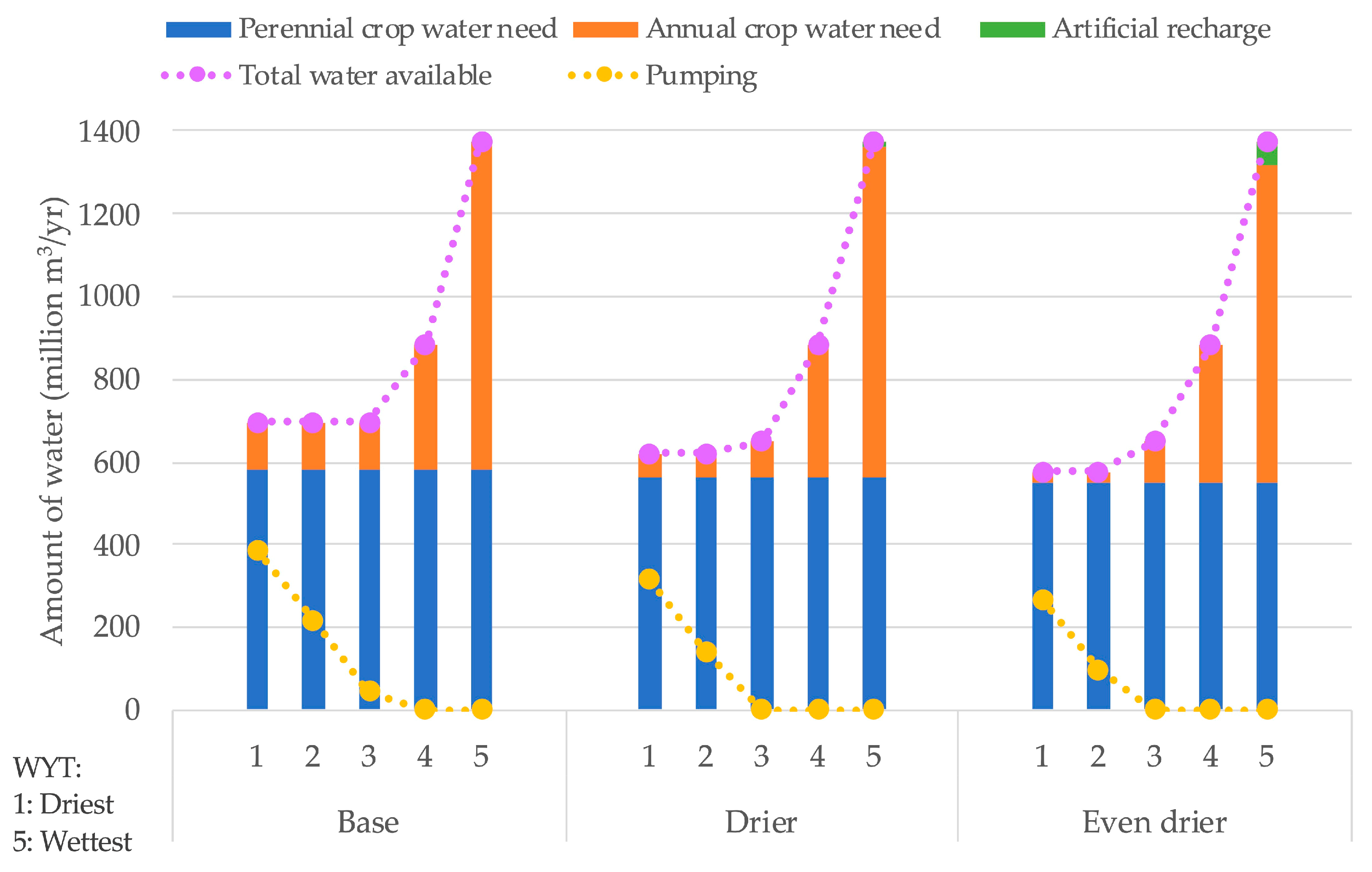
Figure 8 and Table 6 show differences in cropping and pumping decisions for three climate scenarios with no net change in groundwater storage for a decadal timescale. The model suggests less pumping in drier years with drier climates overall and lower expected pumping for the entire decade. This is accomplished by decreasing perennial crop acreage across the decade and further reducing annual crops in drier years. The costs for pumping in more frequent drier years and more artificial recharge in wetter years (to offset the increased pumping) make maintaining the same acreage of perennial and annual crops in drier years less economical (as the summed height of orange and blue columns are lower in drier WYTs with drier climates).
Artificial recharge is not greatly expanded even for drier climates (shown as short green columns in Figure 8 and only a small area for artificial recharge in Table 6). This underscores the expense of artificial recharge to stop groundwater overdraft relative to opportunity costs of more annual crops in wet years. From Figure 6, where artificial recharge occurs only in the last stage, aquifer recovery is not performed voluntarily nor smoothly if the groundwater management is purely driven by profit maximization without a regulatory framework such as pumping restrictions or taxes from water agencies unless other factors restrict crop yield and profit (e.g., groundwater salinity [7]).
For the isolated 10-year optimization, drier climates reduce profit and increase the value of groundwater due to surface water scarcity (Table 7). Drier climates increase the economic value of surface water in dry years because perennial crops are more likely to be harmed by water scarcity. But surface water’s economic value drops in wetter years, as perennial crops become a smaller proportion of crops planted, and annual crops are the first crops fallowed when surface water is under shortage. The value of surface water in the wettest WYT in the even drier climates is slightly higher than in drier climates because less surface water in that WYT means less artificial recharge, which impairs perennial crops and perhaps slightly increases pumping costs in drier years.
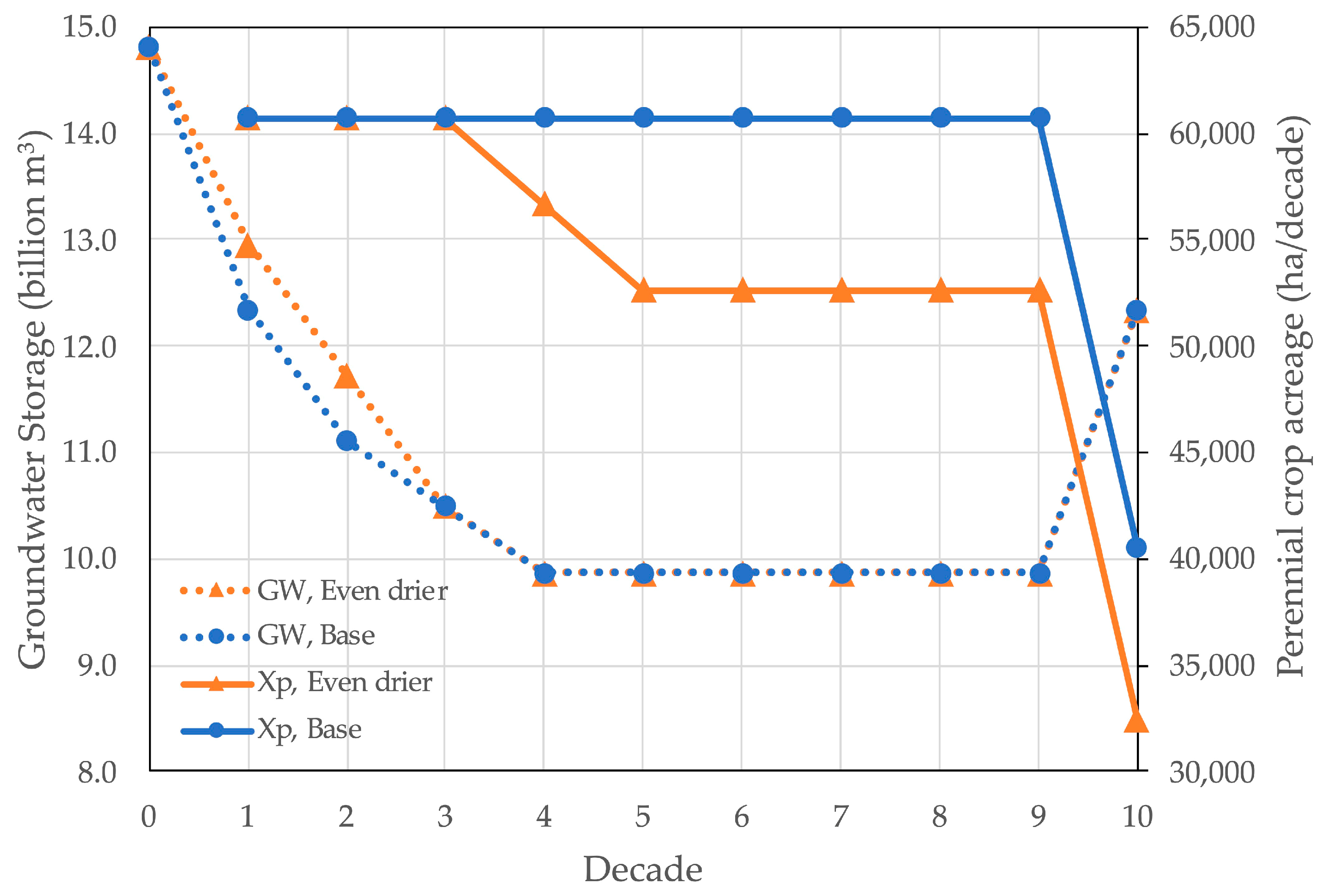
For the base climate, keeping no overdraft can still maintain perennial crop acreage at maximum (Figure 9), with some artificial recharge in the wettest years (Figure 7a), to save the planting cost of perennial crops in the next decade while maintaining an acceptable profit in the current decade. Discounting drives more pumping in the early decades (Figure 6) because the revenue of growing annual crops exceeds the additional pumping cost.
For the even drier climate, a net pumping of 1.23 billion m3 (1 MAF) is needed to maximize perennial crop acreage. And because higher profit requires more perennial crops in the early decades, which are less discounted, it is not economical to pump too much groundwater in the first decades for annual crops. So, drier climates reduce overall pumping in the early decades for the long-term timescale (Figure 9).
In the even drier climate, fewer annual crops are grown, so groundwater pumping is reduced in the first decade from the base climate, allowing decades 2 and 3 to maintain the maximum acreage of perennial crops (Figure 9). To understand pumping reduction in the first decade for the even drier climate, it is needed to compare the saved planting cost of perennial crops in later decades (which are more discounted) and the decreased profit from annual crops in earlier decades. The DP model only reduces pumping in decade 1 by 617 million m3 (0.5 MAF) instead of 1.23 billion m3 (1 MAF) in the base climate to keep some annual crops at the cost that decade 4 must begin reductions in perennial crops acreage. So, the model recommends using groundwater as much and as soon as possible until it starts to impact later perennial crop production.
In a long-term timescale, climate and initial groundwater availability do have an impact on the economic value of surface water. A much drier climate increases the marginal economic value of surface water for agriculture by about 30 cents per cubic meter or several hundred dollars per acre-foot (Table 8). Lower groundwater availability further amplifies the importance of surface water. A drier climate also increases the value of groundwater, but not as much as the effect on surface water (Table 7 and Table 9).

4. Conclusions

Groundwater often serves as an inter-annual reservoir for drier years, sustaining more profitable perennial crops through drought. Perennial crops’ generally higher net returns and initial establishment cost may drive farmers to increase or keep irrigated areas of perennial crops, which makes water management less flexible and more costly because of more pumping in drier years and more artificial recharge or reduced annual crops in wetter years, as unlimited pumping does not always lead to the highest profit. Farmer’s profit maximization can predict reductions in annual crop acreage because pumping in drier years to grow annual crops is less profitable and artificial recharge reduces water available to irrigate annual crops even in non-dry years.
Due to their costs, artificial recharge and aquifer recovery are often less common for profit-maximizing farmers. Economic discounting over time, which increases near-term benefits and costs relative to those in the more distant future, tends to exacerbate the drawdown. Even when given 100 years to restore groundwater storage, recovery operations tend not to begin until late in the planning horizon. Regarding climate change, drier climates reduce profit by limiting the acreage of perennial crops and decreasing expected pumping across a decade, which increases the range of surface water prices and average water prices.
This work assesses the economic value of conjunctively managed water for irrigated agriculture over varying climatic and economic conditions under decadal and century timescales. It has found some fundamental economic tendencies in the long-term economics driving conjunctive use over short and long timescales. The approach also identifies promising cropping patterns for meeting groundwater sustainability objectives while maintaining overall agriculture economic viability.
Such analyses unavoidably simplify actual conditions, providing some general insights but leaving room for more detailed research and applications. Further studies could improve groundwater physics representation, reflect more farming reality, especially under climate change, demand management such as administrative pumping fees, and quantitative evaluation of additional benefits of ending overdraft, such as reducing land subsidence, improving groundwater quality, and ecosystem restoration.

Author Contributions

Conceptualization, Y.Y. and J.R.L.; methodology, Y.Y., J.R.L. and J.M.-A.; formal analysis, Y.Y. and J.R.L.; writing—original draft preparation, Y.Y.; writing—review and editing, Y.Y., J.R.L. and J.M.-A.; visualization, Y.Y.; supervision, J.R.L.; funding acquisition, J.R.L. All authors have read and agreed to the published version of the manuscript.

Funding

This research was partially funded by the US-China Clean Energy Research Center for Water-Energy Technologies (CERC-WET), grant number #DE-1A0000018. Any opinions, findings, conclusions, or recommendations expressed in this paper are those of the authors and do not necessarily reflect the views of funders.

Data Availability Statement

Datasets for this research are preserved by the internet archive: https://web.archive.org/web/20170711215918, https://water.ca.gov/economics/downloads/Models/SWAP_TechAppendix_080612_Draft.pdf (accessed on 27 March 2024). These datasets, coupled with model formulation and results, are also available at https://doi.org/10.5281/zenodo.5889557 (accessed on 27 March 2024) and https://github.com/YiqingYao/Conjunctive_w_Perennials (accessed on 27 March 2024).

Acknowledgments

The authors are thankful to Jonathan Herman, Samuel Sandoval Solis, Lucia Levers, and anonymous reviewers for comments and proofreading that helped improve the paper.

Conflicts of Interest

The authors declare no conflicts of interest.

Appendix A

Table A1 provides parameters of baseline annual agricultural production adopted from the SWAP model for North San Joaquin Valley [53] and a quadratic cost function obtained through Positive Mathematical Programming (PMP) [31]. PMP is a self-calibrating method that captures non-linearities in cropping decisions with exact calibration to a baseline production dataset [31]. In this application, a quadratic cost function is employed; hence, a linear marginal cost function with intercept parameter α and slope parameter γ (Table A1) for two crops was estimated by following the methods available at: https://doi.org/10.5281/zenodo.5889557 (accessed on 22 April 2024) and https://github.com/YiqingYao/Conjunctive_w_Perennials (accessed on 22 April 2024).
The total net expected benefits in decade t , Z t (Equation (1)), can be further derived. B 1 t (Equation (A1)) is the sum of discounted profits of perennial crops over a decade ( T = 10). The perennial crop acreage over the decade is always X p , t , so B 1 is a sum of geometric series. v p and y l d p (Table A1) are the unit price and yield of perennial crops and α p and γ p (Table A1) are the PMP intercept and slope parameters of perennial crops. r is the constant discount rate (Table 1).
B 1 t ( X p , t ) = v p y l d p X p , t α p + 1 2 γ p X p , t X p , t ÷ ( 1 + r ) t T + 1 + v p y l d p X p , t α p + 1 2 γ p X p , t X p , t ÷ ( 1 + r ) t T + 2 + + v p y l d p X p , t α p + 1 2 γ p X p , t X p , t ÷ ( 1 + r ) t T + 10 = v p y l d p X p , t α p + 1 2 γ p X p , t X p , t 1 1 + r T ( 1 + r ) t T × r
Table A1. Base year (in 2005 dollars) observations and estimated PMP production cost functions.
Parameter (Unit)Perennial Crop
(Similar to Almonds)
Annual Crop
(Similar to Alfalfa)
Base year
observations
Area   X ~ (ha)132,87467,724
Yield   y l d (kg/ha) 224217,934
Price   v ($/kg)4.660.173
Applied   water   a w   (m/ha)3.073.65
Land cost ($/ha)2006783
Other supply cost ($/ha)41461344
Labor cost ($/ha)78652
Total cost ($/ha)69392179
PMP cost function Intercept   α ($/ha)3713.621571.37
Slope   γ ($/ha2)0.04850.0180
The perennial crop establishment cost, I N I P t , is determined by the initial acreage of perennial crops in the current decade, X p , t , and the incoming perennial crop acreage, X p , t 1 . If new perennial crops are to be planted, i.e., X p , t > X p , t 1 , the establishment cost is the acreage of newly planted perennial crop times the unit price of establishment cost, i n i p (Table 1), multiplied by the discount factor. Otherwise, there is no establishment cost (Equation (A2)).
I N I P t X p , t , X p , t 1 = max X p , t X p , t 1 , 0 i n i p ÷ ( 1 + r ) t T + 1
The expected net benefit of planting annual crops over a decade ( T = 10), B 2 t (Equation (A3)), is the sum of the present value of annual expected net benefits, which is the weighted average of annual crop profit in WYT j with the probability of p j . v a and y l d a (Table A1) are the unit price and yield of annual crops and α a and γ a (Table A1) are the PMP intercept and slope parameters of annual crops. Because the hydrology is stationary, in other words, p j is constant for all j , Equation (A3) is a sum of geometric series.
B 2 t X a , j , t = 1 ( 1 + r ) t T + 1 j = 1 5 p j v a y l d a X a , j , t α a + 1 2 γ a X a , j , t X a , j , t + 1 ( 1 + r ) t T + 2 j = 1 5 p j v a y l d a X a , j , t α a + 1 2 γ a X a , j , t X a , j , t + + 1 ( 1 + r ) t T + 10 j = 1 5 p j v a y l d a X a , j , t α a + 1 2 γ a X a , j , t X a , j , t = 1 1 + r T ( 1 + r ) t T × r j = 1 5 p j v a y l d a X a , j , t α a + 1 2 γ a X a , j , t X a , j , t
E X P C t is the expected water operational cost over a decade ( T = 10). Similar to B 2 t , due to the stationary hydrology, it is also a sum of a geometric series of discounted yearly expected net water operational cost, which is the weighted average of annual water operational cost in WYT j with the probability of p j . Annual water operational cost is composed of pumping cost ( C p u m p · W p , j ), the cost of artificial recharge ( c l a n d · X r , j ), as well as the cost of firm contract and surplus surface water, where c l a n d is the unit price of land for recharging, c c l a s s 1 is the unit price of firm contract water and c c l a s s 2 is the unit price of surplus surface water (Table 1). In some WYTs, the surface water inflow s w j is even less than the c l a s s 1 or firm contract water, and c c l a s s 2 can only be applied to the remaining surface water, so the cost of firm contract and surplus surface water is calculated as c c l a s s 1 · min s w j , c l a s s 1 and c c l a s s 2 · max s w j c l a s s 1 , 0 , respectively.
E X P C t X r , j , t , W p , j , t , G W t 1 , G W t = 1 1 + r T 1 + r t T × r j = 1 5 p j C p u m p · W p , j , t + c l a n d · X r , j , t + c c l a s s 1 · min s w j , c l a s s 1 + c c l a s s 2 · max s w j c l a s s 1,0
Pumping cost is the product of the unit price of energy c e (Table 1) and total energy for pumping, which is a function of the amount of pumping, W p , j , t , and groundwater storage, as more energy is needed to pump from aquifers of lower storage (Figure 2). Therefore, the pumping cost ( C p u m p · W p , j , t ) in Equation (A4) expands to the following:
C p u m p · W p , j , t = c e [ $ k W h ] × W p , j , t [ m 3 ] × H [ m ] × ρ [ k g m 3 ] × g [ m s 2 ] 3.6 × 10 6 [ k W h J ] × η p
where H (Equation (A6)) is the average of the initial and final head (Figure 2), and η p is the pumping efficiency.
H = 1 2 H t 1 + H t = 1 2 H o + G W o G W t 1 L · s y + H o + G W o G W t L · s y = H o + 1 2 L · s y 2 G W o G W t 1 G W t                                                                   = H o + B o 1 2 L · s y G W t 1 + G W t                                                                              

References

  1. Reilly, T.E.; Dennehy, K.F.; Alley, W.M.; Cunningham, W.L. Ground-Water Availability in the United States; Geological Survey (US): Reston, VA, USA, 2008; ISBN 1-4113-2183-9.
  2. Faunt, C. Groundwater Availability of the Central Valley Aquifer. U.S. Geol. Surv. Prof. Pap. 2009, 1766, 225. [Google Scholar]
  3. Lund, J.; Medellin-Azuara, J.; Durand, J.; Stone, K. Lessons from California’s 2012–2016 Drought. J. Water Resour. Plann. Manag. 2018, 144, 04018067. [Google Scholar] [CrossRef]
  4. Escriva-Bou, A.; Hui, R.; Maples, S.; Medellín-Azuara, J.; Harter, T.; Lund, J.R. Planning for Groundwater Sustainability Accounting for Uncertainty and Costs: An Application to California’s Central Valley. J. Environ. Manag. 2020, 264, 110426. [Google Scholar] [CrossRef] [PubMed]
  5. Chen, X.; Hu, Q. Groundwater Influences on Soil Moisture and Surface Evaporation. J. Hydrol. 2004, 297, 285–300. [Google Scholar] [CrossRef]
  6. Pauloo, R.A.; Fogg, G.E.; Guo, Z.; Harter, T. Anthropogenic Basin Closure and Groundwater Salinization (ABCSAL). J. Hydrol. 2021, 593, 125787. [Google Scholar] [CrossRef]
  7. Yao, Y.; Lund, J.R.; Harter, T. Conjunctive Water Management for Agriculture with Groundwater Salinity. Water Resour. Res. 2022, 58, e2021WR031058. [Google Scholar] [CrossRef]
  8. Romero, E. Friant-Kern Canal Slows By 60 Percent, Subsidence To Blame. Available online: https://www.kvpr.org/environment/2017-08-03/friant-kern-canal-slows-by-60-percent-subsidence-to-blame (accessed on 22 April 2024).
  9. California Department of Water Resources California Aqueduct Subsidence Study. Available online: https://cawaterlibrary.net/wp-content/uploads/2017/11/Aqueduct_Subsidence_Study-FINAL-2017.pdf (accessed on 22 April 2024).
  10. Harou, J.J.; Lund, J.R. Ending Groundwater Overdraft in Hydrologic-Economic Systems. Hydrogeol. J. 2008, 16, 1039. [Google Scholar] [CrossRef]
  11. Dogan, M.S.; Buck, I.; Medellin-Azuara, J.; Lund, J.R. Statewide Effects of Ending Long-Term Groundwater Overdraft in California. J. Water Resour. Plan. Manag. 2019, 145, 04019035. [Google Scholar] [CrossRef]
  12. Alam, S.; Gebremichael, M.; Li, R.; Dozier, J.; Lettenmaier, D.P. Can Managed Aquifer Recharge Mitigate the Groundwater Overdraft in California’s Central Valley? Water Resour. Res. 2020, 56, e2020WR027244. [Google Scholar] [CrossRef]
  13. Buras, N. Conjunctive Operation of Dams and Aquifers. J. Hydraul. Div. 1963, 89, 111–131. [Google Scholar] [CrossRef]
  14. Burt, O.R. The Economics of Conjunctive Use of Ground and Surface Water. Hilg 1964, 36, 31–111. [Google Scholar] [CrossRef]
  15. Burt, O.R. Economic Control of Groundwater Reserves. Am. J. Agric. Econ. 1966, 48, 632–647. [Google Scholar] [CrossRef]
  16. Bredehoeft, J.D.; Young, R.A. Conjunctive Use of Groundwater and Surface Water for Irrigated Agriculture: Risk Aversion. Water Resour. Res. 1983, 19, 1111–1121. [Google Scholar] [CrossRef]
  17. Fredericks, J.W.; Labadie, J.W.; Altenhofen, J.M. Decision Support System for Conjunctive Stream-Aquifer Management. J. Water Resour. Plan. Manag. 1998, 124, 69–78. [Google Scholar] [CrossRef]
  18. Pulido-Velázquez, M.; Andreu, J.; Sahuquillo, A. Economic Optimization of Conjunctive Use of Surface Water and Groundwater at the Basin Scale. J. Water Resour. Plan. Manag. 2006, 132, 454–467. [Google Scholar] [CrossRef]
  19. Gorelick, S.M. A Review of Distributed Parameter Groundwater Management Modeling Methods. Water Resour. Res. 1983, 19, 305–319. [Google Scholar] [CrossRef]
  20. Bazargan-Lari, M.R.; Kerachian, R.; Mansoori, A. A Conflict-Resolution Model for the Conjunctive Use of Surface and Groundwater Resources That Considers Water-Quality Issues: A Case Study. Environ. Manag. 2009, 43, 470–482. [Google Scholar] [CrossRef]
  21. Tabari, M.M.R.; Soltani, J. Multi-Objective Optimal Model for Conjunctive Use Management Using SGAs and NSGA-II Models. Water Resour. Manag. 2013, 27, 37–53. [Google Scholar] [CrossRef]
  22. Naghdi, S.; Bozorg-Haddad, O.; Khorsandi, M.; Chu, X. Multi-Objective Optimization for Allocation of Surface Water and Groundwater Resources. Sci. Total Environ. 2021, 776, 146026. [Google Scholar] [CrossRef]
  23. Varela-Ortega, C.; Blanco-Gutiérrez, I.; Swartz, C.H.; Downing, T.E. Balancing Groundwater Conservation and Rural Livelihoods under Water and Climate Uncertainties: An Integrated Hydro-Economic Modeling Framework. Glob. Environ. Change 2011, 21, 604–619. [Google Scholar] [CrossRef]
  24. Rouhi Rad, M.; Haacker, E.M.K.; Sharda, V.; Nozari, S.; Xiang, Z.; Araya, A.; Uddameri, V.; Suter, J.F.; Gowda, P. MOD$$AT: A Hydro-Economic Modeling Framework for Aquifer Management in Irrigated Agricultural Regions. Agric. Water Manag. 2020, 238, 106194. [Google Scholar] [CrossRef]
  25. Ali, A.A.; Tran, D.Q.; Kovacs, K.F.; Dahlke, H.E. Hydro-economic Modeling of Managed Aquifer Recharge in the Lower Mississippi. J. Am. Water Resour. Assoc. 2023, 59, 1413–1434. [Google Scholar] [CrossRef]
  26. Marques, G.F.; Lund, J.R.; Howitt, R.E. Modeling Conjunctive Use Operations and Farm Decisions with Two-Stage Stochastic Quadratic Programming. J. Water Resour. Plan. Manag. 2010, 136, 386–394. [Google Scholar] [CrossRef]
  27. Gorelick, S.M.; Voss, C.I.; Gill, P.E.; Murray, W.; Saunders, M.A.; Wright, M.H. Aquifer Reclamation Design: The Use of Contaminant Transport Simulation Combined With Nonlinear Programing. Water Resour. Res. 1984, 20, 415–427. [Google Scholar] [CrossRef]
  28. Sedki, A.; Ouazar, D. Simulation-Optimization Modeling for Sustainable Groundwater Development: A Moroccan Coastal Aquifer Case Study. Water Resour. Manag. 2011, 25, 2855–2875. [Google Scholar] [CrossRef]
  29. Singh, A. Conjunctive Use of Water Resources for Sustainable Irrigated Agriculture. J. Hydrol. 2014, 519, 1688–1697. [Google Scholar] [CrossRef]
  30. Hazell, P.; Norton, R. Mathematical Programming for Economic Analysis in Agriculture; Macmillan Publishing Company: New York, NY, USA, 1986; ISBN 978-0-02-947930-8. [Google Scholar]
  31. Howitt, R.E. Positive Mathematical Programming. Am. J. Agric. Econ. 1995, 77, 329–342. [Google Scholar] [CrossRef]
  32. Yeh, W.W.-G. Reservoir Management and Operations Models: A State-of-the-Art Review. Water Resour. Res. 1985, 21, 1797–1818. [Google Scholar] [CrossRef]
  33. Shang, S.; Mao, X. Application of a Simulation Based Optimization Model for Winter Wheat Irrigation Scheduling in North China. Agric. Water Manag. 2006, 85, 314–322. [Google Scholar] [CrossRef]
  34. Kuwayama, Y.; Brozović, N. The Regulation of a Spatially Heterogeneous Externality: Tradable Groundwater Permits to Protect Streams. J. Environ. Econ. Manag. 2013, 66, 364–382. [Google Scholar] [CrossRef]
  35. Yakowitz, S. Dynamic Programming Applications in Water Resources. Water Resour. Res. 1982, 18, 673–696. [Google Scholar] [CrossRef]
  36. Philbrick, C.R.; Kitanidis, P.K. Optimal Conjunctive-Use Operations and Plans. Water Resour. Res. 1998, 34, 1307–1316. [Google Scholar] [CrossRef]
  37. Karamouz, M.; Kerachian, R.; Zahraie, B. Monthly Water Resources and Irrigation Planning: Case Study of Conjunctive Use of Surface and Groundwater Resources. J. Irrig. Drain. Eng. 2004, 130, 391–402. [Google Scholar] [CrossRef]
  38. Azaiez, M.N.; Hariga, M.; Al-Harkan, I. A Chance-Constrained Multi-Period Model for a Special Multi-Reservoir System. Comput. Oper. Res. 2005, 32, 1337–1351. [Google Scholar] [CrossRef]
  39. Yaron, D.; Dinar, A. Optimal Allocation of Farm Irrigation Water during Peak Seasons. Am. J. Agric. Econ. 1982, 64, 681–689. [Google Scholar] [CrossRef]
  40. Dudley, N.J.; Howell, D.T.; Musgrave, W.F. Optimal Intraseasonal Irrigation Water Allocation. Water Resour. Res. 1971, 7, 770–788. [Google Scholar] [CrossRef]
  41. Dudley, N.J.; Burt, O.R. Stochastic Reservoir Management and System Design for Irrigation. Water Resour. Res. 1973, 9, 507–522. [Google Scholar] [CrossRef]
  42. Gupta, R.K.; Chauhan, H.S. Stochastic Modeling of Irrigation Requirements. J. Irrig. Drain. Eng. 1986, 112, 65–76. [Google Scholar] [CrossRef]
  43. Davidsen, C.; Pereira-Cardenal, S.J.; Liu, S.; Mo, X.; Rosbjerg, D.; Bauer-Gottwein, P. Using Stochastic Dynamic Programming to Support Water Resources Management in the Ziya River Basin, China. J. Water Resour. Plan. Manag. 2015, 141, 04014086. [Google Scholar] [CrossRef]
  44. Soleimani, S.; Bozorg-Haddad, O.; Loáiciga, H.A. Reservoir Operation Rules with Uncertainties in Reservoir Inflow and Agricultural Demand Derived with Stochastic Dynamic Programming. J. Irrig. Drain. Eng. 2016, 142, 04016046. [Google Scholar] [CrossRef]
  45. Anvari, S.; Mousavi, S.J.; Morid, S. Stochastic Dynamic Programming-Based Approach for Optimal Irrigation Scheduling under Restricted Water Availability Conditions. Irrig. Drain. 2017, 66, 492–500. [Google Scholar] [CrossRef]
  46. Safavi, H.R.; Alijanian, M.A. Optimal Crop Planning and Conjunctive Use of Surface Water and Groundwater Resources Using Fuzzy Dynamic Programming. J. Irrig. Drain. Eng. 2011, 137, 383–397. [Google Scholar] [CrossRef]
  47. Franklin, B.; Schwabe, K.; Levers, L. Perennial Crop Dynamics May Affect Long-Run Groundwater Levels. Land 2021, 10, 971. [Google Scholar] [CrossRef]
  48. Zhu, T.; Marques, G.F.; Lund, J.R. Hydroeconomic Optimization of Integrated Water Management and Transfers under Stochastic Surface Water Supply. Water Resour. Res. 2015, 51, 3568–3587. [Google Scholar] [CrossRef]
  49. Yao, Y. Managing Groundwater for Agriculture, with Hydrologic Uncertainty and Salinity; University of California: Davis, CA, USA, 2021. [Google Scholar]
  50. Rao, N.H.; Sarma, P.B.S.; Chander, S. Optimal Multicrop Allocation of Seasonal and Intraseasonal Irrigation Water. Water Resour. Res. 1990, 26, 551–559. [Google Scholar] [CrossRef]
  51. Paul, S.; Panda, S.N.; Kumar, D.N. Optimal Irrigation Allocation: A Multilevel Approach. J. Irrig. Drain. Eng. 2000, 126, 149–156. [Google Scholar] [CrossRef]
  52. Ghahraman, B.; Sepaskhah, A.-R. Optimal Allocation of Water from a Single Purpose Reservoir to an Irrigation Project with Pre-Determined Multiple Cropping Patterns. Irrig. Sci. 2002, 21, 127–137. [Google Scholar] [CrossRef]
  53. CH2MHILL DRAFT Agricultural Economics Technical Appendix. Available online: https://web.archive.org/web/20170711215918/http://water.ca.gov/economics/downloads/Models/SWAP_TechAppendix_080612_Draft.pdf (accessed on 22 April 2024).
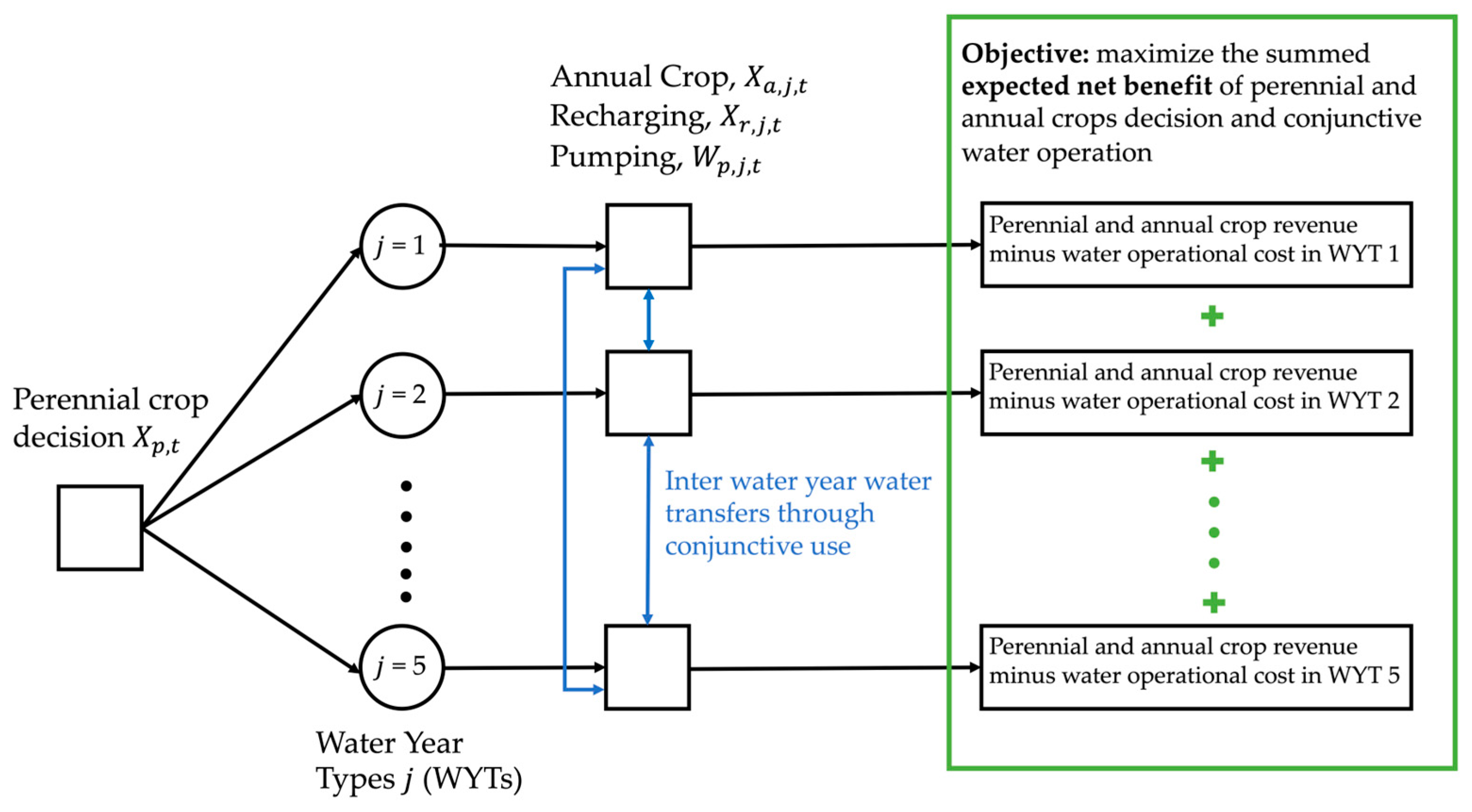
Figure 1. Problem decision tree of the inner model.
Water 16 01223 g001
Figure 2. Case aquifer illustration, where L is the total available area (Equation (2)); Ho and Bo are the initial pump head and thickness of the aquifer, respectively (Table 1 and Equation (A6) in Appendix A).
Water 16 01223 g002
Figure 3. Surface water inflow of each water year type (WYT).
Water 16 01223 g003
Figure 4. Crop water requirement and conjunctive water use decisions for different 10-year expected groundwater storage change.
Water 16 01223 g004
Figure 5. Comparison of cropping and conjunctive water operation decisions for different initial groundwater storages under no overdraft (∆GW = 0).
Water 16 01223 g005
Figure 6. Pumping in earlier decades increases with higher discount rates, delaying groundwater recovery (Initial groundwater storage is 14.8 billion m3 with a 12.3 billion m3 final goal).
Water 16 01223 g006
Figure 7. Longer-term multi-decade DP-hybrid optimization in decade 1 increases perennial cropping and decreases pumping and annual crop acreage compared to more myopic single-decade optimization. (a) If no overdraft is allowed, multi-decade decisions still have more perennial crops with more pumping and artificial recharge; (b) with net pumping allowed, long-term multi-decade decisions pump less but grow more perennial crops.
Water 16 01223 g007
Figure 8. Comparison of cropping and pumping decisions with different climates under no overdraft (∆GW = 0).
Water 16 01223 g008
Figure 9. Change in groundwater storage (dotted lines) and perennial crop acreage (Xp, solid lines) in each decade for different climates.
Water 16 01223 g009
Table 1. Input parameters of the case study site.
SymbolParameterValue (Unit)
TLength of planning horizon10 (yr)
LTotal available area202,343 ha (500,000 acre)
HoInitial pump head60.96 m (200 ft)
BoInitial thickness of the aquifer60.96 m (200 ft)
syAquifer specific yield0.1
rConstant discount rate for inner model3.5%
inipPerennial crop initial establishment cost$29,653/ha ($12,000/acre)
clandUnit price of land for recharging$741/ha ($300/acre)
cclass1Unit price of class 1 (firm contract) water$0.034/m3 ($42/AF)
cclass2Unit price of class 2 (surplus) water$0.024/m3 ($30/AF)
class1Amount of firm contract water617 million m3/yr (500 TAF/yr)
ceUnit price of energy$0.189/kWh
ηpPumping efficiency0.7
capCapacity of land for recharging4.572 m/yr (15 ft/yr)
1 − φIrrigation efficiency0.85
Table 2. Available surface water in each water year type (WYT).
WYT jPercentileswj (Million m3/yr)pj
1 (Dry)10th3060.2
230th4780.2
3Median6490.2
470th8830.2
5 (Wet)90th13760.2
Table 3. Economic values of water ($/m3) in different WYTs in a decade for different groundwater storage restoration goals (negative ∆GW draws down the aquifer) from Lagrange multipliers on conservation of mass constraints.
GW
(Billion m3)
Economic Values of Water ($/m3)
DrySurface WaterWetGroundwater
WYT 1WYT 2WYT 3WYT 4WYT 5
−1.230.140.140.140.140.0780.031
00.170.170.170.150.0790.049
1.230.230.230.180.150.130.079
2.470.280.280.1820.1820.1820.105
Table 4. Comparison of annual crop acreage (Xa (ha/yr)) and conjunctive water use decisions (land for artificial recharge Xr (ha/yr), and pumped groundwater Wp (million m3/yr)) with different initial groundwater storage under no overdraft (∆GW = 0).
Xa (ha/yr)Xr (ha/yr)Wp (Million m3/yr)
GWt − 1 (Billion m3)12.318.512.318.512.318.5
WYT j1 (Dry)753711,14000389442
2753711,14000217271
3753711,140004699
420,27620,2760000
5 (Wet)53,69242,8830348800
Table 5. WYT probabilities in each climate.
WYT jClimates
Even DrierDrierBase
1 (Dry)0.30.250.2
20.30.250.2
30.20.20.2
40.10.20.2
5 (Wet)0.10.10.2
Expected incoming surface water (million m3/yr)591 (−20%)640 (−13%)739
Table 6. Comparison of cropping and conjunctive water operation decisions with different climates without groundwater storage change (no artificial recharge occurs for the base climate).
ClimatesEven DrierDrierBase
Xp (ha/Decade)44,15845,12347,058
Second Stage
Decisions
XaXrWpXaXrWpXaWp
(ha/yr)(ha/yr)(m3/yr)(ha/yr)(ha/yr)(m3/yr)(ha/yr)(m3/yr)
WYT j1 (Dry)18990269 × 10641420314 × 1067537389 × 106
21899098 × 10641420143 × 1067537217 × 106
3688200607100753746 × 106
422,7150021,9030020,2760
5 (Wet)52,0641312054,307327053,6920
Table 7. Economic values of water ($/m3) in different WYTs for different climates under no overdraft (∆GW = 0). Values in bold and italics indicate that pumping and artificial recharge are needed in the WYT, respectively.
ClimatesEconomic Values of Water ($/m3)
Dry Surface WaterWet Groundwater
WYT 1WYT 2WYT 3WYT 4WYT 5
Base0.170.170.170.1470.0790.049
Drier0.230.230.1770.1450.0400.053
Even drier0.280.280.1840.0720.0420.056
Table 8. Average surface water economic value change ($/m3) in 10 decades between different climates for an ending groundwater target of 12.3 billion m3 (10 MAF).
Initial Groundwater Storage GWo (Billion m3)Climate Change
Even Drier to DrierDrier to Base
9.870.360.28
11.10.340.24
12.30.300.22
13.60.280.21
14.80.270.20
Table 9. Groundwater economic value change ($/m3) in 10 decades between different climates for an ending groundwater target of 12.3 billion m3 (10 MAF).
Groundwater Storage Change (Billion m3)Climates
Even DrierDrierBase
9.87 to 11.10.0950.0870.057
11.1 to 12.30.0750.0600.046
12.3 to 13.60.0620.0510.044
13.6 to 14.80.0570.0510.043
Disclaimer/Publisher’s Note: The statements, opinions and data contained in all publications are solely those of the individual author(s) and contributor(s) and not of MDPI and/or the editor(s). MDPI and/or the editor(s) disclaim responsibility for any injury to people or property resulting from any ideas, methods, instructions or products referred to in the content.