1. Introduction
History indicates that many civilizations appeared and developed along the rivers, the prominent bones of anthropic activity, sustaining food production, transportation, and providing water for drinking and industry [
1,
2]. On the other hand, floods have often had catastrophic effects on population settlements. Therefore, learning from the past is essential to observe and understand the evolution of the water cycle and river flow dynamic. Setting an early-warning system for taking timely and informed measures to avoid (if possible) or reduce the floods of drought effects on human activities is necessary [
3,
4,
5,
6,
7,
8]. Research of the rivers’ flow was performed in different directions, as follows:
For example, statistical analysis [
34] can emphasize the series characteristics and the existence of outliers and breakpoints, determine its distribution, and test different hypotheses. It does not effectively provide a river discharge model, which is essential for a reliable forecast. To complement the findings provided by statistical analysis [
7,
8], the HEC-RAS software was used to model the susceptibility to floods in different basins. HEC-HMS was employed to simulate losses, snowmelt, sub-basin routing, and river flow routing [
35].
Rainfall-runoff modeling is a critical aspect of water management, with far-reaching implications for various hydrological processes, particularly those associated with extreme events like flooding. To account for the intricacies of the models, a range of storage parameters are fine-tuned using an extensive dataset of meteorological and hydrological information [
37]. The better the model, the better the river discharge forecast.
Various methods can predict future time series behavior, from classical decomposition models—which emphasize trend, seasonality, and random variation to Box–Jenkins methods [
8,
10,
38,
39,
40], exponential smoothing [
9], and different types of AI [
12,
20,
21,
22,
23,
24,
25] and hybrid models [
28,
29,
30,
31,
32,
33].
Traditional approaches for modeling and forecasting the river water discharge struggle with large datasets and have limitations in capturing regime changes and non-linearity. Moreover, they are based on restrictive assumptions, like normality or stationarity. By contrast, AI techniques do not impose restrictions on the data; they learn the input series quickly, are less sensitive to the outliers’ presence, and can capture abrupt changes in the datasets. These characteristics recommend them as valuable tools to forecast the series’ behavior. Comparisons of these two approaches [
12,
39,
41] indicated superior reliability of AI models. Among them, extreme learning machines (ELM) [
42,
43] proved fast learning features [
44]. LSTM [
45] can capture the series’ long-range dependence, incorporating historical information by automatically learning the data and extracting its future [
46]. Backpropagation neural networks (BPNN) proved to be a valuable tool in water-level prediction and were proposed for modeling the river’s water discharge [
47,
48]. Still, there are not enough studies to prove its performance in this research field.
Hydrotechnical structures, such as dams and reservoirs, are crucial for addressing human needs. However, they can significantly alter natural rivers’ flow [
49,
50,
51], sometimes leading to substantial environmental damage and declining biodiversity. Reducing the flood effects on the anthropic settlements was a practical problem that needed to be solved, and it was a study direction for different researchers. Some analyzed the dam’s environmental effect, emphasizing the river flow alteration [
8,
12,
52,
53,
54,
55,
56]. A deep study of the impact of such structures may contribute to understanding this phenomenon and taking measures to reduce the effects of natural calamities.
The Siriu Dam was built on the upper reach of the Buzău River, one of the most important rivers in Romania, to regulate water flow; reduce the effect of floods on the people living in its catchment; and provide water for drinking, irrigation, and industry. Its importance has not yet been emphasized enough. In Romania, only a few researchers investigated the change in the river flow regimen after the dam inauguration [
53,
54,
55]. Moreover, the research of rivers’ dynamics by AI methods is insignificant, the most utilized tools being statistical methods and hydraulic modeling [
5,
6,
7,
53,
54,
55].
The present study is in line with the international literature. Its novelty consists of:
Providing alternative models for the Buzău River discharge before and after building the dam using AI algorithms;
Pointing out the modification of the river flow alteration after the dam apparition;
Exploring the BPNN, LSTM, and ELM capacity for modeling the water river discharge on series with high variability and outliers. These techniques were selected due to their advantages in modeling time series from various research fields [
42,
43,
44,
45,
46,
47,
48]. Moreover, we aimed to prove their performances in hydrological modeling (where they were less used compared to other approaches).
Comparing the single and hybrid AI techniques in hydrological modeling.
2. Study Area and Data Series
Buzău River is one of Romania’s most prominent water bodies. The Buzău River’s catchment (5264 km
2 and 1043 m average elevation) (
Figure 1 (left)) belongs to the Curvature Carpathians, where the climate is temperate—continental. More than four-fifths of the yearly water volume flows upstream of Nehoiu. Catastrophic floods were recorded in the Buzău catchment from 1948, with a maximum discharge of 2100 m
3/s in 1975 (one hundred times higher than the average monthly discharge). The Siriu Dam was inaugurated on 1 January 1984. It altered the river’s water discharge and positively impacted the community, reducing the number and intensity of flooding events [
55,
56].
The monthly discharge series from January 1955 to December 2010 (
Figure 1 (top right)), denoted in the following by S, are official data from the National Institute of Hydrology and Water Management (INGHA) and contain no missing value.
Figure 1 (bottom right) provides the basic statistics of series S and the subseries from January 1995 to December 1983, before building the dam, and from January 1984 to December 2010, after building the dam. Min, Max, and Mean (m
3/s) are the minimum, maximum, and mean values. CV, Skew, and Kurt (dimensionless) represent the coefficient of variance, skewness, and kurtosis.
The Mann–Kendall and seasonal Mann–Kendall trend tests did not reject the randomness hypothesis for the monthly series S. Still, they rejected it for the sub-series before December 1983 and after January 1984. The linear trend slopes computed by Sen’s method are 0.0139 for the subseries before December 1983 and 0.0311 for the subseries January 1984–December 2010. So, there is an increasing trend in the river discharge for both subseries but not for the entire series. This result indicates different long-term tendencies of the monthly subseries. The KPSS test did not reject the stationarity hypothesis for all series.
More details on the statistical analyses performed on the monthly Buzău River water discharge may be found in [
53,
54,
55].
3. Methods
Machine Learning (to which the three algorithms mentioned above belong) is a technique where a computer algorithm can automatically learn from data and make predictions or decisions based on that learning. The typical procedure involves dividing a study series into two parts: the Training set and the Test set. The Training set feeds the algorithm with a dataset, allowing it to learn the relationship between the input features and the target variable. During this stage, the algorithm updates its parameters until it can accurately predict the target variable for new, unseen data. Once the training is complete, the model’s performance is evaluated by testing its accuracy on previously unseen data. The Test set objectively measures how well the model performs on new data. The results help to determine if the model is overfitting (performs well on the Training dataset and poorly on the Test set) [
57,
58].
For our study, we standardized the variables. This study employed the BPNN, LSTM, and ELM algorithms. The Test and Train sets for the models are presented in
Table 1.
Random seeds are essential in computational models involving random search methods like Machine Learning. Their selection can impact the weight initializing and choosing the data sets at different stages of the algorithm. Therefore, setting the same seed is a solution to ensure the reproducibility of the results. To correctly assess the models’ performances, they were run with various seeds, which were kept constant in a cycle for all three algorithms.
After obtaining the outputs, the quality of the models was evaluated using the mean absolute error (MAE), mean squared error (MSE), and coefficient of determination (R2) for both Training and Test sets. The lower (higher) the MAE and MSE, or the closer to 100% (0%) the R2, the better (worse) the model is.
To perform the study, we employed Matlab R2023a under Windows 11. The workstation details are as follows: AMD Ryzen 9 5900X 12-Core Processor CPU (3.70 GHz, 12 cores, 24 threads), 64 GB of RAM, NVIDIA GeForce RTX 3090 GPU.
In the following, we present the algorithms involved in computation and the setting used in this study.
3.1. BPNN
A particular type of feed-forward neural network is represented by BPNN [
58]. It is an ANN with multiple layers that utilizes the backpropagation algorithm [
59] in the learning process. The network is formed by the input, hidden, and output layers. All neurons from the input layer are connected to those in the hidden layer. Weights (w) are assigned to each neuron. The ReLU or sigmoid is used as an activation function. Each input element passes to the next layer, where the new value is computed as a weighted average of the input values in each neuron. Then, it passes to the output layer after applying the activation function [
60].
The deviation of the computed values from the recorded ones is measured by the loss function, f, which is MSE. The backpropagation algorithm employed by BPNN updates the weights and minimizes the value of f. The error appearing in the hidden layer is calculated utilizing the chain rule based on the error previously computed for the output layer. The iterations are repeated until the loss function’s convergence or the maximum number of iterations previously established is reached. The forecast of the data series is performed only after the training step.
The parameters used to run the BPNN are given in
Table 2. In the BPNN model, we utilized for training the Momentum Gradient Descent algorithm, a variant of the standard gradient descent algorithm that accelerates convergence by adding a fraction of the previous update vector to the current update, thereby reducing oscillations and achieving faster convergence.
The learning rate determines the step size during weight updates in optimization. A suitable learning rate is crucial for achieving convergence without overshooting the optimal solution. We used the sigmoid activation function to introduce non-linearity into the network, enabling it to learn and approximate complex relationships within the data.
3.2. LSTM
LSTM [
45] is a type of recurrent neural network (RNN) that uses gates to control the flow of information into and out of the network. It also contains a memory cell that keeps information for an extended period. The memory cell works under the control of the Forget, Input, and Output Gates. The Forget Gate selects the information to be discarded from the memory cell, whereas the Input Gate determines what must be added. The Output Gate controls the memory cell’s output. This structure allows LSTM to learn long-term dependencies.
The architecture of an LSTM is chain-type with units (
Figure 2).
The equation that governs the Forget Gate’s functioning at a moment
j is [
45,
61,
62,
63,
64]:
where
is the Forget Gate unit at
j,
is the matrix of the weights of Forget Gate,
is the input at
j,
is the hidden state at
j − 1,
is the Forget Gate bias at
j, and
is the sigmoid activation function (whose output is 0 or 1, meaning that the information is forgotten or retained).
The Input Gate working at a moment
j is performed by:
where
is the Input Gate’s unit at
j,
is the matrix of the weights of the Input Gate, and
is the bias of the Input Gate at
j.
In the Input Gate, information passes through a sigmoid function that decides the values to be updated. After that, a hyperbolic tangent function (tanh) builds the new candidates’ vector:
where
is the candidates’ vector,
is the matrix of the weights of the candidates’ vector, and
is the candidates’ vector’s bias at
j.
The equation employed in the update unit to update the information is the following:
where ∗ is the element-wise multiplication.
The Output Gate functioning at a moment
j is described by:
where
is the Output Gate unit at
j,
is the matrix of the Input Gate weights, and
is the Output Gate bias at
j.
The actual hidden state is calculated by:
The parameters used to run LSTM are presented in
Table 3.
To train the LSTM network, we utilized the Adam optimizer. Adam is an adaptive learning rate optimization algorithm that combines ideas from momentum and RMSProp methods. It dynamically adjusts the learning rate based on past gradients, leading to faster convergence and improved performance. The batch size used during training, which determines the number of samples processed before updating the model’s parameters, was 64. This choice was made to strike a balance between computational efficiency and model convergence. We also conducted tests with 32 and 16, but the best results were obtained with 64.
The dropout regularization technique was applied to prevent overfitting by randomly deactivating a fraction of neurons during training.
3.3. ELM
ELM [
42,
43,
65] is a feed-forward neural network for supervised learning tasks. Its core principles involve the initialization of a neural network and weight learning. ELM has three layers: input, hidden, and output.
The input of the input layer is a vector X of an established dimension (d). The matrix of the weights, W, is randomly initialized in the hidden layer. The hidden layer’s output is obtained by passing the product (b is the bias) through an activation function.
ELM employs the least squares method to learn the weights (
O) in the output layer. The
O matrix is computed by multiplying the Moore–Penrose pseudo-inverse of the hidden layer output matrix with the class label matrix [
66].
The forecast of a vector
X’ is performed by the formula:
where
is the weights matrix from the hidden layer to the output layer.
The results from [
41,
42] indicate that ELM learns quickly and can act as a universal approximator. ELM is particularly useful when dealing with large datasets because it can train models faster than traditional algorithms. It also has good generalization capacity, so it can make accurate predictions on new, unseen data [
66,
67].
The parameters utilized to run ELM are shown in
Table 4.
No specific optimization algorithm was used as the traditional training process of ELM involves randomly initializing the input weights and biases, followed by computing the output weights analytically. Therefore, no iterative optimization process is involved in training ELM.
We used the sigmoid activation function in ELM to introduce non-linearity.
4. Results and Discussion
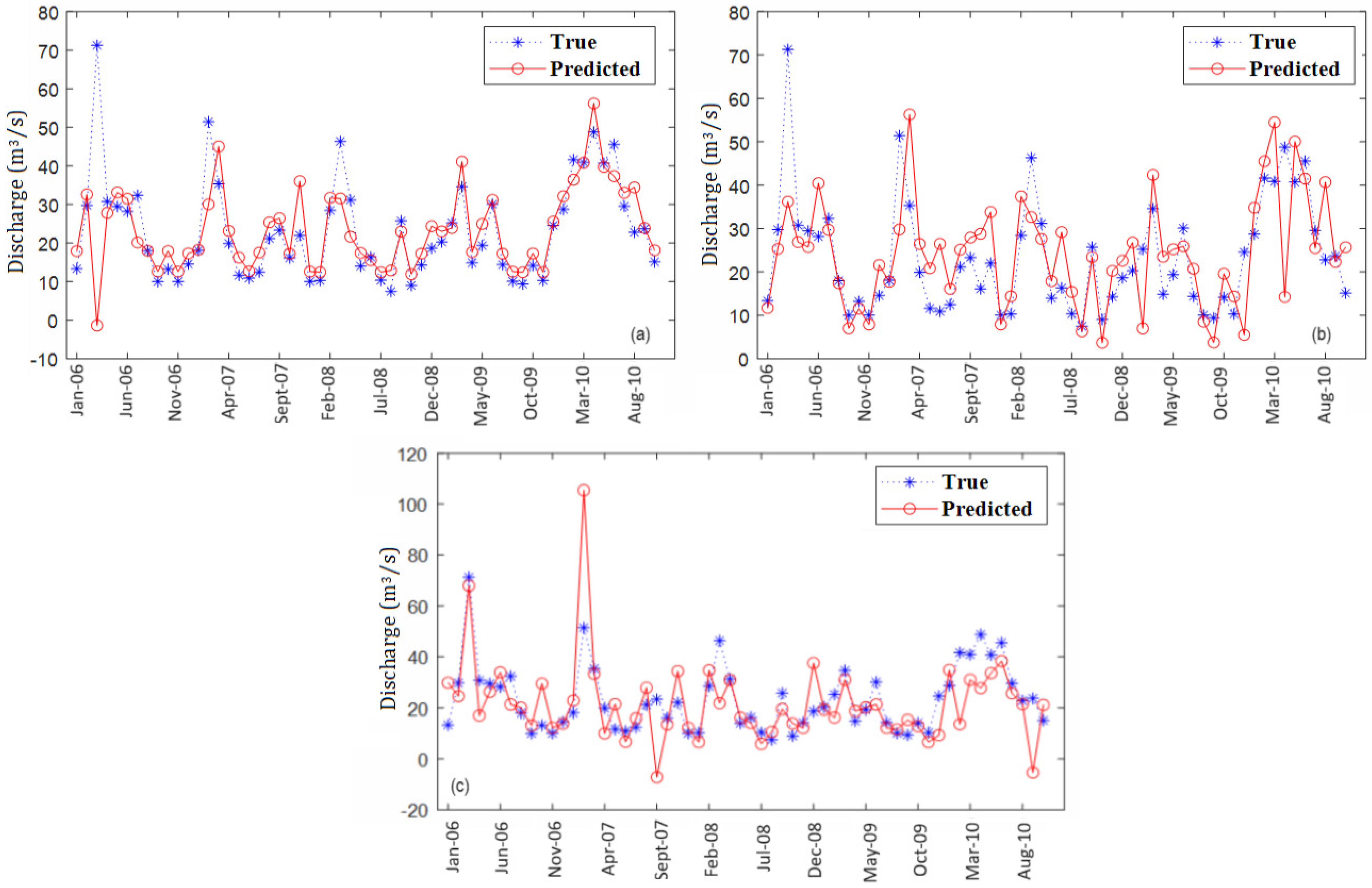
Figure 3,
Figure 4 and
Figure 5 display the recorded and predicted values of the Test set after running BPNN, LSTM, and ELM, respectively, according to the segmentation from
Table 1.
Figure 3a shows a high bias between the recorded and computed values in March 2006, February 2006, March 2008, and June 2010 and the discordant behavior of the actual and estimated trend in the neighboring periods. By comparison, in
Figure 3b, most values are overestimated, and the estimation errors (difference between the recorded and computed values) are bigger. In
Figure 3c, the highest differences between the two series appear in February and September 2007 (56 and 34.5 m
3/s, respectively) and February and September 2010 (34 and 29 m
3/s, respectively). The visual examination shows that the best fit is provided in
Figure 3a. Still, the error from March 2006 (about 72 m
3/s) significantly increases the MAE and MSE (that uses the squared errors in computation).
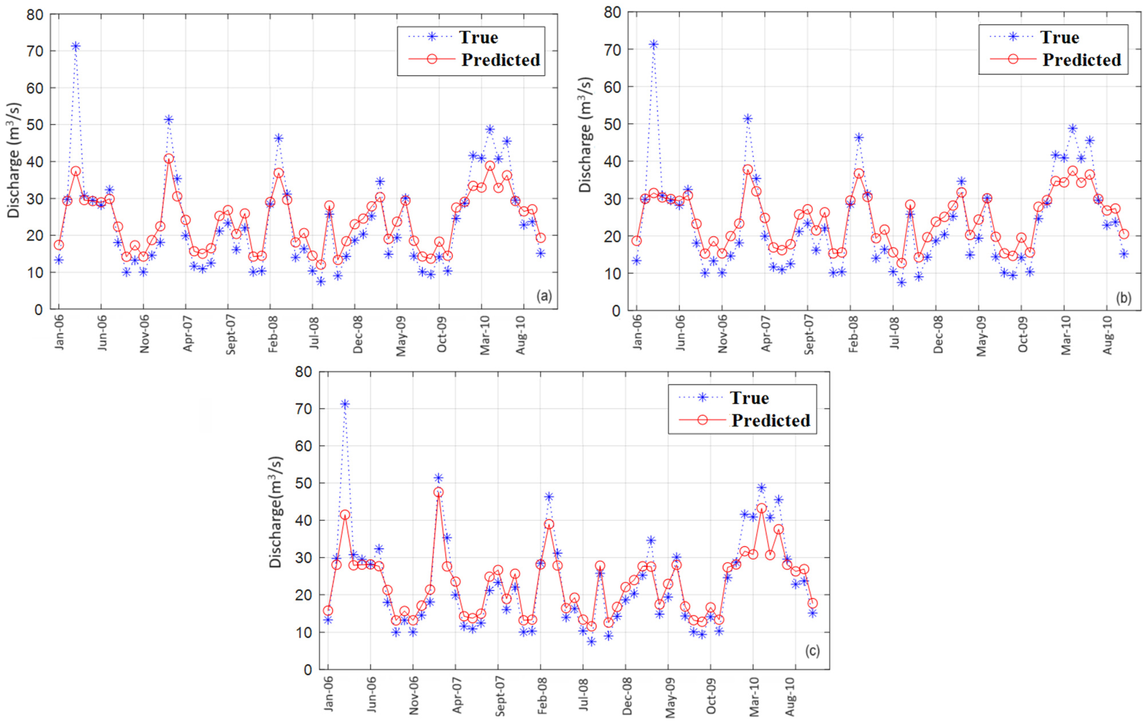
Compared to the BPNN, the LTSM models (
Figure 4) capture the recorded series pattern better. More precisely, there is no deviation of the forecast trend from the recorded one.
Given that the maximum values of the raw series are underestimated, and some of the minima are overestimated (in
Figure 4b), the values of MAE and MSE will not be very small. The forecast series from
Figure 4b is the smoothest, so it is expected to have the highest errors compared to
Figure 4a,c.
The ELM models (
Figure 5) exhibit the highest capacity of capturing the maxima with respect to the competitors. At the same time, the overestimation of the minima is smaller than in the case of BPNN and LSTM, especially for S2. In all cases, the patterns of the original series are entirely captured.
After a visual examination, the output of the ELM algorithm is the best among the three approaches. To confirm this assertion, the goodness-of-fit indicators were computed and are presented in
Table 5.
The MAE varied between 4.01 (ELM on the S2 Test set) and 11.00 (BPNN on the S1 Training set). All MAEs corresponding to the Training set are higher than those for the Test one, except for S2 on BPNN, indicating that in most cases, the algorithms perform better on the Test sets. In terms of MAE, the best results were given by utilizing ELM: MAE = 5.02 (on the training set) and MAE = 4.01 (on the Test set) on S2. The highest MAEs were 11.00 and 7.94—BPNN on S1 on the Training and Test set, respectively. So, ELM exhibits the best performance. LSTM occupies the second place.
The MSE range is much higher given the existence of the maxima that need to be fitted better, as explained below. On the Training set, MSE varied between 60.07 (S2—LSTM) and 326.62 (S1—BPNN).
On the Test set, MSE belonged to the interval 32.21 (S2—ELM)—158.55 (S2—BPNN). So, in terms of MSE, ELM performed the best on the Test set for S, S1, and S2, and the Training set on S1, whereas on the Training sets for S and S2, the best was LSTM.
R² obtained low values in the BPNN model, indicating a reduced concordance between the recorded and forecast series. The values of R2 were significantly higher in the ELM approach, belonging to the intervals [76.14%, 83.05%] on the Training set and [81.84%, 90.71%] on the Test set. In terms of R2, the best performance was achieved by the LSTM algorithm. In this case, R2 is in the interval [98.99%, 99.97%], pointing out the almost perfect correlation between the actual and predicted values on both Training and Test sets.
Comparing the algorithm capabilities on S, S1, and S2, the best-fitted series is S2. A possible explanation is that S2 is trained, and the forecast is made with values from the same period (after January 1984—the dam inauguration) compared to the model for S, which is trained with values from both periods (before and after building the dam). The fit quality of S1 can be the consequence of the high variability of the river discharge before 1984, attenuated after 1984.
The outputs of algorithms run on S and S1 indicate a better fit in the first case, results expected since S1 was trained on unaltered discharge (before January 1984), but the prediction was made for altered river flow (after January 1984). These findings are concordant with those from [
62].
The results reflect the LSTM’s ability to capture series nonstationarity and non-linearity, remember information from a long past, and discard irrelevant data. On the other hand, they also indicate the ELM’s good generalization capacity [
41,
42].
Another aspect that was considered is the computation cost (
Table 6). Known as a fast learning feed-forward algorithm [
41], the ELM achieved the lowest run time. The longest time corresponds to the LSTM on the S series (the longest one), followed by LSTM on S2 and S1 (that have almost the same length). Details on the time complexity of each algorithm can be found in [
45,
68,
69,
70].
Comparison of the actual approaches with the existing results on the same data series [
62] indicates the following:
ELM and PSO-ELM perform similarly with respect to all goodness-of-fit indicators. The run time is significantly lower for ELM than that of PSO-ELM (358.07 s for S, 56.43 s for S1, and 50.13 (or S2).
LSTM was more accurate than CNN-LSTM in terms of R2 and MSE for S and S2. The run time for LSTM was 2.35 (1.63) times lower than that of CNN-LSTM for S (S2).
All algorithms perform better than multi-layer perceptron (MLP) and the Box–Jenkins (ARIMA) models for S, S1, and S2.
These results confirm the suitability of LSTM for modeling hydrological series [
71,
72] and point out the ELM [
73,
74] as a possible competitor in solving such problems.
5. Conclusions
The research presented here examined the performances of three AI models for forecasting the Buzău River water discharge for 572 months and subperiods before and after building the Siriu dam and pointed out the river flow alteration after 1984 without using statistical tools. It also compared the goodness of fit of BPNN, LSTM, and ELM with the same series’ PSO-ELM, CNN-LSTM, MLP, and ARIMA models.
This research makes a unique contribution to the field by testing the performances of the first three mentioned algorithms on the river flow series. This novel approach aims to enhance their abilities to learn patterns and forecast datasets with high variability, thereby introducing a new dimension to the field of water resource management.
Various performances of different algorithms were expected, given their architectures and functioning. ELM performed best in terms of MAE (between 4.01 (S2—Test) and 6.79 (S1 Training)) and MSE (between 32.21 (S2—Test) and 98.79 (S1—Training)). With respect to R2, ELM placed second, with values between 79.71% (S—Training) and 89.71% (S2—Test), after LSTM, with R2 in the interval 98.99% (S1—Training) and 99.97% (S2—Test). ELM was also the fastest, with a runtime under 0.75 s in all cases, indicating that it quickly learns of the series patterns and accurately applies what it knows. LSTM confirmed its capacity to preserve the long-term essential information and its good reproduction capacity of the non-linearities in the data series. By comparison with the ELM, it was at least six times slower.
Given that ELM is the best based on MAE and MSE, has a low computational cost, and has a high R2, it is recommended to achieve the study objective.
The second novelty is comparing single and hybrid models on the same data series. Based on R2 and MSE, LSTM is better than the hybrid competitors and has a significantly lower computational cost. So, it is recommended for modeling the study series. The worst performances among all techniques were those of MLP and ARIMA. These findings reconfirm the capacity of AI methods in forecasting modeling hydrological series.
One of the things learned from these models is that not all AI algorithms have the ability to predict with very high accuracy any changes in river flow due to external effluences such as a dam. Moreover, AI models should be incorporated into physical models to be of value beyond the traditional models when changes occur in the watershed.
The best results were obtained on S2 (the shortest series), for which both Training and Test sets belong to the same period (after January 1984). The worst models’ performances were achieved on the S1, for which the Training was performed on a dataset before December 1983 and the Test on a dataset after January 1984. This proves that the pattern learned in the first set is not the same as that of the second one, so the alteration of the river flow was significant after building the dam.
The next stage of the work is to apply the same techniques to daily data series. Given the computational complexity, we expect some algorithms to have high run times and require more powerful computational tools. Moreover, data preprocessing will be necessary, given the episodes of high flows that were not captured by the monthly series.


