Abstract
Computing the temporal variation in clearwater scour depth around abutments is important for bridge foundation design. To reach the equilibrium scour depth at bridge abutments takes a very long time. However, the corresponding times under prototype conditions can yield values significantly greater than the time to reach the design flood peak. Therefore, estimating the temporal variation in scour depth is necessary. This study evaluates multiple machine learning (ML) models to identify the most accurate method for predicting scour depth (Ds) over time using experimental data. The dataset of 3275 records, including flow depth (Y), abutment length (L), channel width (B), velocity (V), time (t), sediment size (d50), and Ds, was used to train and test Linear Regression (LR), Random Forest Regressor (RFR), Support Vector Regression (SVR), Gradient Boosting (GBR), XGBoost, LightGBM, and KNN models. Results demonstrated the superior performance of AI-based models over conventional regression. The RFR model achieved the highest accuracy (R2 = 0.9956, Accuracy = 99.73%), followed by KNN and GBR. In contrast, the conventional LR model performed poorly (R2 = 0.4547, Accuracy = 57.39%). This study confirms the significant potential of ML, particularly ensemble methods, to provide highly reliable scour predictions, offering a robust tool for enhancing bridge design and safety.
1. Introduction
Scour around bridge abutments represents a critical structural safety concern within the domain of hydraulic engineering. The removal of bed material around the abutments can compromise the integrity of the bridge foundation, potentially leading to structural instability or collapse over time [1]. Reaching the equilibrium scour depth around bridge abutments takes a very long time; it may take many days, even months. Since floods typically last for a much shorter duration than the time required to reach the equilibrium state of scour holes, studying the time variation in scour depth is crucial. In this study, the time development of scour holes around the abutments was investigated by machine learning methods. Beyond the equilibrium scour depth, each scour depth at a given time was estimated by machine learning techniques. Estimated values were compared with the data gathered from the literature that was obtained experimentally.
Traditionally, the prediction of scour depth has relied on empirical formulas and physical modeling techniques. Foundational research by Melville and Coleman introduced key empirical correlations based on hydraulic parameters for estimating scour depth [2]. In addition, guidelines such as the HEC-18 manual issued by the Federal Highway Administration have been widely adopted in engineering practice. However, these conventional methods often fall short in adapting to diverse site conditions and may lack precision in their predictive capabilities [3].
With the increasing use of artificial intelligence (AI) and machine learning (ML), more advanced approaches have come into consideration for scour depth estimation. The studies performed by Lee et al. and Azamathulla et al. have demonstrated that models such as Support Vector Machines (SVMs) and Artificial Neural Networks (ANNs) are effective in capturing the complex and nonlinear relationships between hydraulic factors and scour depth [4,5]. Moreover, ensemble learning methods like Random Forest and XGBoost have demonstrated enhanced performance in terms of both accuracy and generalization [6].
Hamidifar et al. demonstrated that hybrid models, which integrate empirical equations with machine learning algorithms, yield more reliable scour depth predictions [7]. Similarly, Khan et al. found that AI-based methods outperformed traditional approaches in terms of prediction accuracy. Collectively, these findings underscore the increasing relevance and effectiveness of AI-powered models in modern hydraulic engineering practices [8].
Mohammadpour et al. utilized both Adaptive Neuro-Fuzzy Inference System (ANFIS) and Artificial Neural Network (ANN) techniques to estimate the temporal development of scour depth around structural foundations [9]. Similarly, Choi et al. recommended the use of the ANFIS approach for predicting scour depth around bridge piers [10]. In another study, Hoang et al. developed a machine learning model based on Support Vector Regression (SVR) to forecast erosion on complex scaffolds subjected to steady clear-water conditions [11]. Abdollahpour et al. applied Gene Expression Programming (GEP) and Support Vector Machine (SVM) algorithms to investigate the geometric characteristics of erosion downstream of W-shaped dams in meandering channels [12]. Furthermore, Sharafati et al. introduced a hybrid modeling framework that combines Invasive Weed Optimization (IWO), Cultural Algorithm, Biogeography-Based Optimization (BBO), and Teaching-Learning-Based Optimization (TLBO) with ANFIS to estimate the maximum scour depth [13]. Ali and Günal implemented ANN-based prediction models on various datasets to improve erosion forecasting performance [14]. Lastly, Rathod and Manekar applied a Gene Expression Programming (GEP) technique rooted in artificial intelligence to design a comprehensive and adaptable erosion model suitable for both laboratory experiments and real-world field conditions [15]. Accurate prediction of scour depth (Ds) is essential to ensure the structural safety and longevity of bridges under clear-water flow conditions. Although various approaches, such as empirical formulas and physical modeling techniques, have been developed for estimating scour depth in such environments, these methods often suffer from limited generalizability. Their applicability is typically constrained by site-specific conditions and the relatively small datasets on which they are based.
In recent years, significant progress in artificial intelligence (AI) and machine learning has enabled the accurate modeling of complex hydraulic phenomena. These data-driven approaches are particularly effective at identifying nonlinear relationships among variables by leveraging large datasets, thereby offering more reliable and robust predictions. Traditionally, scour depth estimation has been achieved using empirical formulas or hydraulic laboratory experiments. However, these methods often fail to fully capture complex hydrodynamic processes and are difficult to model scour dynamics that vary over different timescales. In recent years, machine learning techniques have been increasingly used in hydraulic engineering problems due to their ability to provide highly accurate predictions.
The main purpose of this study is to determine the most suitable machine learning model for predicting the time-dependent scour depth (Ds) around bridge abutments. Unlike previous studies, comprehensive comparisons of seven machine learning algorithms Linear Regression (LR), Random Forest Regressor (RFR), Support Vector Regression (SVR), Gradient Boosting Regression (GBR), XGBoost, LightGBM (LGBM), and K-Nearest Neighbors (KNN), were conducted using a dataset compiled from the literature. Key hydraulic parameters, including flow depth (Y), abutment length (L), channel width (B), flow velocity (V), time (t), and median grain size (d50), were used as inputs to predict Ds. The models were evaluated using standard metrics such as Mean Squared Error (MSE), Root Mean Squared Error (RMSE), and the Coefficient of Determination (R2), and their predictions were compared against experimental data.
The study’s findings will provide data-driven guidance to decision-makers in bridge design and risk management and establish a new reference for future research.
2. Materials and Methods
2.1. Local Scour
The primary mechanism responsible for local scour at bridge abutments is the development of vortices near the abutment base, as illustrated in Figure 1 [16]. These vortices lead to degradation by transporting sediment from the tip of the abutment. When the rate of sediment degradation exceeds the rate of aggradation of bed material, a scour hole occurs. Additionally, wake vortices, down flows, and horse-shoe vortex occurring downstream of the abutment contribute to sediment transport. However, the influence of wake vortices diminishes rapidly as one obtains away from the abutment base. Typically, the depth of local scour significantly exceeds that of general or contraction scour, often by an order of magnitude [3].
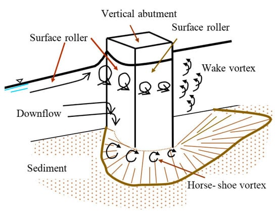
Figure 1.
Abutment scour phenomenon [17].
All experimental data used in this study belonged to the abutment configured as a vertical abutment. Representative measurement sections for abutment scour depth (Ds) and the time variation in scour are illustrated in Figure 2.
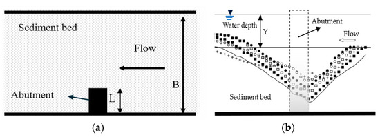
Figure 2.
Placement of abutment in the channel and time variation in scour hole in the experimental setup: (a) plan view, (b) cross-sectional view.
In order to visually demonstrate the time variation in local scour development around bridge abutments, an experimental study was carried out at the Technical Research and Quality Control Laboratory of the General Directorate of State Hydraulic Works. Time variation in local scour formation was observed under controlled conditions with the following parameters: channel width (B) = 1.5 m, abutment length (L) = 20 cm, flow discharge (Q) = 0.38 m3/s, mean sediment diameter size (d50) = 1.48 mm, and flow depth (Y) of 10 cm, shown in Figure 3.
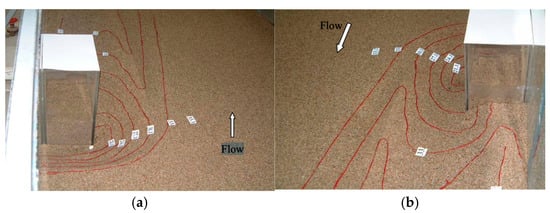
Figure 3.
Time variation in scour hole development observed in the experimental study: (a) upstream view; (b) downstream view.
2.2. Parameters Influencing Scour Around Bridge Abutments
The descriptions of key factors influencing the extent of local scour at bridge abutments are provided below [16]:
- Flow Velocity (V): An increase in flow velocity leads to a stronger scouring force. Therefore, the dataset includes a broad range of flow velocities to capture this effect accurately.
- Flow Depth (Y): Depending on the abutment geometry, an increase in flow depth may amplify scour depth by approximately 1.1 to 2.15 times [3].
- Abutment Length (L): Longer abutments tend to produce greater scour depths due to the larger flow obstruction and channel contraction.
- Bed Material Characteristics: Properties such as grain size distribution and cohesiveness of the sediment significantly influence the scour process.
- Abutment Geometry: A streamlined abutment shape can weaken the intensity of the horseshoe vortex at the abutment base, thereby reducing the depth of local scour.
2.3. Parameters Influencing Scour Around Bridge Structures
Under clear-water flow conditions, the scour depth (Ds) around a bridge abutment is governed by hydraulic variables as expressed in Equation (1):
where L = abutment length, B = abutment width, V = mean approach flow velocity, Y = flow depth, S = slope of the channel, g = gravitational acceleration, ρs = sediment density, ρ = fluid density, μ = dynamic viscosity of fluid, d50 = median particle grain size, geometric standard deviation of sediment size distribution is defined as σg = (d84/d16)0.5 (where d84 = is the grain size for which 84% of the material is finer, d16 = is the grain size for which 16% is finer), and t = scouring time.
The dimensionless form of the scour depth can be represented by Equation (2):
By neglecting the effects of bed slope, experiment duration, and fluid viscosity, the relationship can be simplified as shown in Equation (3):
where the scour depth (Ds) is expressed in a dimensionless form, normalized by the flow depth (Y).
2.4. Dataset
The dataset used in this study consisted of the experimental measurements taken from the literature [9,18,19,20,21,22,23,24,25]. These measurements included scour values recorded over time, allowing for the estimation of time-dependent scour depth (Ds) variation.
In this study, the evaluation and prediction of the results were performed using various machine learning methods, including Linear Regression (LR), Support Vector Regression (SVR), Random Forest Regressor (RFR), XGBoost, Gradient Boosting (GB), LightGBM (LGBM), and K-Nearest Neighbors (KNN). The dataset used in this study consists of 3275 data records.
Table 1 shows the characteristics and measurement limits of the dataset used in the study.

Table 1.
Main characteristics of the experimental studies and limits of the experimental dataset.
2.5. Linear Regression
Linear Regression (LR) is a statistical technique that models the linear relationship between a dependent variable and one or more independent variables. The basic assumption of the model is that the target variable can be predicted by a linear combination of independent variables. It is expressed mathematically as Equation (4) [26]:
where represents the estimated value, xi represents the independent variables, βi represents the regression coefficients, and ε represents the error term. The model is trained using the Ordinary Least Squares (OLS) method to minimize the sum of the error squares. Although the advantages of Linear Regression include interpretability and fast calculation, it should not be forgotten that the model may be inadequate in the presence of nonlinear relationships in the data. The machine learning workflow for Linear Regression is provided in Supplementary Figure S1.
2.6. Support Vector Regression
Support Vector Regression (SVR) is a machine learning technique grounded in the principles of Support Vector Machines (SVMs), offering an alternative to conventional regression models [27]. Rather than fitting a simple linear function, SVR projects data into a higher-dimensional feature space using kernel functions, enhancing prediction capability for both linear and nonlinear relationships. Unlike ordinary Linear Regression, SVR performs estimation by incorporating a margin of tolerance known as the ε-tube, allowing predictions within this boundary.
The general representation of the SVR model is given in Equation (5):
where X is denotes the vector of independent variables (Y, L, B, V, ), w is the weight vector, b is the bias term of the model, and f(X) corresponds to the predicted value of the dependent variable (Ds).
To evaluate prediction errors, SVR applies the ε-insensitive loss function, which disregards deviations that fall within the defined ε margin and focuses solely on minimizing errors beyond this threshold. The loss function is illustrated in Equation (6) [28].
The parameter ε serves as a hyperparameter that defines the model’s tolerance threshold, essentially controlling its sensitivity. To effectively capture nonlinear relationships, SVR employs kernel functions through the so-called kernel trick. Commonly utilized kernel types include the following [28]:
- Linear Kernel: ⟨Xi, Xj⟩.
- Polynomial Kernel: (γ⟨Xi, Xj⟩ + r)d.
- Radial Basis Function (RBF) Kernel: exp(−γ‖Xi−Xj‖2).
In this study, the RBF kernel is adopted for training the SVR model. Model performance will be assessed using Mean Squared Error (MSE), Root Mean Squared Error (RMSE), and Coefficient of Determination (R2) metrics. SVR is particularly effective even with limited sample sizes, as it is resistant to noise and less prone to overfitting. Its capacity to model complex, nonlinear relationships is enhanced by its use of kernel functions. However, for larger datasets, training time may increase significantly.
To optimize performance and avoid overfitting, the grid search technique was applied to tune hyperparameters. In this context, the SVR model was configured with an RBF kernel, a regularization parameter C set to 10, and an ε value of 0.1. The predictive ability of the SVR model in estimating equilibrium scour depth will be evaluated by comparing it with other machine learning algorithms. The machine learning workflow for Support Vector Regression is provided in Supplementary Figure S2.
2.7. Random Forest Regressor
The Random Forest Regressor (RFR) is an ensemble-based machine learning algorithm that relies on a collection of decision trees. Rather than depending on the output of a single decision tree, RFR enhances prediction performance and generalizability by aggregating the outputs of multiple trees. This ensemble strategy helps mitigate overfitting and improves the overall accuracy of the model [29].
Random Forest operates using the Bootstrap Aggregation (bagging) technique, where multiple decision trees are trained on different subsets of the data generated through random sampling with replacement. The core phases of the algorithm include data resampling (bootstrapping), training of individual trees, and combining their outputs to generate final predictions [30].
By averaging the predictions from several decision trees, the Random Forest algorithm reduces the high variance often associated with single decision trees, resulting in a more stable and reliable predictive model.
The final output of the Random Forest is obtained by computing the average prediction from M individual decision trees, as shown in Equation (7):
where ŷ represents the final predicted value, M denotes the total number of decision trees, and fm(X) is the output of the mth decision tree.
Each tree in the ensemble selects the optimal feature for splitting by minimizing the Mean Squared Error (MSE) at each node. The objective is to identify the feature that results in the lowest error at each decision point.
Thanks to its bagging-based structure, the Random Forest algorithm is robust against overfitting and demonstrates strong performance in capturing nonlinear patterns. Additionally, it can assess feature importance, indicating the relative influence of each input variable on the model’s predictions. However, certain limitations exist: training time can be considerable, particularly when a large number of trees are used with extensive datasets; the model’s interpretability diminishes as it becomes harder to trace decision pathways across many trees; and computational cost may rise with the increasing number of trees [30].
In this study, the Random Forest Regressor will be employed to predict the scour depth (Ds) around bridge side abutments. Its performance will be compared with other regression algorithms using MSE, RMSE, and R2 as evaluation metrics. The machine learning workflow for Random Forest Regressor is provided in Supplementary Figure S3.
2.8. XGBoost
XGBoost (Extreme Gradient Boosting) is a highly effective ensemble learning algorithm that utilizes decision trees as its base learners. Built on the concept of boosting, it constructs a strong predictive model by combining the outputs of multiple weak learners. Known for its speed, scalability, and optimized performance, XGBoost has become a popular choice for both regression and classification tasks [31].
This method employs a Gradient Boosting framework, where decision trees are trained in sequence to minimize the overall prediction error. Initially, the model makes a rough prediction-typically by calculating the mean of the target variable (Dse). For each observation, the residual (i.e., the difference between the actual and predicted value) is then computed. The model iteratively fits new trees to these residuals to correct the errors made by previous trees. Each newly added tree contributes to the final prediction with a specific learning rate (α). This iterative process continues until a predetermined number of trees is reached, progressively improving model accuracy as each tree refines the errors of its predecessors [32].
The learning process in XGBoost is guided by the minimization of a loss function. The general formulation of the model is presented in Equation (8):
where y represents the predicted value for the ith observation, M denotes the total number of decision trees incorporated into the model, and corresponds to the output generated by the mth decision tree. Each successive tree is trained based on the gradient of the loss function, following the gradient descent optimization strategy. To enhance accuracy and minimize the error, the loss function is approximated using the second-order Taylor expansion, as illustrated in Equation (9):
where L(t) denotes the total error at iteration t, L(y, ŷ) denotes MSE, and corresponds with the complexity penalty function of the regularization model.
This optimization strategy not only minimizes prediction error but also incorporates mechanisms to prevent overfitting. Through the boosting approach, prediction errors are iteratively corrected, enhancing model performance. To further improve generalization, L1 and L2 regularization techniques are applied.
XGBoost is well suited for large-scale datasets due to its capability for parallel computation. Additionally, it provides insights into feature importance, allowing for the identification of variables that have the greatest influence on predictions. However, careful tuning of hyperparameters such as the learning rate and maximum tree depth is essential, as deeper trees may increase computational complexity [33].
The predictive performance of the XGBoost model will be evaluated using MSE, RMSE, and R2 metrics. In this study, the XGBoost Regressor will be employed to estimate the scour depth (Ds) around bridge side abutments, with its results compared to those of other regression algorithms. To avoid overfitting and achieve optimal performance, the random search technique was used for hyperparameter tuning. The selected configuration includes a learning rate of 0.05, a maximum depth of 6, and 100 trees. The machine learning workflow for XGBoost is provided in Supplementary Figure S5.
2.9. Gradient Boosting
Gradient Boosting (GB) is an ensemble method based on the combination of successive weak learners (usually decision trees) to minimize errors. The model aims to reduce these errors by learning from the errors of the previous model at each iteration. A new model corresponding to the negative gradient of the prediction errors is trained and combined with the previous model, and calculated by Equation (10) [33]:
where , the model at the mth iteration; , the new weak learner; , serves as the learning rate. The success of the model is quite high, especially in datasets with complex and nonlinear relationships. However, hyperparameters must be carefully adjusted due to the risk of overfitting. The machine learning workflow for Gradient Boosting is provided in Supplementary Figure S4.
2.10. LightGBM
LightGBM (LGBM) is an optimized and faster version of the Gradient Boosting algorithm. Developed by Microsoft, this algorithm is designed to perform better on large datasets and high-dimensional features. Unlike traditional Gradient Boosting methods, LightGBM uses a leaf-wise tree growth strategy. In this way, it can reduce the error rate by making deeper and more effective divisions [33].
In addition, LightGBM significantly reduces computational time and memory usage with its features, such as histogram-based decision tree learning and direct processing of category data. These features make LightGBM very advantageous in tasks that require high accuracy and speed. The machine learning workflow for LightGBM is provided in Supplementary Figure S6.
2.11. K-Nearest Neighbors
K-Nearest Neighbors (KNN) is a simple but effective classification and regression algorithm based on supervised learning. In this method, the prediction of a new data point is made by looking at the classes or values of its K-Nearest Neighbors in the training dataset. The neighborhood is typically defined using a distance metric, such as Euclidean distance.
In regression problems, the predicted value is calculated by taking the average of the target variable values of the nearest neighbors with Equation (11) [34].
An important advantage of the KNN algorithm is that it is a non-parametric method and does not make any assumptions during the training phase of the model. However, performance may decrease, and computational costs may increase in high-dimensional datasets. Therefore, data preprocessing and feature selection are critical to the success of KNN. The machine learning workflow for K-Nearest Neighbors is provided in Supplementary Figure S7.
3. Results
In this study, a range of machine learning algorithms, including Linear Regression (LR), Support Vector Regression (SVR), Random Forest Regressor (RFR), XGBoost, Gradient Boosting (GB), LightGBM (LGBM), and K-Nearest Neighbors (KNN), were implemented for estimating the time variation in scour depth (Ds) around bridge abutments by using experimental measurements, which were given in the literature, observed in the laboratories.
Before model implementation, the dataset was subjected to comprehensive preprocessing procedures to improve data quality and modeling efficiency:
- A descriptive statistical analysis was carried out to identify any anomalies or potential data entry errors. Entries with less than 5% missing values were imputed using the mean of the respective features, whereas rows with substantial missing data were omitted from further analysis.
- Min–Max normalization was applied to the datasets used for SVR and KNN, as these models are sensitive to feature scaling. For tree-based models such as RFR, XGBoost, GB, and LGBM, normalization was not applied since these models are inherently scale-invariant.
- Outlier detection was performed using the Interquartile Range (IQR) method, and extreme values lying outside the acceptable range were removed to ensure data consistency.
- The dataset was divided into training (80%) and testing (20%) subsets to evaluate model performance. Additionally, a 10-fold cross-validation strategy was adopted during training to minimize the risk of overfitting and to ensure model robustness.
- Correlation analysis and SHAP (SHapley Additive Explanations) values were computed to identify the impact of each feature on the target variable. Features with a correlation coefficient below 0.1 were excluded from the training phase. Furthermore, Recursive Feature Elimination (RFE) was employed to select the most influential variables, enhancing model interpretability and performance.
- These preprocessing steps ensured that the dataset was cleaned, normalized where necessary, and optimized for each regression technique. As a result, the reliability, accuracy, and generalization capabilities of the developed models were significantly improved.
The dataset used for developing the machine learning models was divided into two groups, with 80% for training and 20% for testing. Each model was trained on the training portion and evaluated using the test set. The performance of the models was assessed using several key metrics: Mean Squared Error (MSE), Root Mean Squared Error (RMSE), Mean Absolute Error (MAE), Mean Absolute Percentage Error (MAPE), and the Coefficient of Determination (R2).
MSE measures the average of the squared differences between predicted and experimental values, serving as an indicator of the model’s overall predictive accuracy. RMSE, calculated as the square root of the MSE, emphasizes larger errors more heavily due to the squaring operation, making it more sensitive to significant deviations. In this sense, RMSE can be seen as penalizing large errors more severely than MSE, while still giving credit to smaller discrepancies.
R2 evaluates the proportion of variance in the dependent variable that is explained by the model’s predictions. It is derived by comparing the variance of the predicted values to that of the actual values. R2 values range from 0 to 1, where a value closer to 1 indicates a better model fit and stronger predictive performance.
MAE provides the absolute differences between actual and predicted values, reflecting the average magnitude of errors. MAPE, on the other hand, expresses these errors as a percentage, offering a relative measure of accuracy that is particularly useful when comparing across datasets with different scales.
The predicted dataset of time variation in scour depth and experimentally measured values were compared, and the similarity between measured and estimated data belonging to each model was summarized in Table 2.
Table 2.
Performance metrics of machine learning models.
An analysis of the metrics presented in Table 2 reveals that the highest performance levels were obtained by the LR (57.39%), SVR (79.78%), RFR (99.73%), XGBoost (98.21%), GBR (99.18%), LGBM (97.24%), and KNN (99.68%) in machine learning models. These models demonstrated a strong ability to generate highly accurate predictions based on the test dataset. The results of this study demonstrate the effectiveness of machine learning approaches in predicting scour depth (Ds) around bridge abutments. Among the used models, the RFR model outputs have shown the highest range of convergence between the model and experimental data, with 99.73% similarity in ensemble-based methods. The score was followed by the metric models of KNN and GBR with accuracies of 99.68% and 99.18%, respectively. As the ranges were very high, it highlighted their strong capability to capture complex, nonlinear interactions between hydraulic variables. These models benefit from advanced learning strategies, such as Gradient Boosting and bagging, which enhance generalization performance and mitigate overfitting, even with limited data.
While SVR and LGBM models also showed reasonable performance, with accuracy rates of 79.78% and 97.24%, respectively, their performance was slightly lower compared to the ensemble models. Notably, LR showed the lowest accuracy of 57.39%, confirming that traditional linear models may be insufficient for modeling the nonlinear dynamics inherent in scour processes.
To ensure a fair and consistent comparison across all machine learning algorithms, a uniform preprocessing pipeline was applied to the entire dataset. This included Min–Max normalization, which scales all features to a common range (0, 1). Although tree-based models (RFR, XGBoost, GBR, LGBM) are theoretically invariant to feature scaling, normalization is essential for distance-based algorithms like KNN and SVR to perform optimally. To empirically confirm that normalization does not detrimentally affect the tree-based models in the specific dataset, a comparative analysis was conducted. The performance of the tree-based models was evaluated on both the raw (non-normalized) and normalized datasets. The results, presented in Table 3, demonstrate that the difference in performance is negligible. For instance, the R2 for the RFR model changed from 0.9955 on raw data to 0.9956 on normalized data, with a difference of merely 0.0001. Similar minuscule variations were observed for all other tree-based models and for the RMSE metric. This confirms that normalization has no statistically significant or practical impact on the predictive performance of tree-based algorithms for this problem. Therefore, applying a uniform preprocessing step to all data ensures methodological consistency and fair comparability, without compromising the performance of any model family.
Table 3.
Effect of data normalization on tree-based model performance. Performance metrics are reported on the test set (Δ: difference (normalized–raw)).
10-fold cross-validation was applied to evaluate the generalization performance of the models. The mean and standard deviation of the resulting metrics are presented in Table 4. The low standard deviations of the RFR and KNN models (±0.0012 and ±0.0016 for R2, respectively) indicated that their high performance was stable and consistently maintained across different subsets of the dataset. This finding is a strong indication that there was no significant overfitting in these models.
Table 4.
10-fold cross-validation results of machine learning models.
The choice of a 10-fold cross-validation strategy was based on established statistical principles rather than mere convention. As extensively discussed in the foundational machine learning literature [e.g., 1, 2], k-fold CV provides a robust estimate of model generalization errors. The value of k = 10 has been shown to offer an optimal bias-variance trade-off for datasets of moderate size, such as ours [e.g., 3]. A lower k (e.g., 5) leads to a higher bias in the performance estimate, as each training subset represents a smaller portion of the data. Conversely, a very high k (e.g., leave-one-out cross-validation) reduces bias but increases the variance of the estimate and computational cost, making the estimate less reliable [35,36,37].
To empirically validate that the results are not sensitive to the specific choice of k, a sensitivity analysis was conducted by performing CV with k = 5, k = 10, and k = 15. The analysis was conducted on our best-performing model (RFR). The results, summarized in Table 5, demonstrate that the estimated performance is remarkably stable across different fold numbers. The mean R2 values were 0.9952 (±0.0018), 0.9956 (±0.0012), and 0.9954 (±0.0015) for k = 5, k = 10, and k = 15, respectively. The corresponding RMSE values were 0.88 cm (±0.06), 0.86 cm (±0.04), and 0.87 cm (±0.05). The minimal fluctuations observed in these metrics (ΔR2 < 0.0004) are negligible and well within the expected statistical variation. This empirical evidence confirms that the generalization error estimate provided by the 10-fold CV is robust and reliable for our dataset, and the conclusions drawn from it are not dependent on this specific hyperparameter of the validation methodology.
Table 5.
Sensitivity of model performance (RFR) to the number of folds in cross-validation. Values represent the mean (± standard deviation) of the R2 scores across all folds.
The overall ranking of the models, considering all performance metrics (R2, RMSE, MAE, MAPE, accuracy, and cross-validation consistency), is shown in Table 6.
Table 6.
Overall ranking of models based on all performance metrics.
To quantitatively address the robustness of the model performance against the choice of train–test split ratio, a comprehensive sensitivity analysis was conducted. The two top-performing models, RFR and KNN, were evaluated under different data partitioning scenarios: 70/30, 80/20, and 90/10. For each scenario, the models were run 10 times with different random seeds to account for variability, and the average performance metrics along with their standard deviations were recorded. The results, summarized in Table 7, demonstrate that the predictive accuracy of both models remains exceptionally stable and high across all split ratios.
Table 7.
Sensitivity of model performance to train–test split ratio. Values represent mean (± standard deviation) over 10 runs with different random seeds.
For the RFR model, the average R2 values were 0.9952 (±0.0015), 0.9956 (±0.0012), and 0.9954 (±0.0014) for the 70/30, 80/20, and 90/10 splits, respectively. Similarly, the RMSE values remained consistently low at 0.87 (±0.05), 0.86 (±0.04), and 0.88 (±0.05) for the same splits.
The KNN model showed analogous robustness, with R2 values of 0.9935 (±0.0018), 0.9940 (±0.0016), and 0.9937 (±0.0017), and RMSE values of 2.55 (±0.08), 2.52 (±0.07), and 2.57 (±0.09) for the 70/30, 80/20, and 90/10 splits, respectively.
The minimal fluctuations observed (e.g., R2 < 0.0004 for RFR across splits) are negligible and well within the margin of statistical uncertainty introduced by random sampling. This analysis conclusively demonstrates that the reported high performance of our models is not an artifact of a specific data partition choice but is a robust property of the trained models themselves. Therefore, the use of the commonly adopted 80/20 split is justified for this study.
The results of the learning curve analysis for the RFR model are summarized in Table 8. As the training set size increases, both the training and cross-validation (CV) scores converge to approximately 0.995. The gap between these scores reduces monotonically from 0.013 (at 20% data) to a negligible value of 0.0004 (at 100% data). This convergence at a high-performance level without a significant gap is a strong statistical indicator that the model generalizes well and does not overfit the training data.
Table 8.
Model stability analysis results for the RFR model.
Furthermore, model stability was tested by introducing random noise (±5%) to the most important features identified by SHAP analysis (flow velocity and abutment length). As shown in Table 8, perturbing these key features resulted in only a marginal decrease in model performance (ΔR2 ≈ −0.004). Even when all features were perturbed simultaneously, the model maintained a high R2 value of 0.985, demonstrating its robustness and reliance on physically meaningful relationships rather than noise in the data.
The combination of these analyses showing convergence in learning curves and stability under feature perturbation provides compelling evidence that the high predictive accuracy is genuine and not a result of overfitting.
These findings support the conclusion that modern machine learning algorithms, especially ensemble techniques, offer a robust and scalable solution for accurate scour depth prediction. Their superior predictive performance makes them valuable tools in hydraulic engineering applications, where reliable forecasting can significantly contribute to infrastructure safety and maintenance planning.
In this study, as it has a high level of success and it is a general-purpose programming language, Python 3.12.7 was used to write code and to make runs. Python is a programming language widely used in web applications, software development, data science, and machine learning. Python is efficient, easy to learn, and can run on many different platforms. Python is free to download, integrates well with all types of systems, and accelerates development.
For the testing process, numerical values of 9.48, 10.0, 0.6, 0.50, 0.64, and 450 were entered for the Y, L, B, d50, V, and t properties, respectively. The scour depth (Ds) around the bridge piers was then estimated using machine learning models. The estimated values in some models were found to have high accuracy. The estimated values for all models used in this study are shown in Table 8.
In this study, the scour depth (Ds) around bridge abutments was estimated using various machine learning algorithms by inputting the values Y = 9.48 cm, L = 10 cm, B = 0.6 m, d50 = 0.50 mm, V = 0.64 m/s, and t = 450 s. The experimentally measured reference value of Ds was 8.20 cm, and the model predictions were evaluated based on their proximity to this benchmark.
As shown in Table 4, the Random Forest Regressor (RFR) predicted the Ds as 8.1890 cm, while K-Nearest Neighbors (KNN) produced a value of 8.1600 cm. These estimations are nearly identical to the experimental result, highlighting the high precision and reliability of both models in capturing the complex dynamics of scour formation under the given hydraulic conditions.
Other models, such as Gradient Boosting Regressor (GBR) (8.4704 cm) and XGBoost (7.7566 cm), also yielded relatively accurate predictions, albeit with slightly higher deviation from the true value. These tree-based ensemble methods demonstrated competent generalization, though not as close to the experimental outcome as RFR and KNN.
By contrast, Linear Regression (LR) significantly overestimated the scour depth, predicting a value of 11.7131 cm, which diverged markedly from the observed value. This result suggests that linear models may not adequately reflect the nonlinear behavior of sediment transport and scour processes.
Support Vector Regression (SVR) and LightGBM (LGBM) estimated Ds as 9.3751 cm and 9.8343 cm, respectively. While these predictions were above the reference value, they remained within a plausible range and reflect the potential of these models when optimized further.
Overall, the findings in Table 9 indicate that RFR and KNN achieved the best performance in terms of predictive accuracy and time variation in scour depth.
Table 9.
Predicted Ds values for new data.
Figure 4 illustrates the comparison between actual and predicted values of all experimental scour depth (Ds) values across seven different machine learning models, developed within a time-based predictive framework for bridge abutments. These models are as follows: Linear Regression (LR), Random Forest Regressor (RFR), Support Vector Regression (SVR), Gradient Boosting Regression (GBR), XGBoost, LightGBM (LGBM), and K-Nearest Neighbors (KNN). A dashed linear line drawn at a 45-degree angle denotes the ideal 1:1 reference line by indicating perfect agreement between the actual and predicted values.
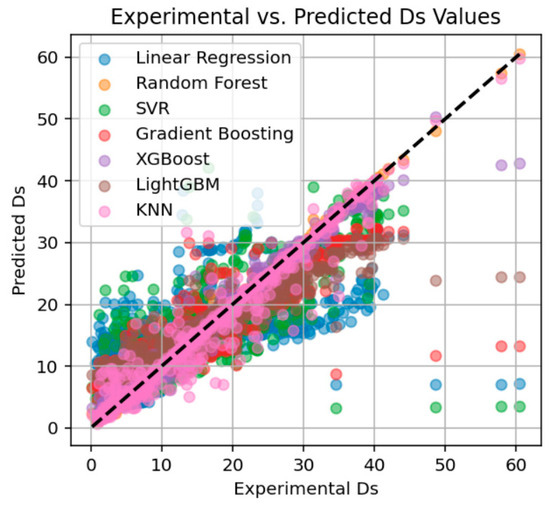
Figure 4.
The comparison between experimental and predicted values of Ds.
The Linear Regression (LR) model displays a relatively high level of dispersion, particularly at higher Ds values. This pattern indicates its limited ability to capture the nonlinear relationships in the data, leading to systematic underestimations or overestimations. In contrast, tree-based models such as Random Forest (RFR) and Gradient Boosting (GBR) perform better in the mid-range of Ds values, though they still exhibit deviations from the ideal line, especially in boundary regions. This suggests their capacity to model complex patterns more effectively than linear models, but with limitations at data extremes.
Among all models, XGBoost and LightGBM (LGBM) show the closest alignment with the 1:1 reference line across a broad range of Ds values. The point clusters for these models demonstrate high density near the diagonal, indicating strong predictive accuracy and robustness. Their gradient-boosted architecture allows them to effectively handle nonlinearities and variable interactions, making them the most reliable models in this comparative analysis.
The Support Vector Regression (SVR) model exhibits visible deviations, particularly at higher Ds values, suggesting its sensitivity to hyperparameter tuning and kernel selection. Similarly, the KNN model tends to form scattered clusters and shows inconsistent predictions across the Ds range. This behavior may result from its local approximation nature, which struggles in regions with sparse data distribution, leading to poor generalization.
Overall, proximity to the diagonal line is a visual indicator of prediction quality. When coupled with numerical performance metrics, the figure supports the conclusion that XGBoost, LightGBM, and Gradient Boosting Regression deliver superior performance for time-dependent Ds prediction tasks. These findings highlight the suitability of ensemble tree-based methods for modeling complex hydrodynamic phenomena such as equilibrium scour depth in bridge abutments.
To identify the model providing the highest similarity, the predictions of all models used were compared with the experimental data of flow depth (Y) = 9.48 cm, abutment length (L) = 10 cm, channel width (B) = 0.60 m, median grain size (d50) = 0.50 mm, flow velocity (V) = 0.64 m/s, and time (t) ranging from 0 to 973,800 s were given in Figure 5. The predictions were generated using seven distinct machine learning models: Linear Regression (LR), Random Forest (RFR), Support Vector Regression (SVR), Gradient Boosting (GBR), XGBoost, LightGBM (LGBM), and K-Nearest Neighbors (KNN).
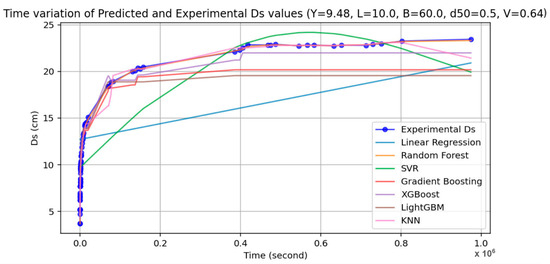
Figure 5.
Comparison of measured Ds values with predicted data.
At the initial time interval (t ≈ 0 to 100,000 s), all models exhibit a steep increase in Ds values, reflecting the rapid scouring process that typically occurs at the onset of flow conditions. Most models, particularly XGBoost, Gradient Boosting, Random Forest (RFR), and KNN, demonstrate a quick convergence toward their respective asymptotic Ds values within the first 0.1 million seconds. This stabilization suggests their effective learning of the temporal saturation behavior of scour depth.
The Linear Regression model (LR) shows a significantly different trend, exhibiting a steady and unrealistic linear increase in Ds over time. Unlike ensemble and kernel-based models, Linear Regression fails to capture the nonlinear saturation curve commonly observed in time-dependent scour processes. This underlines its structural limitation in modeling complex temporal behavior in hydraulic systems.
The Support Vector Regression model (SVR) displays a noticeably delayed increase in Ds, followed by an overshooting trend that peaks near 0.6 million seconds before declining. This nonphysical fluctuation suggests potential overfitting or sensitivity to parameter scaling and kernel configuration. Despite its theoretical capacity for nonlinear modeling, SVR appears less stable than ensemble methods in this context.
Both XGBoost and LightGBM (LGBM) show strong and consistent performance across the full-time range. Their predictions plateau at reasonable Ds levels and exhibit minimal oscillation, reflecting high generalization capability and resistance to noise. Gradient Boosting (GBR) follows a similar but slightly more rigid progression, stabilizing earlier and maintaining a nearly constant Ds afterward.
The KNN model closely mimics ensemble models during early time steps but shows minor fluctuations in the later time stages. As a non-parametric model, its behavior is heavily influenced by local sample distributions, which may explain these minor inconsistencies under sparse or shifting temporal conditions.
Overall, models such as XGBoost, LightGBM, and Gradient Boosting provide the most physically realistic and temporally stable predictions of Ds under fixed hydraulic input conditions. Their performance over time aligns well with empirical observations in sediment transport literature, suggesting their high suitability for dynamic scour depth prediction tasks. In contrast, Linear Regression and SVR display inadequate performance due to oversimplification and instability, respectively.
Figure 6 presents a comparative analysis of the prediction accuracy of seven machine learning models—Linear Regression (LR), Random Forest Regressor (RFR), Support Vector Regression (SVR), Gradient Boosting Regression (GBR), XGBoost, LightGBM (LGBM), and K-Nearest Neighbors (KNN)—used for the estimation of the time variation in scour depth (Ds). Two key error metrics are utilized: Root Mean Square Error (RMSE) and Mean Absolute Percentage Error (MAPE).
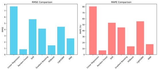
Figure 6.
Comparison of RMSE and MAPE metrics belonging to machine learning models.
In terms of RMSE (left side of Figure 6), the Linear Regression model shows the highest error, indicating a poor ability to capture the nonlinear relationships inherent in the scour process. On the other hand, Random Forest yields the lowest RMSE, followed closely by XGBoost, highlighting their superior performance in minimizing absolute prediction errors. Models such as SVR, GBR, and LightGBM exhibit moderate RMSE values, while KNN performs comparably well but with slightly higher error than the top-performing ensemble models.
The MAPE metric (right side of Figure 6), which accounts for relative prediction errors, reveals a similar trend. Random Forest again achieves the best performance, with an MAPE below 10%, followed by XGBoost and KNN. In contrast, Linear Regression exhibits the poorest result, with an MAPE exceeding 80%, underscoring its limitations in accurately estimating Ds values across a wide range. Interestingly, LightGBM, while effective in terms of RMSE, shows a relatively higher MAPE, suggesting that it may be more sensitive to errors in lower-value predictions.
Overall, as illustrated in Figure 6, ensemble-based methods, particularly Random Forest and XGBoost, consistently outperform traditional and kernel-based models in both absolute and relative error metrics. These results support their suitability for robust, data-driven modeling of time-dependent scour processes in hydraulic engineering applications.
4. Discussion
This study investigates the significant potential of machine learning (ML) models in accurately predicting the time variation in scour depth (Ds) around bridge abutments by using experimental data. Among the evaluated algorithms, ensemble-based models, particularly the Random Forest Regressor (RFR) and K-Nearest Neighbors (KNN), achieved the highest prediction accuracy, with estimations nearly identical to the experimental values.
The performance of the most successful models, RFR and KNN, is supported by SHAP and feature importance analyses. Both models identified the parameters with the strongest known physical impact on scour flow velocity (V) and abutment length (L) as the most important variables. RFR’s high performance stems from its ability to capture these complex, nonlinear physical relationships and generalize them by averaging across multiple decision trees. KNN’s success demonstrates the validity of the ‘local similarity’ assumption for this dataset, establishing that similar hydraulic conditions produce similar scour results, and shows that the model can effectively detect these similarities.
Consistency across the dataset compiled from diverse experimental sources was ensured using dimensionless parameters and a rigorous outlier removal process. This methodology eliminated scale effects and allowed the model to learn fundamental hydraulic relationships rather than absolute values. Therefore, the high accuracy achieved provides confidence that the models are learning general physical principles, not artifacts of a particular experimental setup.
As in the study, the highest similarities between experimental data and mathematical predictions were obtained in RFR metric models and gave the best results; even some predictions were very close to 100% similarity. In Figure 7, the longest experimental data of the authors, whose experimental data were used in this study, and RFR metric predictions belonging to these time variation series, were compared with each other. As seen in Figure 7, all authors’ experimental data and RFR data overlap with each other. It is also clearly seen from this figure that the more data available, the better the estimation observed.
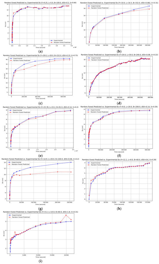
Figure 7.
Comparison of the authors’ experimental data gathered from the literature and belonging RFR model. (a) Experimental data of reference [18]. (b) Experimental data of reference [19]. (c) Experimental data of reference [20]. (d) Experimental data of reference [21]. (e) Experimental data of reference [22]. (f) Experimental data of reference [23]. (g) Experimental data of reference [24]. (h) Experimental data of reference [9]. (i) Experimental data of reference [25].
Using the reference value of 8.20 cm, as shown in Table 5, RFR predicted a Ds of 8.1890 cm, while KNN yielded 8.16 cm, confirming their robustness in modeling nonlinear and time-dependent scour processes.
The superior performance of RFR can be attributed to its ensemble architecture, which aggregates multiple decision trees trained on bootstrapped samples, thereby enhancing generalization and minimizing overfitting. Similarly, KNN’s instance-based learning approach offers flexibility in capturing local variations in the dataset, making it particularly effective in scenarios with dense, high-quality measurements. However, its sensitivity to data sparsity in certain regions suggests that careful preprocessing and distance metric selection are essential for optimal performance.
In contrast, traditional Linear Regression (LR) produced the poorest results, significantly overestimating the scour depth (11.7131 cm) and exhibiting high error rates in both absolute and relative metrics (as visualized in Figure 4, Figure 5 and Figure 6). This underperformance is consistent with its linear structure, which fails to accommodate the inherent nonlinearities of sediment transport and flow-induced scour dynamics.
Models such as XGBoost, Gradient Boosting Regressor (GBR), and LightGBM (LGBM) also demonstrated strong performance, though slightly less precise than RFR and KNN. Their gradient-based learning frameworks allow for efficient handling of complex interactions between input variables, as evidenced by their close alignment with the experimental trend in both static and time-evolving scour predictions (see Figure 6). These models provide an advantageous balance between accuracy, training speed, and interpretability, which are key considerations for real-time engineering applications.
Interestingly, while Support Vector Regression (SVR) theoretically supports nonlinear modeling through kernel transformations, its performance lagged behind that of the ensemble methods. Its overshooting behavior and instability in long-term predictions suggest potential sensitivity to hyperparameter tuning and feature scaling, which must be addressed for improved applicability.
Collectively, the visual and numerical evidence highlights that tree-based ensemble models offer superior generalization, scalability, and robustness for scour prediction tasks. Moreover, the time-dependent evaluations presented in Figure 5 reveal that models such as XGBoost and LGBM successfully capture the initial rapid scour phase and the eventual asymptotic stabilization, mimicking realistic scour behavior observed in field and laboratory studies.
These results not only validate the effectiveness of AI-driven approaches in hydraulic modeling but also emphasize their potential to replace or augment conventional empirical methods. The ability of ML models to learn from diverse datasets and capture complex nonlinear interactions offers a significant advantage for engineering design, risk mitigation, and infrastructure maintenance planning. Future research could focus on integrating hybrid architectures, such as combining physical equations with deep learning, and exploring real-time data assimilation for adaptive scour management.
This study builds upon and significantly expands the authors’ previous work on equilibrium scour depth estimation [17]. Unlike the previous work, the main innovation of this work is the estimation of scour depth over time. This is critical information for structural safety, particularly in dynamic events such as floods, where equilibrium conditions cannot be reached. Furthermore, the dataset was expanded from 150 to 3275 records, a time (t) parameter was added, and the analysis scope was expanded by incorporating new algorithms such as LightGBM (LGBM) and K-Nearest Neighbors (KNN) into the model comparison.
The findings of this study have practical implications for real-time assessment of bridge scour risk. Ensemble models such as RFR and XGBoost stand out as robust predictors that can form the basis of early warning systems due to their high accuracy and stability. For engineers, the dominant influence of flow velocity and abutment size on scour depth reaffirms the importance of prioritizing these parameters in the design phase and monitoring of existing structures.
5. Conclusions
This study presents a comprehensive evaluation of multiple machine learning algorithms for predicting the time variation in scour depth (Ds) around bridge abutments under clear-water flow conditions. Seven models Linear Regression (LR), Support Vector Regression (SVR), Random Forest Regressor (RFR), XGBoost, Gradient Boosting Regressor (GBR), LightGBM (LGBM), and K-Nearest Neighbors (KNN), were trained and tested using hydraulic and sedimentological parameters commonly encountered in engineering practice.
The results demonstrate that ensemble learning techniques, particularly RFR and KNN, yielded the most accurate predictions, closely matching the experimentally obtained scour depth. These models effectively captured the nonlinear relationships between variables and demonstrated strong generalization capabilities. Tree-based methods such as XGBoost, GBR, and LGBM also produced reliable results and successfully modeled the time-dependent scour development, while traditional linear approaches like LR exhibited limited predictive power in this nonlinear context.
The study further highlights the advantage of integrating data-driven methods into hydraulic engineering, especially for complex scour processes where empirical equations may fall short. The use of machine learning allows for improved adaptability to variable site conditions and greater predictive accuracy based on historical or real-time data.
For future research, expanding the dataset with more diverse and high-resolution experimental and field observations will enhance model robustness. Additionally, hybrid models that combine physical principles with deep learning architectures could offer even more accurate and interpretable solutions for scour prediction.
In conclusion, machine learning models, especially ensemble and instance-based algorithms, represent a powerful and promising tool for improving the reliability and safety of hydraulic infrastructure by enabling accurate, scalable, and time-sensitive scour depth estimation.
Supplementary Materials
The following supporting information can be downloaded at: https://www.mdpi.com/article/10.3390/w17172657/s1, Figure S1: Linear Regression (LR) workflow; Figure S2: Support Vector Regression (SVR) workflow; Figure S3: Random Forest Regressor (RFR) workflow; Figure S4: Gradient Boosting (GBR) workflow; Figure S5: XGBoost workflow; Figure S6: LightGBM (LGBM) workflow; Figure S7: K-Nearest Neighbors (KNN) workflow.
Author Contributions
Conceptualization, Y.U. and Ş.Y.K.; Data curation, Y.U. and Ş.Y.K.; Formal analysis, Y.U.; Investigation, Y.U. and Ş.Y.K.; Methodology, Y.U.; Supervision, Y.U.; Visualization, Y.U.; Writing—original draft, Y.U.; Writing—review and editing, Y.U. and Ş.Y.K. All authors have read and agreed to the published version of the manuscript.
Funding
This research received no external funding.
Data Availability Statement
The original contributions presented in this study are included in the article/Supplementary Material. Further inquiries can be directed to the corresponding author.
Acknowledgments
The authors are indebted to Francesco Ballio for supplying the experimental data and the Technical Research and Quality Control Laboratory of General Directorate of State Hydraulic Works for this experimental study.
Conflicts of Interest
The authors declare no conflicts of interest.
Abbreviations
The following abbreviations are used in this manuscript:
| LR | Linear Regression |
| SVR | Support Vector Regression |
| LGBM | Light Gradient Boosting Machine |
| RFR | Random Forest Regressor |
| KNN | K-Nearest Neighbors |
References
- Sui, J.; Afzalimehr, H.; Samani, A.K.; Maherani, M. Clear-Water Scour around Semi-Elliptical Abutments with Armored Beds. Int. J. Sediment Res. 2010, 25, 233–245. [Google Scholar] [CrossRef]
- Melville, B.W.; Coleman, S.E. Bridge Scour; Water Resources Publication: Littleton, CO, USA, 2000. [Google Scholar]
- Federal Highway Adminisration. Evaluating Scour at Bridges; Federal Administration: Washington, DC, USA, 2001. [Google Scholar]
- Lee, T.L.; Jeng, D.S.; Zhang, G.H.; Hong, J.H. Neural Network Modeling for Estimation of Scour Depth Around Bridge Piers. J. Hydrodyn. 2007, 19, 378–386. [Google Scholar] [CrossRef]
- Azamathulla, H.M.; Deo, M.C.; Deolalikar, P.B. Alternative Neural Networks to Estimate the Scour below Spillways. Adv. Eng. Softw. 2008, 39, 689–698. [Google Scholar] [CrossRef]
- Zounemat-Kermani, M.; Batelaan, O.; Fadaee, M.; Hinkelmann, R. Ensemble Machine Learning Paradigms in Hydrology: A Review. J. Hydrol. 2021, 598, 126266. [Google Scholar] [CrossRef]
- Hamidifar, H.; Zanganeh-Inaloo, F.; Carnacina, I. Hybrid Scour Depth Prediction Equations for Reliable Design of Bridge Piers. Water 2021, 13, 2019. [Google Scholar] [CrossRef]
- Khan, Z.U.; Khan, D.; Murtaza, N.; Pasha, G.A.; Alotaibi, S.; Rezzoug, A.; Benzougagh, B.; Khedher, K.M. Advanced Prediction Models for Scouring Around Bridge Abutments: A Comparative Study of Empirical and AI Techniques. Water 2024, 16, 3082. [Google Scholar] [CrossRef]
- Mohammadpour, R.; Ghani, A.A.; Vakili, M.; Sabzevari, T. Prediction of Temporal Scour Hazard at Bridge Abutment. Nat. Hazards 2016, 80, 1891–1911. [Google Scholar] [CrossRef]
- Choi, S.-U.; Choi, B.; Lee, S. Prediction of Local Scour around Bridge Piers Using the ANFIS Method. Neural Comput. Appl. 2017, 28, 335–344. [Google Scholar] [CrossRef]
- Hoang, N.-D.; Liao, K.-W.; Tran, X.-L. Estimation of Scour Depth at Bridges with Complex Pier Foundations Using Support Vector Regression Integrated with Feature Selection. J. Civ. Struct. Health Monit. 2018, 8, 431–442. [Google Scholar] [CrossRef]
- Abdollahpour, M.; Dalir, A.H.; Farsadizadeh, D.; Shiri, J. Assessing Heuristic Models through K-Fold Testing Approach for Estimating Scour Characteristics in Environmental Friendly Structures. ISH J. Hydraul. Eng. 2019, 25, 239–247. [Google Scholar] [CrossRef]
- Sharafati, A.; Haghbin, M.; Haji Seyed Asadollah, S.B.; Tiwari, N.K.; Al-Ansari, N.; Yaseen, Z.M. Scouring Depth Assessment Downstream of Weirs Using Hybrid Intelligence Models. Appl. Sci. 2020, 10, 3714. [Google Scholar] [CrossRef]
- Ali, A.S.A.; Günal, M. Artificial Neural Network for Estimation of Local Scour Depth Around Bridge Piers. Arch. Hydro-Eng. Environ. Mech. 2022, 68, 87–101. [Google Scholar] [CrossRef]
- Rathod, P.; Manekar, V.L. Gene Expression Programming to Predict Local Scour Using Laboratory and Field Data. ISH J. Hydraul. Eng. 2022, 28, 143–151. [Google Scholar] [CrossRef]
- Kumcu, S.Y.; Kokpinar, M.A.; Gogus, M. Scour Protection around Vertical-Wall Bridge Abutments with Collars. KSCE J. Civ. Eng. 2014, 18, 1884–1895. [Google Scholar] [CrossRef]
- Uzun, Y.; Kumcu, S.Y. Estimation of Equilibrium Scour Depth around Abutments Using Artificial Intelligence. Water 2025, 17, 1010. [Google Scholar] [CrossRef]
- Ballio, F.; Orsi, E. Time Evolution of Scour around Bridge Abutments. Water Eng. Res. 2001, 2, 243–259. [Google Scholar]
- Tey, C.B.; Raudkivi, A.J.; Melville, B.W. Local Scour at Bridge Abutments: A Report Submitted to the Roard [i.e. Road] Research Unit of the National Roads Board/by C.B. Tey; Supervised by A.J. Raudkivi and B.W. Melville. Available online: https://natlib.govt.nz/records/21454054 (accessed on 26 March 2025).
- Dongol, D.M.S.; Melville, B.W.; Zealand, T.N. Local Scour at Bridge Abutments/by Deepak Man Singh Dongol; Supervised by B.W. Melville. Available online: https://natlib.govt.nz/records/22277182 (accessed on 26 March 2025).
- Ladage, F. Temporal Development of Local Scour at Bridge Abutments; Department of Civil and Resource Engineering, University of Auckland: Auckland, New Zealand, 1998; p. 39. [Google Scholar]
- Rajaratnam, N.; Nwachukwu, B.A. Flow Near Groin-Like Structures. J. Hydraul. Eng. 1983, 109, 463–480. [Google Scholar] [CrossRef]
- Cunha, L. Time Evolution of Local Scour. In Proceedings of the 14th IAHR Congress, Paris, France, 27 July–1 August 1975. [Google Scholar]
- Oliveto, G.; Hager, W.H. Temporal Evolution of Clear-Water Pier and Abutment Scour. J. Hydraul. Eng. 2002, 128, 811–820. [Google Scholar] [CrossRef]
- Köse, Ö. A Thesis Submitted to the Graduate School of Natural and Applied Sciences of Middle East Technical University. Ph.D. Thesis, Middle East Technical University, Ankara, Turkey, 2007. [Google Scholar]
- Uzun, Y.; Saltan, F.Z. Use of Machine Learning Methods in Predicting the Main Components of Essential Oils: Laurus nobilis L. J. Essent. Oil Bear. Plants 2024, 27, 1302–1318. [Google Scholar] [CrossRef]
- Luo, M.; Liu, M.; Zhang, S.; Gao, J.; Zhang, X.; Li, R.; Lin, X.; Wang, S. Mining Soil Heavy Metal Inversion Based on Levy Flight Cauchy Gaussian Perturbation Sparrow Search Algorithm Support Vector Regression (LSSA-SVR). Ecotoxicol. Environ. Saf. 2024, 287, 117295. [Google Scholar] [CrossRef]
- Xiong, L.; An, J.; Hou, Y.; Hu, C.; Wang, H.; Chen, Y.; Tang, X. Improved Support Vector Regression Recursive Feature Elimination Based on Intragroup Representative Feature Sampling (IRFS-SVR-RFE) for Processing Correlated Gas Sensor Data. Sens. Actuators B Chem. 2024, 419, 136395. [Google Scholar] [CrossRef]
- Sánchez, J.C.M.; Mesa, H.G.A.; Espinosa, A.T.; Castilla, S.R.; Lamont, F.G. Improving Wheat Yield Prediction through Variable Selection Using Support Vector Regression, Random Forest, and Extreme Gradient Boosting. Smart Agric. Technol. 2025, 10, 100791. [Google Scholar] [CrossRef]
- Ramos Collin, B.R.; de Lima Alves Xavier, D.; Amaral, T.M.; Castro Silva, A.C.G.; dos Santos Costa, D.; Amaral, F.M.; Oliva, J.T. Random Forest Regressor Applied in Prediction of Percentages of Calibers in Mango Production. Inf. Process. Agric. 2024, 15. [Google Scholar] [CrossRef]
- EL Bilali, A.; Hadri, A.; Taleb, A.; Tanarhte, M.; EL Khalki, E.M.; Kharrou, M.H. A Novel Hybrid Modeling Approach Based on Empirical Methods, PSO, XGBoost, and Multiple GCMs for Forecasting Long-Term Reference Evapotranspiration in a Data Scarce-Area. Comput. Electron. Agric. 2025, 232, 110106. [Google Scholar] [CrossRef]
- Cheng, T.; Yao, C.; Duan, J.; He, C.; Xu, H.; Yang, W.; Yan, Q. Prediction of Active Length of Pipes and Tunnels under Normal Faulting with XGBoost Integrating a Complexity-Performance Balanced Optimization Approach. Comput. Geotech. 2025, 179, 107048. [Google Scholar] [CrossRef]
- Alsulamy, S. Predicting Construction Delay Risks in Saudi Arabian Projects: A Comparative Analysis of CatBoost, XGBoost, and LGBM. Expert Syst. Appl. 2025, 268, 126268. [Google Scholar] [CrossRef]
- Abushandi, E. Water Quality Assessment and Forecasting along the Liffey and Andarax Rivers by Artificial Neural Network Techniques Toward Sustainable Water Resources Management. Water 2025, 17, 453. [Google Scholar] [CrossRef]
- Hastie, T.; Tibshirani, R.; Friedman, J. The Elements of Statistical Learning: Data Mining, Inference, and Prediction, 2nd ed.; Springer Series in Statistics; Springer: Berlin/Heidelberg, Germany, 2009; ISBN 978-0-387-84857-0. [Google Scholar]
- Arlot, S.; Celisse, A. A Survey of Cross Validation Procedures for Model Selection. Stat. Surv. 2009, 4, 40–79. [Google Scholar] [CrossRef]
- Kohavi, R. A Study of Cross-Validation and Bootstrap for Accuracy Estimation and Model Selection. In Ijcai; Stanford University: Stanford, CA, USA, 2001; Volume 14. [Google Scholar]


Disclaimer/Publisher’s Note: The statements, opinions and data contained in all publications are solely those of the individual author(s) and contributor(s) and not of MDPI and/or the editor(s). MDPI and/or the editor(s) disclaim responsibility for any injury to people or property resulting from any ideas, methods, instructions or products referred to in the content. |
© 2025 by the authors. Licensee MDPI, Basel, Switzerland. This article is an open access article distributed under the terms and conditions of the Creative Commons Attribution (CC BY) license (https://creativecommons.org/licenses/by/4.0/).