
Turbulent Flow Through Sluice Gate and Weir Using Smoothed Particle Hydrodynamics: Evaluation of Turbulence Models, Boundary Conditions, and 3D Effects


Abstract
1. Introduction
2. Governing Equations and Solution Methodology
2.1. SPH Formulation of the Governing Equations
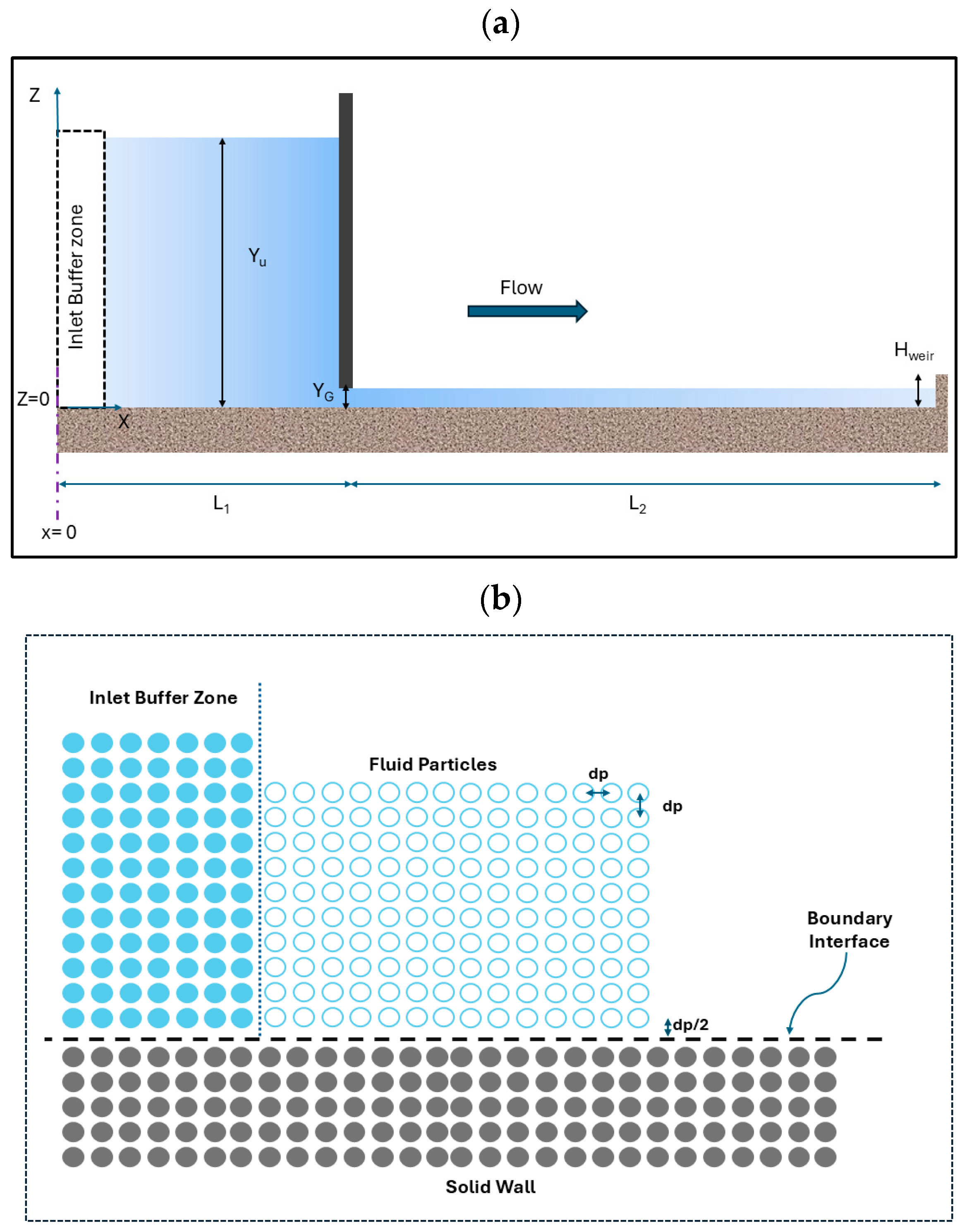
2.2. Treatment of Fluid/Solid Boundary Conditions
3. SPH Model Construction and Simulation Results
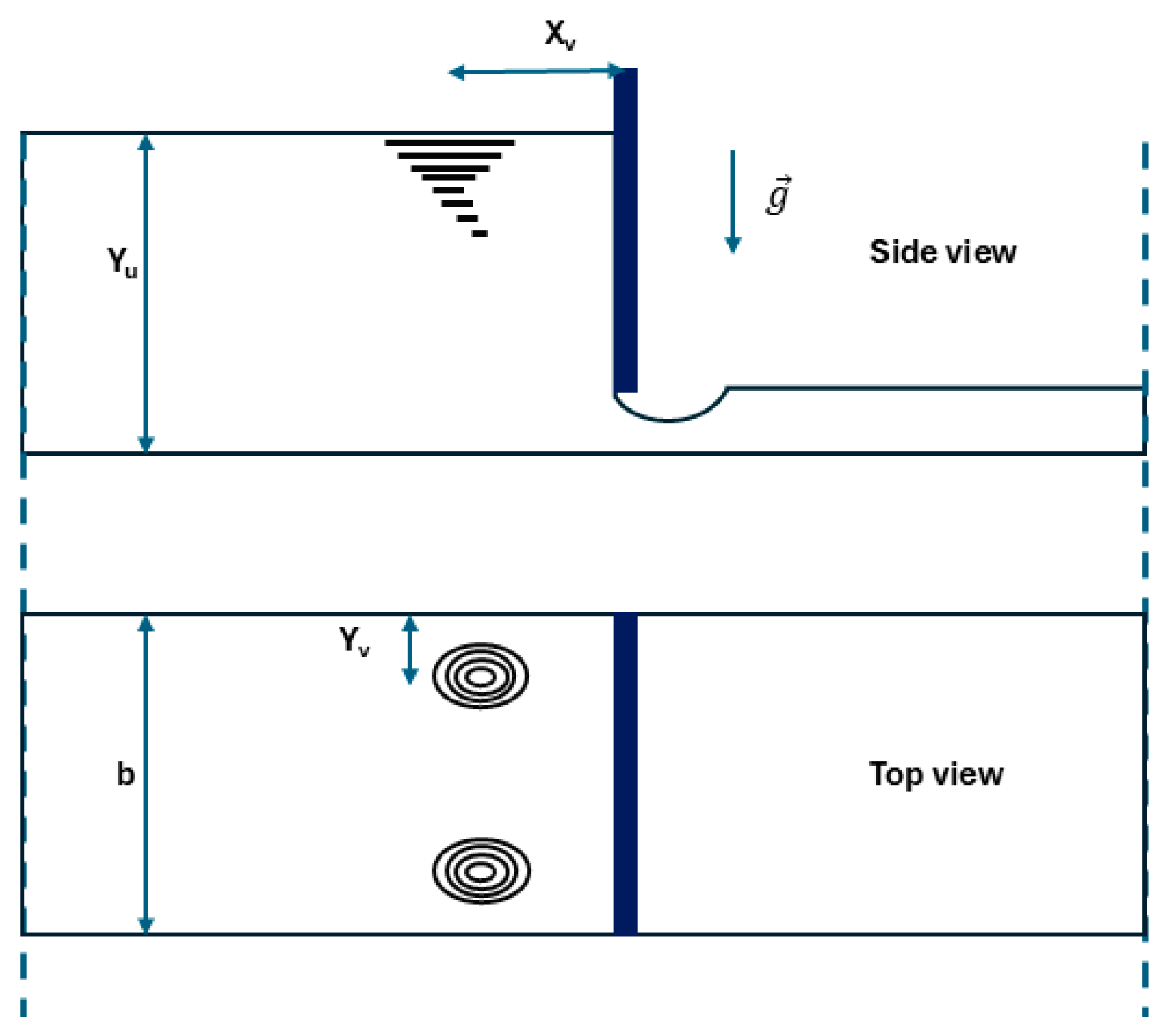
3.1. Geometry and SPH Model Construction
3.2. Physical Models
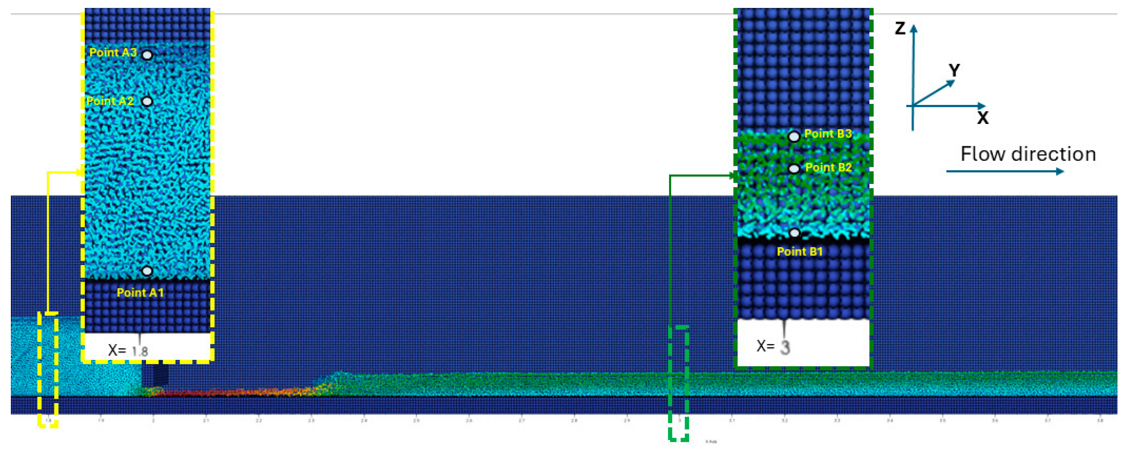
3.3. Presentation of the SPH Results
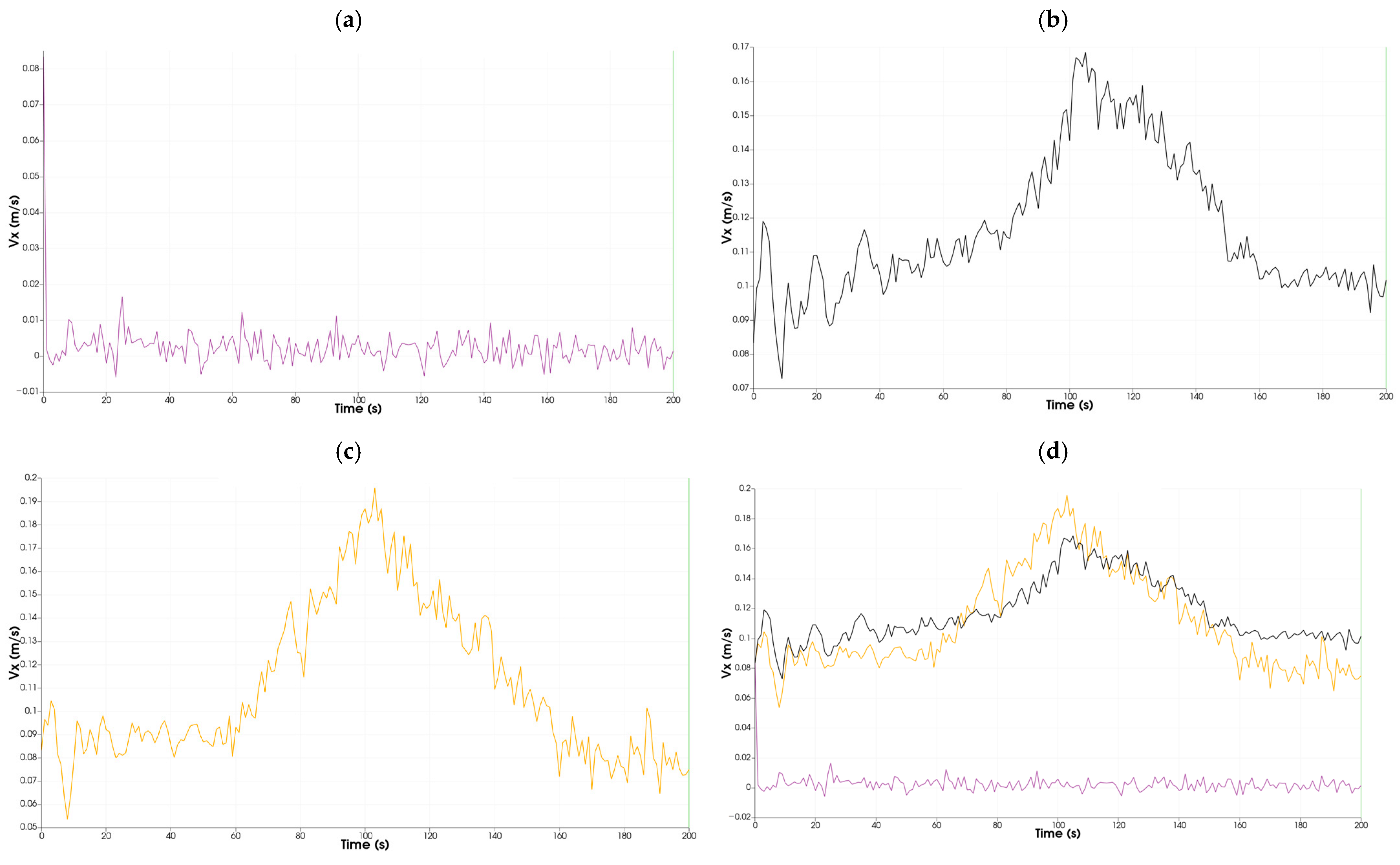
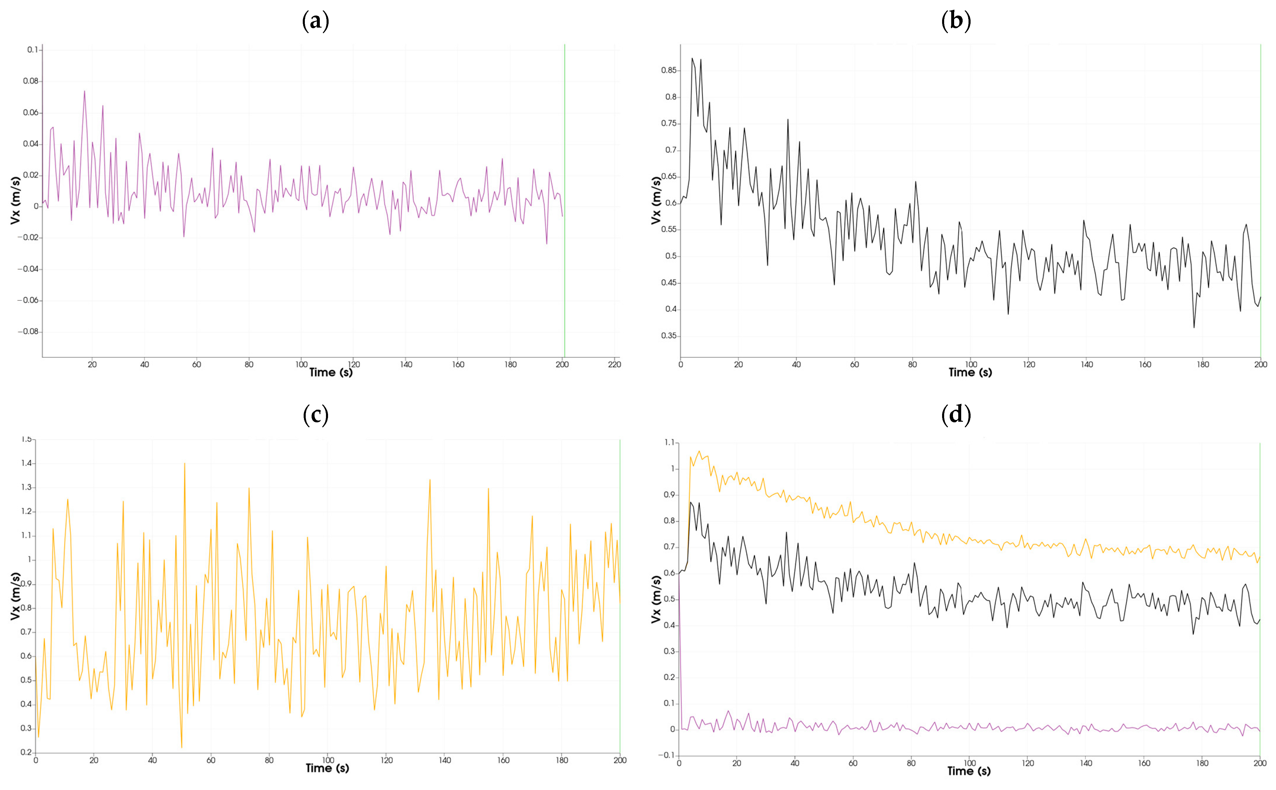
3.3.1. Artificial Viscosity Model (AVM)
3.3.2. Laminar + SPS Turbulence Model (L-SPS)
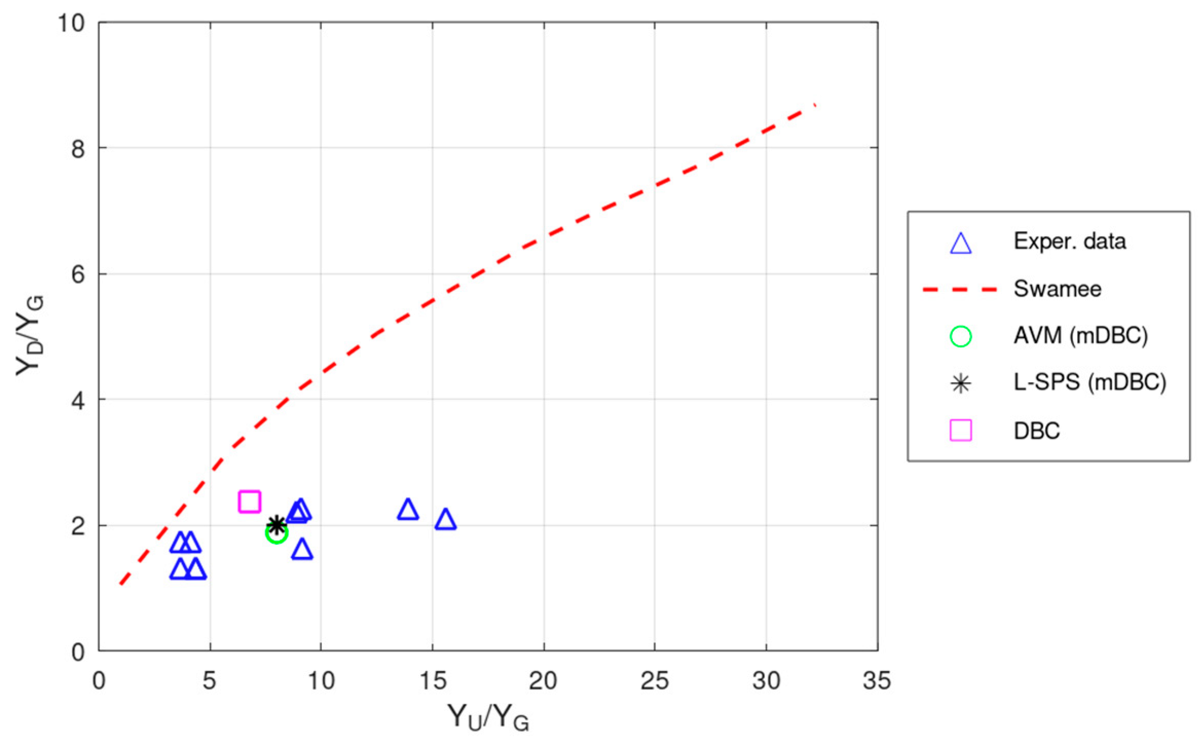
3.4. Comparison of the Present SPH Results with Yoosefdoost et al. Experimental Study
4. Discussion
5. Conclusions
Author Contributions
Funding
Data Availability Statement
Conflicts of Interest
Appendix A


Appendix B
References
- Kubrak, E.; Kubrak, J.; Kiczko, A.; Kubrak, M. Flow Measurements Using a Sluice Gate; Analysis of Applicability. Water 2020, 12, 819. [Google Scholar] [CrossRef]
- Shadloo, M.S.; Oger, G.; Le Touzé, D. Smoothed particle hydrodynamics method for fluid flows, towards industrial applications: Motivations, current state, and challenges. Comput. Fluids 2016, 136, 11–34. [Google Scholar] [CrossRef]
- Mangiardi, C.M.; Ralf, M. A hybrid algorithm for parallel molecular dynamics simulations. Comput. Phys. Commun. 2017, 219, 196–208. [Google Scholar] [CrossRef]
- Espanol, P.; Patrick, B.W. Perspective: Dissipative particle dynamics. J. Chem. Phys. 2017, 146, 150901. [Google Scholar] [CrossRef] [PubMed]
- Ellero, M.; Español, P. Everything you always wanted to know about SDPD⋆ (⋆but were afraid to ask). Appl. Math. Mech. 2017, 39, 103–124. [Google Scholar] [CrossRef]
- Gingold, R.A.; Monaghan, J.J. Smoothed particle hydrodynamics-theory and application to non-spherical stars. Mon. Not. Astron. Soc. 1977, 181, 375–389. [Google Scholar] [CrossRef]
- Violeau, D. Fluid Mechanics and the SPH Method: Theory and Applications; Oxford University Press: Oxford, UK, 2012. [Google Scholar]
- Altomare, C.; Scandura, P.; Cáceres, I.; Viccione, G. Large-scale wave breaking over a barred beach: SPH numerical simulation and comparison with experiments. Coast. Eng. 2023, 185, 104362. [Google Scholar] [CrossRef]
- Altomare, C.; Suzuki, T.; Domínguez, J.M.; Crespo, A.J.; Gómez-Gesteira, C.; Caceres, I. A hybrid numerical model for coastal engineering problems. In Proceedings of the 34th International Conference on Coastal Engineering (ICCE), Seoul, Republic of Korea, 15–20 June 2014. [Google Scholar] [CrossRef]
- Lind, S.J.; Stansby, P.K.; Rogers, B.D.; Lloyd, P.M. Numerical predictions of water-air wave slam using incompressible-compressible smoothed particle hydrodynamics. Appl. Ocean. Res. 2015, 49, 57–71. [Google Scholar] [CrossRef]
- Amaro, A.; Liang-Yee, C.; Sergei, K.B. A comparison between weakly-compressible smoothed particle hydrodynamics (WCSPH) and moving particle semi-implicit (MPS) methods for 3D dam-break flows. Int. J. Comput. Methods 2021, 18, 2050036. [Google Scholar] [CrossRef]
- Zhu, G.X.; Zou, L.; Chen, Z.; Wang, A.; Liu, M. An improved SPH model for multiphase flows with large density ratios. Int. J. Numer. Methods Fluids 2018, 86, 167–184. [Google Scholar] [CrossRef]
- Pozorski, J.; Olejnik, M. Smoothed particle hydrodynamics modelling of multiphase flows: An overview. Acta Mech. 2024, 235, 1685–1714. [Google Scholar] [CrossRef]
- Mayrhofer, A.; Laurence, D.; Rogers, B.D.; Violeau, D. DNS and LES of 3-D wall-bounded turbulence using smoothed particle hydrodynamics. Comput. Fluids 2015, 115, 86–97. [Google Scholar] [CrossRef]
- Chatzoglou, E.; Liakopoulos, A.; Sofos, F. Smoothed Particle Hydrodynamics-Based Study of 3D Confined Microflows. Fluids 2023, 8, 137. [Google Scholar] [CrossRef]
- Alexiadis, A.; Ghraybeh, S.; Qiao, G. Natural convection and solidification of phase-change materials in circular pipes: A SPH approach. Comput. Mater. Sci. 2018, 150, 475–483. [Google Scholar] [CrossRef]
- Sigalotti, L.D.; Alvarado-Rodríguez, G.; Aragón, F.; Álvarez Salazar, V.S.; Carvajal-Mariscal, I.; Real Ramirez, C.A.; Gonzalez-Trejo, J.; Klapp, J. SPH simulations and experimental investigation of water flow through a Venturi meter of rectangular cross-section. Sci. Rep. 2023, 13, 21215. [Google Scholar] [CrossRef] [PubMed]
- Chatzoglou, E.; Liakopoulos, A. Flow regimes in sluice gate-weir systems: 3D SPH-based model validation. In Proceedings of the 17th International SPHERIC Workshop, Rhodes, Greece, 27–29 June 2023. [Google Scholar]
- Zhang, J.; Wang, B.; Jiang, Q.; Hou, G.; Li, Z.; Liu, H. Numerical Study of Fluid–Solid Interaction in Elastic Sluice Based on SPH Method. Water 2023, 15, 3738. [Google Scholar] [CrossRef]
- Martínez-Estévez, I.; Tagliafierro, B.; El Rahi, J.; Domínguez, J.M.; Crespo, A.J.; Troch, P.; Gómez-Gesteira, M. Coupling an SPH-based solver with an FEA structural solver to simulate free surface flows interacting with flexible structures. Comput. Methods Appl. Mech. Eng. 2023, 410, 115989. [Google Scholar] [CrossRef]
- Vacondio, R.; Altomare, C.; De Leffe, M.; Hu, X.; Le Touzé, D.; Lind, S.; Souto-Iglesias, A. Grand challenges for smoothed particle hydrodynamics numerical schemes. Comput. Part. Mech. 2021, 8, 575–588. [Google Scholar] [CrossRef]
- Monaghan, J.J. Simulating free surface flows with SPH. J. Comput. Phys. 1994, 110, 399–406. [Google Scholar] [CrossRef]
- Monaghan, J.J.; Kajtar, J.B. SPH particle boundary forces for arbitrary boundaries. Comput. Phys. Commun. 2009, 180, 1811–1820. [Google Scholar] [CrossRef]
- Kulasegaram, S.; Bonet, J.; Lewis, R.W.; Profit, M. A variational formulation based contact algorithm for rigid boundaries in twodimensional SPH applications. Comput. Mech. 2004, 33, 316–325. [Google Scholar] [CrossRef]
- Leroy, A.; Violeau, D.; Ferrand, M.; Kassiotis, C. Unified semianalytical wall boundary conditions applied to 2-D incompressible SPH. J. Comput. Phys. 2014, 261, 106–129. [Google Scholar] [CrossRef]
- Mayrhofer, A.; Rogers, B.D.; Violeau, D.; Ferrand, M. Investigation of wall bounded flows using SPH and the unified semi-analytical wall boundary conditions. Comput. Phys. Commun. 2013, 184, 2515–2527. [Google Scholar] [CrossRef]
- Crespo, A.J.C.; Gomez-Gesteira, M.; Dalrymple, R.A. Boundary conditions generated by dynamic particles in SPH methods. Comput. Mater. Contin. 2007, 5, 173–184. [Google Scholar] [CrossRef]
- Marrone, S.; Antuono MA, G.D.; Colagrossi, A.; Colicchio, G.; Le Touzé, D.; Graziani, G. δ-SPH model for simulating violent impact flows. Comput. Methods Appl. Mech. Eng. 2011, 200, 1526–1542. [Google Scholar] [CrossRef]
- Adami, S.; Hu, X.Y.; Adams, N.A. A generalized wall boundary condition for smoothed particle hydrodynamics. J. Comput. Phys. 2012, 231, 7057–7075. [Google Scholar] [CrossRef]
- Fourtakas, G.; Dominguez, J.M.; Vacondio, R.; Rogers, B.D. Local uniform stencil (LUST) boundary condition for arbitrary 3-D boundaries in parallel smoothed particle hydrodynamics (SPH) models. Comput. Fluids 2019, 190, 346–361. [Google Scholar] [CrossRef]
- English, A.; Domínguez, J.M.; Vacondio, R.; Crespo, A.J.C.; Stansby, P.K.; Lind, S.J.; Gómez-Gesteira, M. Modified dynamic boundary conditions (mDBC) for general-purpose smoothed particle hydrodynamics (SPH): Application to tank sloshing, dam break and fish pass problems. Comput. Part. Mech. 2022, 9, 1–15. [Google Scholar] [CrossRef]
- Yoosefdoost, M.; Lubitz, W.D. Sluice gate design and calibration: Simplified models to distinguish flow conditions and estimate discharge coefficient and flow rate. Water 2022, 14, 1215. [Google Scholar] [CrossRef]
- Domínguez, J.M.; Fourtakas, G.; Altomare, C.; Canelas, R.B.; Tafuni, A.; García-Feal, O.; Martínez-Estévez, I.; Mokos, A.; Vacondio, R.; Crespo, A.J.C.; et al. DualSPHysics: From fluid dynamics to multiphysics problems. Comput. Part. Mech. 2022, 9, 867–895. [Google Scholar] [CrossRef]
- Monaghan, J.J. Smoothed particle hydrodynamics. Annu. Rev. Astron. Astrophys. 1992, 30, 543–574. [Google Scholar] [CrossRef]
- Liu, G.R. Mesh Free Methods: Moving Beyond the Finite Element Method; CRC Press: Boca Raton, FL, USA, 2003. [Google Scholar]
- Monaghan, J.J. Smoothed Particle Hydrodynamics. Rep. Prog. Phys. 2005, 68, 1703–1759. [Google Scholar] [CrossRef]
- Wendland, H. Piecewiese polynomial, positive definite and compactly supported radial functions of minimal degree. Adv. Comput. Math. 1995, 4, 389–396. [Google Scholar] [CrossRef]
- Altomare, C.; Crespo, A.J.; Domínguez, J.M.; Gómez-Gesteira, M.; Suzuki, T.; Verwaest, T. Applicability of Smoothed Particle Hydrodynamics for estimation of sea wave impact on coastal structures. Coast. Eng. 2015, 96, 1–12. [Google Scholar] [CrossRef]
- Dalrymple, R.A.; Rogers, B.D. Numerical modeling of water waves with the SPH method. Coast. Eng. 2006, 53, 141–147. [Google Scholar] [CrossRef]
- Tafuni, A.; Dominguez, J.M.; Vacondio, R.; Crespo, A.J.C. A versatile algorithm for the treatment of open boundary conditions in Smoothed particle hydrodynamics GPU models. Comput. Methods Appl. Mech. Eng. 2018, 342, 604–624. [Google Scholar] [CrossRef]
- Liu, M.B.; Liu, G.R. Restoring particle consistency in smoothed particle hydrodynamics. Appl. Numer. Math. 2006, 56, 19–36. [Google Scholar] [CrossRef]
- Roth, A.; Hager, W.H. Underflow of standard sluice gate. Exp. Fluids 1999, 27, 339–350. [Google Scholar] [CrossRef]
- Chaudhry, M. Open-Channel Flow; Prentice-Hall: Englewood Cliffs, NJ, USA, 1993. [Google Scholar]
- Liakopoulos, A. Hydraulics, 3rd ed.; Tziolas Publications: Thessaloniki, Greece, 2020. [Google Scholar]
- Basa, M.; Quinlan, N.J.; Lastiwka, M. Robustness and accuracy of SPH formulations for viscous flow. Int. J. Numer. Methods Fluids 2009, 60, 1127–1148. [Google Scholar] [CrossRef]
- Swamee, P. Sluice-Gate Discharge Equations. J. Irrig. Drain. Eng. 1992, 118, 56–60. [Google Scholar] [CrossRef]
- Dalrymple, A.; Knio, O. SPH modelling of water waves. Coast. Dyn. 2001, 1, 779–787. [Google Scholar]
- Liu, S.; Ioan, N.; Majid, M. Evaluation of the solid boundary treatment methods in SPH. Int. J. Ocean Coast. Eng. 2018, 1, 1840002. [Google Scholar] [CrossRef]
- Gotoh, H.; Shao, S.; Memita, T. SPH-LES model for numerical investigation of wave interaction with partially immersed breakwater. Coast. Eng. J. 2001, 46, 39–63. [Google Scholar] [CrossRef]
- Chatzoglou, E.; Liakopoulos, A. Hydraulic jump simulation via Smoothed Particle Hydrodynamics: A critical review. In Proceedings of the 39th IAHR World Congress, Granada, Spain, 19–24 June 2022. [Google Scholar]
- Liakopoulos, A. Computation of high speed turbulent boundary-layer flows using The k-ε turbulence model. Int. J. Numer. Methods Fluids 1985, 5, 81–97. [Google Scholar] [CrossRef]
- Sahan, R.A.; Albin, D.C.; Sahan, N.K.; Liakopoulos, A. Artificial Neural Network-Based Low-Order Dynamical Modeling and Intelligent Control of Transitional Flow Systems. In Proceedings of the Sixth IEEE Conference on Control Applications, Hartford, CT, USA, 5–7 October 1997. [Google Scholar]


| Case | YG (m) | YU (m) | Hweir (m) | Np | Density (kg/m3) | Physical Model | Simulation Time (s) |
|---|---|---|---|---|---|---|---|
| AVM | 0.025 | 0.20 | 0.025 | 2057327 | 1000 | Artificial visc. | 200 |
| L-SPS | 0.025 | 0.20 | 0.025 | 2057327 | 1000 | Laminar + SPS | 200 |
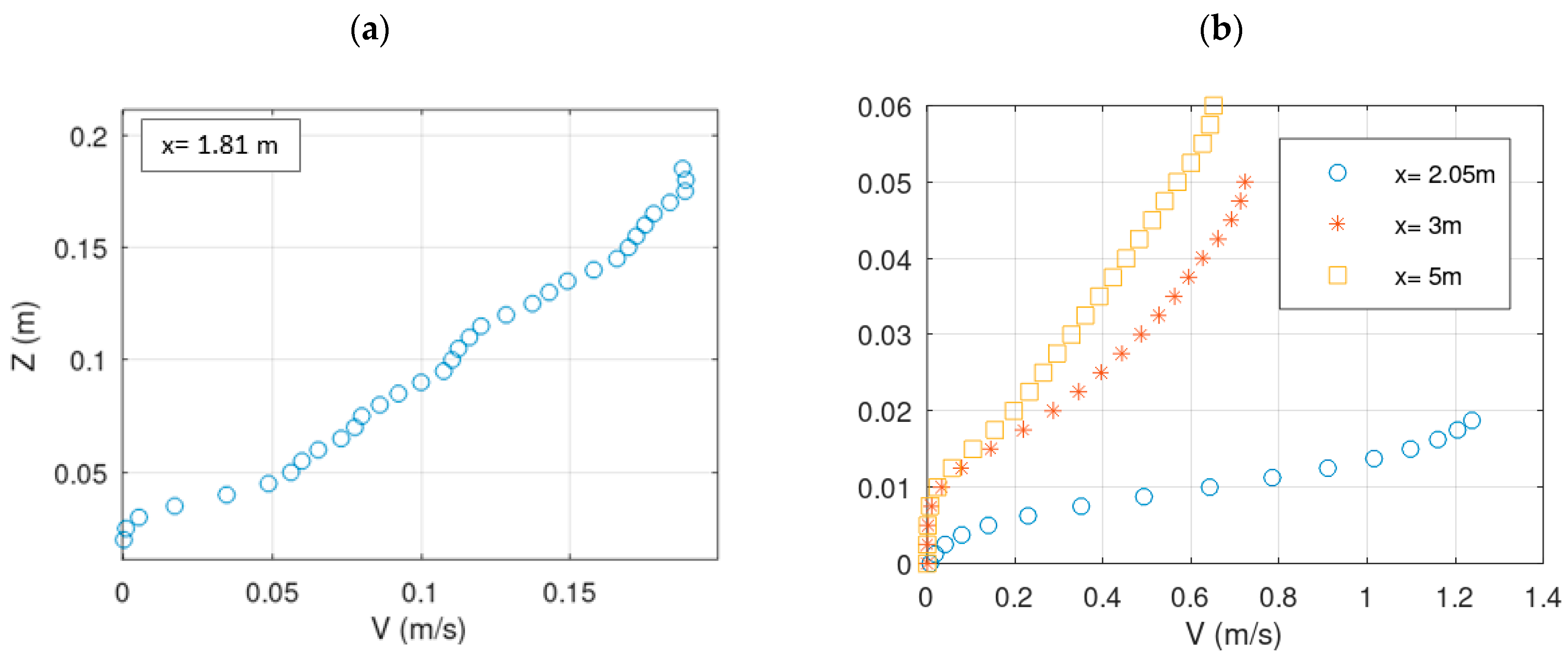
| V1_81 = 0.093 m/s | V2_05 = 0.9 m/s | V3 = 0.336 m/s |
| h1_81 = 0.18 m | h2_05 = 0.0187 m | h3 = 0.05 m |
| q1_81 = 0.0168 m2/s | q2_05 = 0.0168 m2/s | q3 = 0.0168 m2/s |
| V1_81 = 0.093 m/s | V2_05 = 0.96 m/s | V3 = 0.335 m/s |
| h1_81 = 0.18 m | h2_05 = 0.0175 m | h5 = 0.05 m |
| q1_81 = 0.0168 m2/s | q2_05 = 0.0168 m2/s | q3 = 0.0168 m2/s |
Disclaimer/Publisher’s Note: The statements, opinions and data contained in all publications are solely those of the individual author(s) and contributor(s) and not of MDPI and/or the editor(s). MDPI and/or the editor(s) disclaim responsibility for any injury to people or property resulting from any ideas, methods, instructions or products referred to in the content. |
© 2025 by the authors. Licensee MDPI, Basel, Switzerland. This article is an open access article distributed under the terms and conditions of the Creative Commons Attribution (CC BY) license (https://creativecommons.org/licenses/by/4.0/).
Share and Cite
Chatzoglou, E.; Liakopoulos, A. Turbulent Flow Through Sluice Gate and Weir Using Smoothed Particle Hydrodynamics: Evaluation of Turbulence Models, Boundary Conditions, and 3D Effects. Water 2025, 17, 152. https://doi.org/10.3390/w17020152
Chatzoglou E, Liakopoulos A. Turbulent Flow Through Sluice Gate and Weir Using Smoothed Particle Hydrodynamics: Evaluation of Turbulence Models, Boundary Conditions, and 3D Effects. Water. 2025; 17(2):152. https://doi.org/10.3390/w17020152
Chicago/Turabian StyleChatzoglou, Efstathios, and Antonios Liakopoulos. 2025. "Turbulent Flow Through Sluice Gate and Weir Using Smoothed Particle Hydrodynamics: Evaluation of Turbulence Models, Boundary Conditions, and 3D Effects" Water 17, no. 2: 152. https://doi.org/10.3390/w17020152
APA StyleChatzoglou, E., & Liakopoulos, A. (2025). Turbulent Flow Through Sluice Gate and Weir Using Smoothed Particle Hydrodynamics: Evaluation of Turbulence Models, Boundary Conditions, and 3D Effects. Water, 17(2), 152. https://doi.org/10.3390/w17020152