When Are Models Useful? Revisiting the Quantification of Reality Checks

Abstract

The Nash–Sutcliffe efficiency remains the best metric for measuring the appropriateness of a model and reflects a culture developed in hydrology to test models against reality before using them. This metric is not without problems, and alternative metrics have been proposed subsequently. Here, the concept of knowable moments is exploited to provide robust metrics that assess not only the second-order properties of the process of interest but also high-order moments which provide information for the entire distribution function of the process of interest. This information may be useful in hydrological tasks, as most hydrological processes are non-Gaussian. The proposed concepts are illustrated, also in relationship to existing ones, using a large-scale comparison of climatic model outputs for precipitation with reality for the last 84 years on hemispheric and continental scales.

                                                                                                                                                                                  All models are wrong but some are useful

(George E. P. Box) [1]

1. Introduction

The aphorism in the epigram is very popular and expresses the fact that models are only approximations of reality. The first part of the aphorism, “all models are wrong”, is wrong per se in a rigorous epistemological context. The meaning it purports to express could perhaps be better formulated as “models differ from reality”. They differ not only in quantitative terms, e.g., when a real value is six units and a model predicts five units. Even if a model gives a value identical to the real one (e.g., six units), again it differs from reality conceptually as the model is a representation (usually mathematical, simplifying and approximate) of reality, not the physical reality per se [2]. The model differs from the system it represents even in the case that the latter is a hardware and/or software implementation of an algorithm [3]. In an era where confusion has prevailed over rigor, it is essential to clarify the conceptual difference between models and reality, which makes a model not “wrong” or “right” but different conceptually from reality.

The second part of the aphorism, “some [models] are useful”, is not problematic and is the subject of this paper. The usefulness of a model needs modeling per se. In other words, the usefulness needs to be quantified by metrics that describe how good the quantified approximation of reality is. This quantification is typically based on simulation results by the model and comparison with observations. The comparison typically uses statistical or stochastic concepts such as variances and correlation coefficients. This implies that we have to take an additional modeling step, i.e., to assume that both model simulation outputs, $s$, and actual observations, $x$, are further represented as stochastic variables (or even stochastic processes), $\underset{\_}{s},\underset{\_}{x}$ (notice the notational convention to underline stochastic variables). This step may not be necessary if the model is deterministic, yet taking it allows us to use the advanced language and tools of stochastics, which facilitates modeling.

Standard statistical metrics of this type are the correlation coefficient, $r_{\underset{\_}{s}\underset{\_}{x}}$, between $\underset{\_}{s}$ and $\underset{\_}{x}$, and its square, $r_{\underset{\_}{s}\underset{\_}{x}}^2$, known as the coefficient of determination. These, however, do not provide a holistic picture of the similarity between $\underset{\_}{s}$ and $\underset{\_}{x}$ as they do not reflect the similarity (or otherwise) of the marginal distribution. For example, $\underset{\_}{s}$ and $\underset{\_}{x}$ may have a large $r_{\underset{\_}{s}\underset{\_}{x}}$, suggesting good model performance, and simultaneously a large difference in their means, suggesting poor performance because of bias.

The most common metric of a holistic type has been the Nash–Sutcliffe efficiency (NSE). It was proposed by two famous hydrologists, Nash and Sutcliffe (1970) [4], in a study that for a long time has been the most cited hydrological paper [5] (currently about 28,000 citations in Google Scholar and more than 18,000 in Scopus). Its use has been common beyond hydrology, such as in geophysics, earth sciences, atmospheric sciences, environmental sciences, statistics, engineering, data science, and computational intelligence, e.g., [6,7,8,9,10,11,12,13,14,15,16,17]. As noted by O’Connell et al. [18], the discipline of hydrology has commonly been an “importer” of ideas, techniques, and theories developed in other scientific disciplines. A rare exception is Hurst’s work [19], which was “exported” to many areas of science and technology. The model performance metric proposed by Nash and Sutcliffe (NSE) is another rare exception of “exportation”.

A different metric that has recently attracted wide attention in hydrology and beyond is the Kling–Gupta efficiency (KGE) proposed by the hydrologists Kling and Gupta [20,21]. Both metrics, NSE and KGE, are expressed in terms of the first- and second-order classical moments of the variables $\underset{\_}{s},\underset{\_}{x}$ or their difference, i.e., the error $\underset{\_}{e}$. Both are dimensionless and have an upper bound, the number 1, which corresponds to the perfect agreement of simulated with observed values. However, they have differences. NSE has a conceptual and rigorous definition based on the expectation of the squared error. KGE is a rather arbitrary expression, heuristically combining three indices of agreement. These also appear in NSE if it is decomposed using stochastic algebra. It is useful that the KGE metric distinguishes the three separate indicators of agreement, but it is doubtful if their combination in one metric is useful.

Both NSE and KGE provide useful information for processes that are Gaussian or close to Gaussian but, as will be shown in the analyses that follow, fail to perform in processes with behavior far different from Gaussian. On the other hand, most real-world processes differ from Gaussian. In non-Gaussian processes, a single criterion of a model’s efficiency may not suffice, and multiple criteria are needed, of which a selection could be made depending on the users’ needs. For example, in hydrology, forecasting low flows or floods requires good agreement between modeled and observed discharges across wide ranges. Therefore, we need some metrics that can (a) provide useful information for non-Gaussian processes, and especially for the behavior at the distribution tails, and (b) can offer multiple options that serve different user requirements. Non-Gaussianity, focus on distribution tails, and a multiplicity of options require information that can hardly be extracted from second-order statistical properties. On the other hand, high-order moments are unknowable if the information is extracted from the data [22,23,24,25,26]. Yet, the new concept of knowable moments or K-moments [23,24,25,26] can, on the one hand, replace the classical second-order moments and, on the other hand, extend the definition of metrics for high orders.

This is attempted in this study, after re-examining the NSE and KGE metrics, which are based on classical moments, and locating their strengths and weaknesses (Section 2). An alternative framework based on K-moments is proposed, and some synthetic examples are used to illustrate the properties of both the existing and the proposed frameworks (Section 3). In addition, an application to real-world processes, namely the precipitation process, is presented, where the real system is assumed to be described by reanalysis data for precipitation, while the models are assumed to be some popular climate models (Section 4).

2. Revisiting the Existing Framework

2.1. Nash–Sutcliffe Efficiency

The error between the simulated and actual processes is defined as

$$\underset{\_}{e} :=\underset{\_}{s}-\underset{\_}{x}$$

(1)

Based on this, the Nash–Sutcliffe efficiency is defined as

$$\mathrm{NSE} :=1-{\displaystyle \frac{\mathrm{E}\left[{\underset{\_}{e}}^2\right]}{\mathrm{var}\left[\underset{\_}{x}\right]}}$$

(2)

The error can be decomposed as

$$\mathrm{E}\left[{\underset{\_}{e}}^2\right]=\mathrm{var}\left[\underset{\_}{e}\right]+\mathrm{E}{\left[\underset{\_}{e}\right]}^2={\sigma }_{\underset{\_}{e}}^2+{\mu }_{\underset{\_}{e}}^2$$

(3)

with ${\sigma }_{\underset{\_}{e}}^2 :=\mathrm{var}\left[\underset{\_}{e}\right],{\mu }_{\underset{\_}{e}}:=\mathrm{E}\left[\underset{\_}{e}\right]$. Hence, the NSE can be decomposed as

$$\mathrm{NSE}=\mathrm{EV}-{\mathrm{RB}}^2$$

(4)

where EV and RB are the explained variance and the relative bias, respectively:

$$\mathrm{EV}=1-{\displaystyle \frac{{\sigma }_{\underset{\_}{e}}^2}{{\sigma }_{\underset{\_}{x}}^2}}, \mathrm{RB} :={\displaystyle \frac{{\mu }_{\underset{\_}{e}}}{{\sigma }_{\underset{\_}{x}}}}={\displaystyle \frac{{\mu }_{\underset{\_}{s}}-{\mu }_{\underset{\_}{x}}}{{\sigma }_{\underset{\_}{x}}}}$$

(5)

Alternatively, in the decomposition, we can substitute the statistics of $\underset{\_}{s}$ for those of $\underset{\_}{e}$ and find

$$\mathrm{E}\left[{\underset{\_}{e}}^2\right]={\sigma }_{\underset{\_}{s}}^2+{\sigma }_{\underset{\_}{x}}^2-2r_{\underset{\_}{s}\underset{\_}{x}}{\sigma }_{\underset{\_}{s}}{\sigma }_{\underset{\_}{x}}+{\mu }_{\underset{\_}{e}}^2$$

(6)

Hence,

$$\mathrm{EV}=2r_{\underset{\_}{s}\underset{\_}{x}}{\displaystyle \frac{{\sigma }_{\underset{\_}{s}}}{{\sigma }_{\underset{\_}{x}}}}-{\displaystyle \frac{{\sigma }_{\underset{\_}{s}}^2}{{\sigma }_{\underset{\_}{x}}^2}}, \mathrm{NSE}=2r_{\underset{\_}{s}\underset{\_}{x}}{\displaystyle \frac{{\sigma }_{\underset{\_}{s}}}{{\sigma }_{\underset{\_}{x}}}}-{\displaystyle \frac{{\sigma }_{\underset{\_}{s}}^2}{{\sigma }_{\underset{\_}{x}}^2}}-{\left({\displaystyle \frac{{\mu }_{\underset{\_}{s}}-{\mu }_{\underset{\_}{x}}}{{\sigma }_{\underset{\_}{x}}}}\right)}^2$$

(7)

It follows directly that, when ${\mu }_{\underset{\_}{s}}={\mu }_{\underset{\_}{x}}$, the metrics $\mathrm{EV}=\mathrm{NSE}$ are maximized for

$${\sigma }_{\underset{\_}{s}}=\left\{\begin{array}{cc}{r}_{\underset{\_}{s}\underset{\_}{x}}{\sigma }_{\underset{\_}{x}},& r_{\underset{\_}{s}\underset{\_}{x}}\ge 0\\ 0,& r_{\underset{\_}{s}\underset{\_}{x}}\le 0\end{array}\right.$$

(8)

and their maximum value is

$${\mathrm{EV}}_{\max }={\mathrm{NSE}}_{\max }=\left\{\begin{array}{cc}{r}_{\underset{\_}{s}\underset{\_}{x}}^2,& r_{\underset{\_}{s}\underset{\_}{x}}\ge 0\\ 0,& r_{\underset{\_}{s}\underset{\_}{x}}\le 0\end{array}\right.$$

(9)

Notably, the maximum value is not achieved when ${\sigma }_{\underset{\_}{s}}={\sigma }_{\underset{\_}{x}}$. Rather, the value that corresponds to the latter case is

$$\mathrm{EV}=\mathrm{NSE}=2r_{\underset{\_}{s}\underset{\_}{x}}-1\le r_{\underset{\_}{s}\underset{\_}{x}}^2$$

(10)

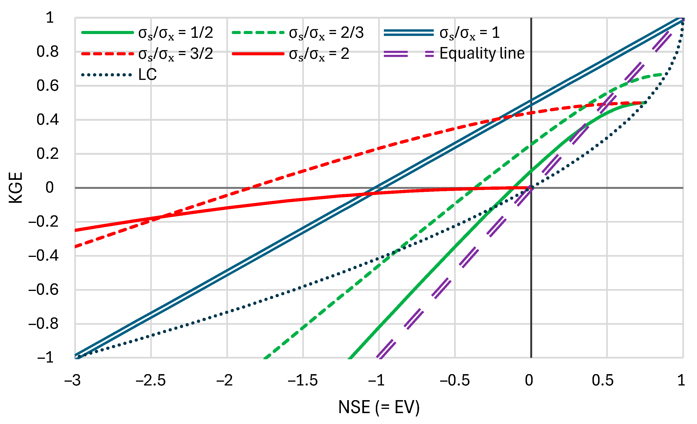
2.2. Kling–Gupta Efficiency and Its Relationship with the Nash–Sutcliffe Efficiency

The Kling–Gupta efficiency is defined as

$$\mathrm{KGE}=1-\sqrt{{\left(1-r_{\underset{\_}{s}\underset{\_}{x}}\right)}^2+{\left(1-{\displaystyle \frac{{\sigma }_{\underset{\_}{s}}}{{\sigma }_{\underset{\_}{x}}}}\right)}^2+{\left(1-{\displaystyle \frac{{\mu }_{\underset{\_}{s}}}{{\mu }_{\underset{\_}{x}}}}\right)}^2}$$

(11)

The definition is heuristic, and thus KGE does not represent a formal statistic. The last term is pathological as it is often the case that ${\mu }_{\underset{\_}{x}}=0$ (e.g., when departures from the mean, usually called “anomalies”, are modeled), in which KGE becomes $-\infty$. If we exclude the pathological last term, KGE becomes equivalent, but not equal, to EV in the sense that both express second-order properties.

For fixed $r_{\underset{\_}{s}\underset{\_}{x}}$, the maximum value of KGE is achieved for ${\mu }_{\underset{\_}{s}}={\mu }_{\underset{\_}{x}},{\sigma }_{\underset{\_}{s}}={\sigma }_{\underset{\_}{x}}$ and is

$${\mathrm{KGE}}_{\max }=r_{\underset{\_}{s}\underset{\_}{x}}$$

(12)

For ${\mu }_{\underset{\_}{s}}={\mu }_{\underset{\_}{x}},{\sigma }_{\underset{\_}{s}}\ne {\sigma }_{\underset{\_}{x}}$, after algebraic operations, we find that KGE and EV are related by

$$\mathrm{KGE}=1-\sqrt{{\left(1-{\displaystyle \frac{\mathrm{EV}+{\sigma }_{\underset{\_}{s}}^2/{\sigma }_{\underset{\_}{x}}^2}{2{\sigma }_{\underset{\_}{s}}/{\sigma }_{\underset{\_}{x}}}}\right)}^2+{\left(1-{\displaystyle \frac{{\sigma }_{\underset{\_}{s}}}{{\sigma }_{\underset{\_}{x}}}}\right)}^2}$$

(13)

In the limiting case that $r_{\underset{\_}{s}\underset{\_}{x}}=1$ (and ${\mu }_s={\mu }_x$), we find

$$\mathrm{KGE}={\displaystyle \frac{{\sigma }_{\underset{\_}{s}}}{{\sigma }_{\underset{\_}{x}}}}, \mathrm{EV}=2{\displaystyle \frac{{\sigma }_{\underset{\_}{s}}}{{\sigma }_{\underset{\_}{x}}}}-{\displaystyle \frac{{\sigma }_{\underset{\_}{s}}^2}{{\sigma }_{\underset{\_}{x}}^2}}=2\mathrm{KGE}-{\mathrm{KGE}}^2\iff \mathrm{KGE}=1-\sqrt{1-\mathrm{EV}}$$

(14)

Equations (13) and (14) are illustrated in Figure 1, where it can be seen that (a) when the explained variance EV = NSE is high, say > 0.5, the value of KGE is smaller than EV; (b) when EV = NSE is 0, the value of KGE can be as high as 0.5 (for ${\sigma }_{\underset{\_}{s}}/{\sigma }_{\underset{\_}{x}}=1)$; (c) when the EV is negative, the KGE value is less negative; (d) in general, KGE tends to decrease, in absolute value, the effectiveness metric that is provided by the EV = NSE; (e) this is further verified from the curve corresponding to ${\sigma }_{\underset{\_}{s}}/{\sigma }_{\underset{\_}{x}}$, which has a slope of 1/2 instead of 1. In brief, KGE is a less sensitive metric than NSE.

All in all, the heuristic character, the smaller sensitivity, and the problematic division by the mean, which can be zero, do not favor the use of KGE, and thus it will not be used in this paper. A substitute with some mathematical meaning, namely the absolute error efficiency (AEE) (rather than the squared error in NSE), is the following, computed in Appendix A:

$$\mathrm{AEE}\approx 1-\sqrt{{\left(1-{\displaystyle \frac{{\sigma }_{\underset{\_}{s}}}{{\sigma }_{\underset{\_}{x}}}}\right)}^2+2{\displaystyle \frac{{\sigma }_{\underset{\_}{s}}}{{\sigma }_{\underset{\_}{x}}}}\left(1-r_{\underset{\_}{s}\underset{\_}{x}}\right)+{\displaystyle \frac{\mathrm{\pi }}{2}}{\left({\displaystyle \frac{{\mu }_{\underset{\_}{s}}-{\mu }_{\underset{\_}{x}}}{{\sigma }_{\underset{\_}{x}}}}\right)}^2}$$

(15)

Notice that the quantity $\left(1-r_{\underset{\_}{s}\underset{\_}{x}}\right)$ is not squared, as it is in KGE; actually, squaring is not necessary from a mathematical point of view as it is always non-negative. Assuming that ${\mu }_{\underset{\_}{s}}={\mu }_{\underset{\_}{x}},{\sigma }_{\underset{\_}{s}}={\sigma }_{\underset{\_}{x}}$, the resulting AEE is $1-\sqrt{2\left(1-r_{\underset{\_}{s}\underset{\_}{x}}\right)}$, which takes a zero value for $r_{\underset{\_}{s}\underset{\_}{x}}=0.5$. Like in the NSE case, when ${\mu }_{\underset{\_}{s}}={\mu }_{\underset{\_}{x}}$, $\mathrm{AEE}$ is maximized with respect to ${\sigma }_{\underset{\_}{s}}$ not when ${\sigma }_{\underset{\_}{s}}={\sigma }_{\underset{\_}{x}}$ but when ${\sigma }_{\underset{\_}{s}}$ satisfies Equation (8).

3. Proposed Framework

3.1. A Summary of K-Moments

The methodologies discussed in Section 2 are based on first- and second-order distributional properties, while the framework of classical moments cannot serve the estimation of higher-order moments [22,23,26]. However, the concept of knowable moments or K-moments [23,24,25,26] can work for high-order moments.

The K-moments are defined as follows. We consider a sample of a stochastic variable $\underset{\_}{x}$, i.e., a number $p$ of independent copies of the stochastic variable $\underset{\_}{x}$, i.e., ${\underset{\_}{x}}_1,{\underset{\_}{x}}_2, \dots , {\underset{\_}{x}}_p$. If we arrange the variables in ascending order, the ith smallest, denoted as ${\underset{\_}{x}}_{\left(i:p\right)}, i=1,\dots ,p$ is termed the ith order statistic. The largest (pth) order statistic is

$${\underset{\_}{x}}_{\left(p\right)} :={\underset{\_}{x}}_{\left(p:p\right)}=\max \left({\underset{\_}{x}}_1,{\underset{\_}{x}}_2, \dots , {\underset{\_}{x}}_p\right)$$

(16)

and the smallest (first) is

$${\underset{\_}{x}}_{\left(1:p\right)}=\min \left({\underset{\_}{x}}_1,{\underset{\_}{x}}_2, \dots , {\underset{\_}{x}}_p\right)$$

(17)

Now, we define the upper knowable moment (K-moment) of order p as the expectation of the largest of the p variables ${\underset{\_}{x}}_{\left(p\right)}$:

$$K_p^{\prime } :=\mathrm{E}\left[{\underset{\_}{x}}_{\left(p\right)}\right]=\mathrm{E}\left[\max \left({\underset{\_}{x}}_1,{\underset{\_}{x}}_2, \dots , {\underset{\_}{x}}_p\right)\right]$$

(18)

where $\mathrm{E}\left[ \right]$ denotes expectation, and the lower knowable moment (K-moment) of order p as the expectation of the smallest of the p variables ${\underset{\_}{x}}_{\left(1:p\right)}$:

$${\overline{K}}_p^{\prime } :=\mathrm{E}\left[{\underset{\_}{x}}_{\left(1:p\right)}\right]=\mathrm{E}\left[\min \left({\underset{\_}{x}}_1,{\underset{\_}{x}}_2, \dots , {\underset{\_}{x}}_p\right)\right]$$

(19)

An important property, directly resulting from their definition, is that the K-moments are ordered as follows:

$${\overline{K}}_p^{\prime }\le \cdots \le {\overline{K}}_2^{\prime }\le {\overline{K}}_1^{\prime }=K_1^{\prime }=\mu \le K_2^{\prime }\le \cdots \le K_p^{\prime }$$

(20)

These moments are noncentral, and we can also define central moments as

$$K_p :=K_p^{\prime }-K_1^{\prime }, {\overline{K}}_p :={\overline{K}}_1^{\prime }-{\overline{K}}_p^{\prime }, K_p,{\overline{K}}_p\ge 0$$

(21)

As shown in [26] (chapter 6), for a stochastic variable $\underset{\_}{x}$ of continuous type, the upper K-moment of order p of $\underset{\_}{x}$ is theoretically calculated as follows:

$$K_p^{\prime }=p\mathrm{E}\left[{\left(F\left(\underset{\_}{x}\right)\right)}^{p-1}\underset{\_}{x}\right]=p\underset{-\infty }{\overset{\infty }{{\displaystyle \int }}}{\left(F\left(x\right)\right)}^{p-1}x f\left(x\right)\mathrm{d}x=p\underset{0}{\overset{1}{{\displaystyle \int }}}x\left(F\right)F^{p-1}\mathrm{d}F$$

(22)

Likewise, the lower K-moment of order p is theoretically calculated as follows:

$${\overline{K}}_p^{\prime }=p\mathrm{E}\left[{\left(\overline{F}\left(\underset{\_}{x}\right)\right)}^{p-1}\underset{\_}{x}\right]=p\underset{-\infty }{\overset{\infty }{{\displaystyle \int }}}{\left(\overline{F}\left(x\right)\right)}^{p-1}x f\left(x\right)\mathrm{d}x=p\underset{0}{\overset{1}{{\displaystyle \int }}}x\left(\overline{F}\right){\overline{F}}^{p-1}\mathrm{d}F$$

(23)

In these equations, $F\left(x\right)$ is the distribution function of $\underset{\_}{x}$, $\overline{F}\left(x\right) :=1-F\left(x\right)$ is its tail function, and $f\left(x\right) :=\mathrm{d}F\left(x\right)/\mathrm{d}x$ is its probability density function. Equations (22) and (23) allow for the extension of the evaluation of K-moments for non-integer order $p$ for a stochastic variable $\underset{\_}{x}$ of continuous type. For discrete-type variables as well as for generalizations of K-moments, the interested reader is referred to [25,26].

The unbiased estimator of the upper K-moment ${\underset{\_}{K}}_p^{\prime }$ from a sample of size $n$ is

$${\underset{¯}{\widehat{K}}}_p^{\prime }={\displaystyle \sum }_{i=1}^n{b}_{inp} {\underset{\_}{x}}_{\left(i:n\right)}$$

(24)

and that of the lower K-moment is

$${\widehat{\overline{\underset{\_}{K}}}}_p^{\prime }={\displaystyle \sum }_{i=1}^n{b}_{inp} {\underset{\_}{x}}_{\left(n-i+1:n\right)}={\displaystyle \sum }_{i=1}^n{b}_{n-i+1,n,p} {\underset{\_}{x}}_{\left(i:n\right)}$$

(25)

where

$$b_{inp}=\left\{\begin{array}{ll}0,\hfill & i<p\hfill \\ p{\displaystyle \frac{\Gamma \left(n-p+1\right)}{\Gamma \left(n+1\right)}} {\displaystyle \frac{\Gamma \left(i\right)}{\Gamma \left(i-p+1\right)}},\hfill & i\ge p\ge 0\hfill \end{array}\right.$$

(26)

and $\Gamma \left( \right)$ is the gamma function. For integer moment order $p$ and $i\ge p\ge 0$, this simplifies to

$$b_{inp}=\left(\begin{array}{c}i-1\\ p-1\end{array}\right){\displaystyle /}\left(\begin{array}{c}n\\ p\end{array}\right)$$

(27)

Based on the K-moments, we define the location (or central tendency) parameter of order $p$, $C_p$, the dispersion parameter of order $p$, $D_p$, and the (dimensionless) central-tendency-to-dispersion ratio of order $p$, $R_p$, as follows:

$$C_p :={\displaystyle \frac{K_p^{\prime }+{\overline{K}}_p^{\prime }}{2}}, D_p :={\displaystyle \frac{K_p^{\prime }-{\overline{K}}_p^{\prime }}{2}}, R_p :={\displaystyle \frac{C_p}{D_p}}={\displaystyle \frac{K_p^{\prime }+{\overline{K}}_p^{\prime }}{K_p^{\prime }-{\overline{K}}_p^{\prime }}}$$

(28)

where $D_p\ge 0$. The least-order meaningful values thereof are

$$C_1=K_1^{\prime }={\overline{K}}_1^{\prime }=\mu , D_2={\displaystyle \frac{K_2^{\prime }-{\overline{K}}_2^{\prime }}{2}}=K_2={\overline{K}}_2, R_2={\displaystyle \frac{K_1^{\prime }}{K_2}}={\displaystyle \frac{{\overline{K}}_1^{\prime }}{{\overline{K}}_2}}$$

(29)

Note that as $D_1=0, R_1=\infty .$ Also, as ${\overline{K}}_2^{\prime }=2K_1^{\prime }-K_2^{\prime }$ [26], we have $C_2=\left(1/2\right) \left(K_2^{\prime }+{\overline{K}}_2^{\prime }\right)=K_1^{\prime }=C_1$, i.e., the first- and second-order central tendency parameters are equal to each other and equal to the mean. Hence, the central-tendency-to-dispersion ratio of order 2, $R_2$, is the mean, standardized by the dispersion parameter of order 2, and is therefore similar to the quantity $\mu /\sigma$ used in classical statistics.

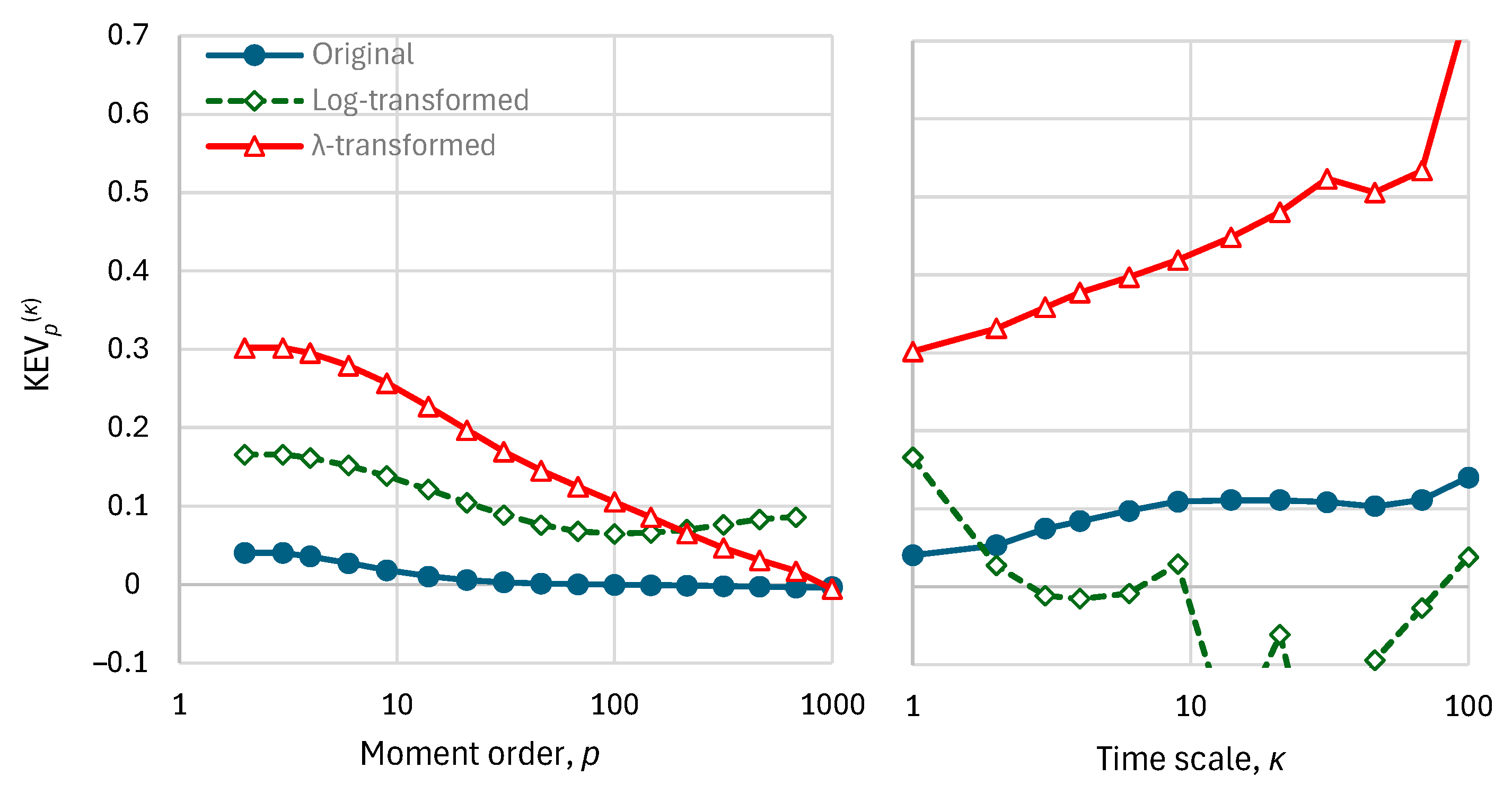
3.2. K-Moments Based Metrics of Efficiency

A perfect model will have all central tendency and dispersion parameters of the error $\underset{\_}{e}$ equal to zero: $C_p\left[\underset{\_}{e}\right]=D_p\left[\underset{\_}{e}\right]=0$ for any $p$. A good model will have nonzero but not large values. Based on the dispersion parameters, $D_p$, we can define quantities analogous to the explained variance. We define the K-unexplained variation of order $p$ and its difference from 1; the K-explained variation of order $p$ is as follows:

$${\mathrm{KUV}}_p={\displaystyle \frac{D_p\left[\underset{\_}{e}\right]}{D_p\left[\underset{\_}{x}\right]}}={\displaystyle \frac{K_p^{\prime }\left[\underset{\_}{e}\right]-{\overline{K}}_p^{\prime }\left[\underset{\_}{e}\right]}{K_p^{\prime }\left[\underset{\_}{x}\right]-{\overline{K}}_p^{\prime }\left[\underset{\_}{x}\right]}}, {\mathrm{KEV}}_p=1-{\mathrm{KUV}}_p=1-{\displaystyle \frac{D_p\left[\underset{\_}{e}\right]}{D_p\left[\underset{\_}{x}\right]}}$$

(30)

Their least-order meaningful values are

$${\mathrm{KUV}}_2={\displaystyle \frac{D_2\left[\underset{\_}{e}\right]}{D_2\left[\underset{\_}{x}\right]}}={\displaystyle \frac{K_2^{\prime }\left[\underset{\_}{e}\right]-{\overline{K}}_2^{\prime }\left[\underset{\_}{e}\right]}{K_2^{\prime }\left[\underset{\_}{x}\right]-{\overline{K}}_2^{\prime }\left[\underset{\_}{x}\right]}}={\displaystyle \frac{K_2\left[\underset{\_}{e}\right]}{K_2\left[\underset{\_}{x}\right]}}, {\mathrm{KEV}}_2=1-{\mathrm{KUV}}_2=1-{\displaystyle \frac{K_2\left[\underset{\_}{e}\right]}{K_2\left[\underset{\_}{x}\right]}}$$

(31)

The minimum and maximum possible values are, respectively, ${\mathrm{KUV}}_p=0$ and ${\mathrm{KEV}}_p=1$ and correspond to $D_p\left[\underset{\_}{e}\right]=0$. For a model that equates any $s$ with a mean of $\underset{\_}{x}$, $K_p\left[\underset{\_}{e}\right]=K_p\left[\underset{\_}{x}\right]$ for any $p\ge 2$ and ${\mathrm{KUV}}_p=1, {\mathrm{KEV}}_p=0$. Models worse than that have ${\mathrm{KUV}}_p$ higher than 1 and negative values of ${\mathrm{KEV}}_p$.

For a normal distribution, $K_2\left[\underset{\_}{e}\right]/K_2\left[\underset{\_}{x}\right]={\sigma }_{\underset{\_}{e}}/{\sigma }_{\underset{\_}{x}}$ and hence the K-moments-based metrics are related to the classical explained variance by

$${\mathrm{KUV}}_2=\sqrt{1-\mathrm{EV}}, {\mathrm{KEV}}_2=1-\sqrt{1-\mathrm{EV}}$$

(32)

Remembering that for $r_{\underset{\_}{s}\underset{\_}{x}}=1$, $\mathrm{KGE}=1-\sqrt{1-\mathrm{EV}}$ (see Figure 1), we notice the identity of ${\mathrm{KEV}}_2$ and $\mathrm{KGE}$ (as functions of EV) for this case and further observe that Equation (32) holds for any $r_{\underset{\_}{s}\underset{\_}{x}}$ for normal distribution, while that for KGE only holds for $r_{\underset{\_}{s}\underset{\_}{x}}=1$.

The bias is a separate characteristic, and it would be better dealt with based on a different statistic. The ratio $R_p$ is an appropriate metric for it. Alternatively, and in an analogous manner to ${\mathrm{KUV}}_p$, we can define the K-bias of order p as

$${\mathrm{KB}}_p={\displaystyle \frac{K_p^{\prime }\left[\underset{\_}{e}\right]+{\overline{K}}_p^{\prime }\left[\underset{\_}{e}\right]}{K_p^{\prime }\left[\underset{\_}{x}\right]-{\overline{K}}_p^{\prime }\left[\underset{\_}{x}\right]}}$$

(33)

with a special case for $p=2$

$${\mathrm{KB}}_2={\displaystyle \frac{K_2^{\prime }\left[\underset{\_}{e}\right]+{\overline{K}}_2^{\prime }\left[\underset{\_}{e}\right]}{K_2^{\prime }\left[\underset{\_}{x}\right]-{\overline{K}}_2^{\prime }\left[\underset{\_}{x}\right]}}={\displaystyle \frac{K_1^{\prime }\left[\underset{\_}{e}\right]}{K_2\left[\underset{\_}{x}\right]}}$$

(34)

It appears more natural for the two quantities describing dispersion and bias to be thought of as small as possible in order for a model to be regarded as good. To fulfil this desideratum, the metrics of choice would be the ${\mathrm{KUV}}_p$ and ${\mathrm{KB}}_p$. However, as the aim of this paper is to provide metrics with behaviour similar to the existing ones, in what follows we use ${\mathrm{KEV}}_p$ rather than the more intuitive ${\mathrm{KUV}}_p$. When the unexplained variation and bias are to be combined, a relevant expression, called the K-moment-based absolute error efficiency and derived in Appendix A, is as follows:

$$\mathrm{KAEE}\approx 1-\sqrt{{\left({\displaystyle \frac{K_2\left[\underset{\_}{e}\right]}{K_2\left[\underset{\_}{x}\right]}}\right)}^2+{\displaystyle \frac{1}{2}}{\left({\displaystyle \frac{K_1^{\prime }\left[\underset{\_}{e}\right]}{K_2\left[\underset{\_}{x}\right]}}\right)}^2}=1-\sqrt{{\mathrm{KUV}}_2^2+{\displaystyle \frac{1}{2}}{\mathrm{KB}}_2^2}$$

(35)

3.3. Possible Transformations of Data

Figure 2 (upper) compares two synthetic time series consisting of 1000 data values, an original $x_i$, and a simulated $s_i$. These synthetic series were constructed as follows. First, a series $v_i$ was generated from the Hurst–Kolmogorov model [26] with a Hurst parameter of 0.95 and normal distribution N(0,1). Then, the series $v_i$ was smoothed by a linear filter with a triangular shape with a peak value of 1 and values equal to 0 at times 10 and 20 time steps before and after the time of the peak, respectively, thus producing a series $y_i$. Subsequently, a series $z_i$ was generated by adding to $y_i$ a series $u_i$ again generated from the Hurst–Kolmogorov model with a Hurst parameter of 0.95 and normal distribution N(0,$\sqrt{2}{\sigma }_y$), where ${\sigma }_y$ is the standard deviation of $y_i$. Finally, the two latter series were exponentiated, $x_i=\exp (a{z}_i-{\mu }_z),s_i=\exp (a{y}_i-{\mu }_y)$, with $a=0.3$, and taken as original and simulated series after rounding to one decimal point. Both $x_i$ and $s_i$ exhibit long-range dependence and are log-normally distributed. The former is rough, due to the component $u_i$, while the latter is smooth.

From the visual depiction of Figure 2 (upper), it turns out that the model performance is very poor. This is also reflected in all performance metrics (see Table 2, first row, below). However, the poor performance is mostly due to the log-normal distribution of $x_i$, which yields frequent high peaks. The simulated series $s_i$ does not capture these peaks. If we take the logarithmic transformations of both $x_i$ and $s_i$, then, as seen in Figure 2 (middle), there is some resemblance of the original to simulated series, which is also reflected in the metrics for the log-transformed series (see Table 2 below).

Is a model that has this behavior, i.e., very poor performance in original values but very improved performance in transformed values, useless? An affirmative reply to this question is justified as the end-user is ultimately concerned with the original values and the model agreement with them. The reply supported here is different: a model that in a transformed space performs well is not useless. Undoubtedly, the metrics for the original series are important, but the metrics for a transformed space also have some value, given the general setting of this study, according to which multiple criteria and metrics are useful to consider.

The logarithmic transformation on which Figure 2 (middle) is based may not be appropriate for all cases and also has a problem, namely the fact that it diverges to minus infinity when the original value is zero. In our example, due to the rounding of the original and simulated values to one decimal point, 24% of the points have at least one of the two coordinates equal to zero; these were removed in the depictions (Figure 2, middle) and in the calculations (see Table 2 below).

A proper transformation that remedies these problems, by being general and free of ad hoc considerations, is the following [26] (Section 2.10), which we denote as the lambda (λ) transformation:

$$x_i^{*} :=\lambda \ln \left(1+x_i/\lambda \right)$$

(36)

and likewise for $s_i$. For low values of $x_i\ll \lambda$, including $x_i=0$, this maps $x_i$ to itself, while for large $x_i$, it maps it to a linear function of $\ln x_i$. Parameter λ is assumed to be the same for both $x_i$ and $s_i$. We can estimate it numerically by maximizing one of the model efficiency metrics.

To illustrate the features of this transformation, we use the following example, noting that the original values in Figure 2 (middle) span four orders of magnitude from 0.1 to 1000, something that would not happen if the distribution were normal but happens quite often if the distribution is log-normal, as in our example (and even more so if the distribution is heavy tailed, e.g., Pareto). The illustration is provided in

Table 1. Illustration of the different distances (metrics for error).

#	$\mathit{x}, \mathit{s}$	Euclidean Distance	Logarithmic Distance	λ Distance for λ = 1
1	$x$ = 0$, s$ = 0.1	0.1 − 0 = 0.1	ln 0.1 − ln 0 = ∞	ln 1.1 − ln 1 = 0.10
2	$x$ = 0.1$, s$ = 0.2	0.2 − 0.1 = 0.1	ln 0.2 − ln 0.1 = 0.69	ln 1.2 − ln 1.1 = 0.09
3	$x$ = 100$, s$ = 100.1	100.1 − 100 = 0.1	ln 100.1 − ln 100 = 0.001	ln 101.1 − ln 101 = 0.001
4	$x$ = 100$, s$ = 110	110 − 100 = 10	ln 110 − ln 100 = 0.10	ln 111 − ln 101 = 0.09
5	$x$ = 100$, s$ = 200	200 − 100 = 100	ln 200 − ln 100 = 0.69	ln 201 − ln 101 = 0.69

for five cases (#1–#5) of different couples of $\left(x,s\right)$. One would assert that the first two cases #1 and #2 ($x=0, s=0.1$ and $x=0.1, s=0.2$) reflect good model performance with an error of 0.1 only, if measured by the Euclidean distance or by the λ distance. However, if the logarithmic distance is used, these errors are very high, even ∞ in the former case. Now, if the actual value is $x=100$, and we wish to tell which of the cases #3–#5 ($s=100.1, 110, 200$) is as good as #2 ($x=0.1, s=0.2$), the answer depends on the distance metric used. According to the Euclidean distance, the answer would be $s$ = 100.1, while according to the logarithmic distance, it would be as high as $s$ = 200. The λ distance with $\lambda =1$ gives an intermediate reply, $s$ = 110. From a practical point of view, the latter looks reasonable: a distance of 10, corresponding to a 10% error, when $x=100$ is equally good as a distance of 0.1 when $x$ = 0.1; it would be too strict to demand a distance of 0.1 when $x=100$.

It is noted that in hydrology, the Box–Cox transformation ($x_i^{**} :=\left(x_i^a-1\right)/a$ for $a>0$, reducing to the logarithmic transformation, $x_i^{**}=\ln x_i$, when $a=0$) has been more common than the above λ transformation. However, this is not appropriate for the task being discussed as it does not behave differently for different ranges of the variable. By choosing $a=1$ and $a=0$, we precisely recover the Euclidean and logarithmic distances, respectively, but either of these behaviors apply to the entire range of the variable.

Adopting the λ transformation, we may give it some more degrees of freedom for the simulated series. Specifically, unless the model is physically based and its simulation results have some physical meaning, we may use the additional parameters α and β to adapt the transformation as follows:

$$s_i^{**}:=\alpha +\beta \lambda \ln \left(1+s_i/\lambda \right)$$

(37)

with default values $\alpha =0, \beta =1$. Again, these are obtained by optimization together with the optimization of $\lambda$, noting that $\lambda$ applies to both $x_i$ and $s_i$, but α and β apply to $s_i$ only.

Table 2. Model efficiency metrics and fitted parameters of transformations for the example depicted on Figure 2.

Site	λ	α	β	r	EV	RB	NSE	KGE	KEV2	KB2	AEE
Untransformed				0.364	0.049	−0.167	0.022	−0.371	0.040	−0.921	−0.160
Log-transformed				0.571	0.299	−0.179	0.277	0.398	0.165	−0.315	0.136
λ-transformed	0.044	0	1	0.708	0.486	−0.131	0.477	0.656	0.292	−0.233	0.273
λ-transformed	0.024	−0.005	1.057	0.714	0.504	−0.019	0.504	0.649	0.302	−0.033	0.301

gives the optimized values of $\lambda$ for our example and for the default values of α and β, as well as the optimized values of all three parameters, and the resulting optimal metrics of model efficiency. Figure 2 (lower) shows the transformed time series $x_i^{*}$ and $s_i^{**}$, where a good agreement between the two is seen, in contrast to the upper panel of the same figure.

Figure 2. An example illustrating a case in which the poor performance of a model improves substantially after transformation of the variables: (upper) original series on a decimal plot; (middle) original series on a logarithmic plot; and (lower) λ-transformed series with parameters shown in Table 2 (last row).

Figure 2. An example illustrating a case in which the poor performance of a model improves substantially after transformation of the variables: (upper) original series on a decimal plot; (middle) original series on a logarithmic plot; and (lower) λ-transformed series with parameters shown in Table 2 (last row).

The metrics optimized for the two λ-transformed series of Table 2 are the KEV₂ when the default values $\alpha =0,\beta =1$ are used and the KAEE otherwise. These are not the only options as high-order metrics could also have been chosen to be optimized. The higher-order metrics when the KEV₂ is optimized are shown in Figure 3 (left), also in comparison to those of the untransformed and the logarithmically transformed series. As seen in the figure, the performance deteriorates with the increase in the moment order.

Figure 3 does not give any information about the model bias. This is provided in Figure 4 in terms of both the ratio $R_p$ and the K-bias ${\mathrm{KB}}_p$. As seen in the graphs, both indices practically provide the same information, and there is no substantial variation in the bias metrics with order p. However, the λ transformation reduces the bias of the original series substantially.

With the above methodology, we may find increased performance measures in cases that the range of the variable spans several orders of magnitude. The increase cannot be arbitrary but has an upper bound, determined by optimization. If the distribution is normal, or close to it, no increase at all is expected.

It should be noted that there are cases on the contrary, where the standard metrics are artificially inflated and need to be reduced. Specifically, when processes have a periodic component (as most hydrological processes have at a sub-annual scale), then capturing the periodicity alone results in high performance metrics, even if the model is fully unable to simulate the deviations from the periodic signal. Again, we may deal with this issue using a transformation. In this case, the common transformation is the standardization of the time series, ${\tilde{x}}_{\tau }=\left(x_{\tau }-{\mu }_{\tau }\right)/{\sigma }_{\tau }$, where the mean ${\mu }_{\tau }$ and the standard deviation ${\sigma }_{\tau }$ are periodic functions of time $\tau$. Examples of this technique can be seen in Koutsoyiannis et al. [27] (their Table 1), where the NSE of some modes is as high as 0.85 for the original series but become negative after standardization by monthly means and standard deviations.

An additional transformation which may be useful in assessing the usefulness of models is the change in the time scale. A model may be poor in, say, a fine time scale, but when aggregated to a coarser scale, its performance may improve (or vice versa). Therefore, it may be useful to assess the model in multiple time scales. The change from time scale 1 ($x_{\tau })$ to time scale $\kappa$ ($x_{\tau }^{\left(\kappa \right)}$) is easily made by averaging the time series, i.e., $x_{\tau }^{\left(\kappa \right)} :=\left(x_{\left(\tau -1\right)\kappa +1}+\dots +x_{\tau \kappa }\right)/\kappa$ (and likewise for $s_{\tau }^{\left(\kappa \right)}$). An example is shown in Figure 3 (right) (for the time series of Figure 2), which shows that the performance improves in terms of the KEV₂ metric, when the time scale increases.

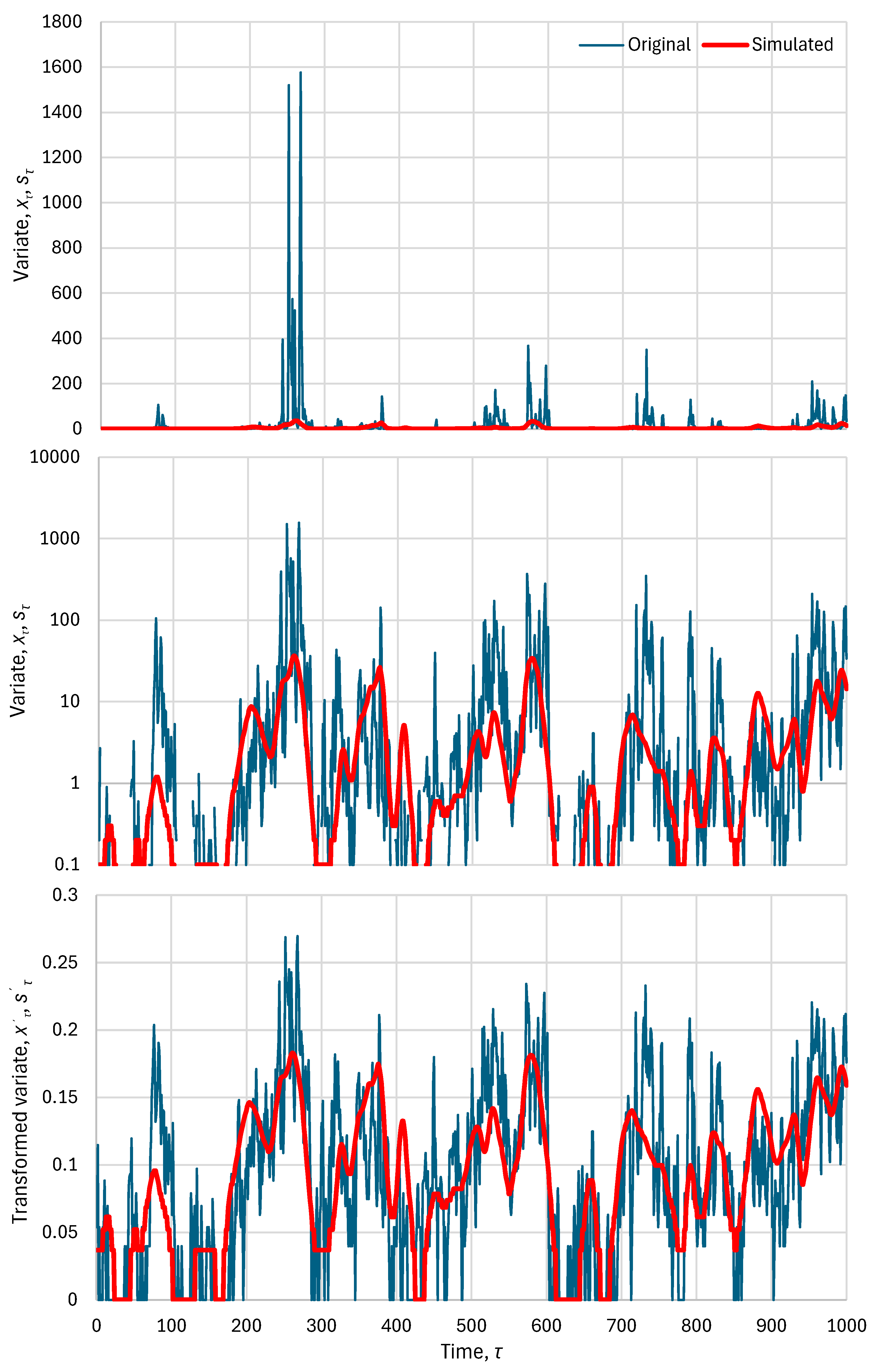
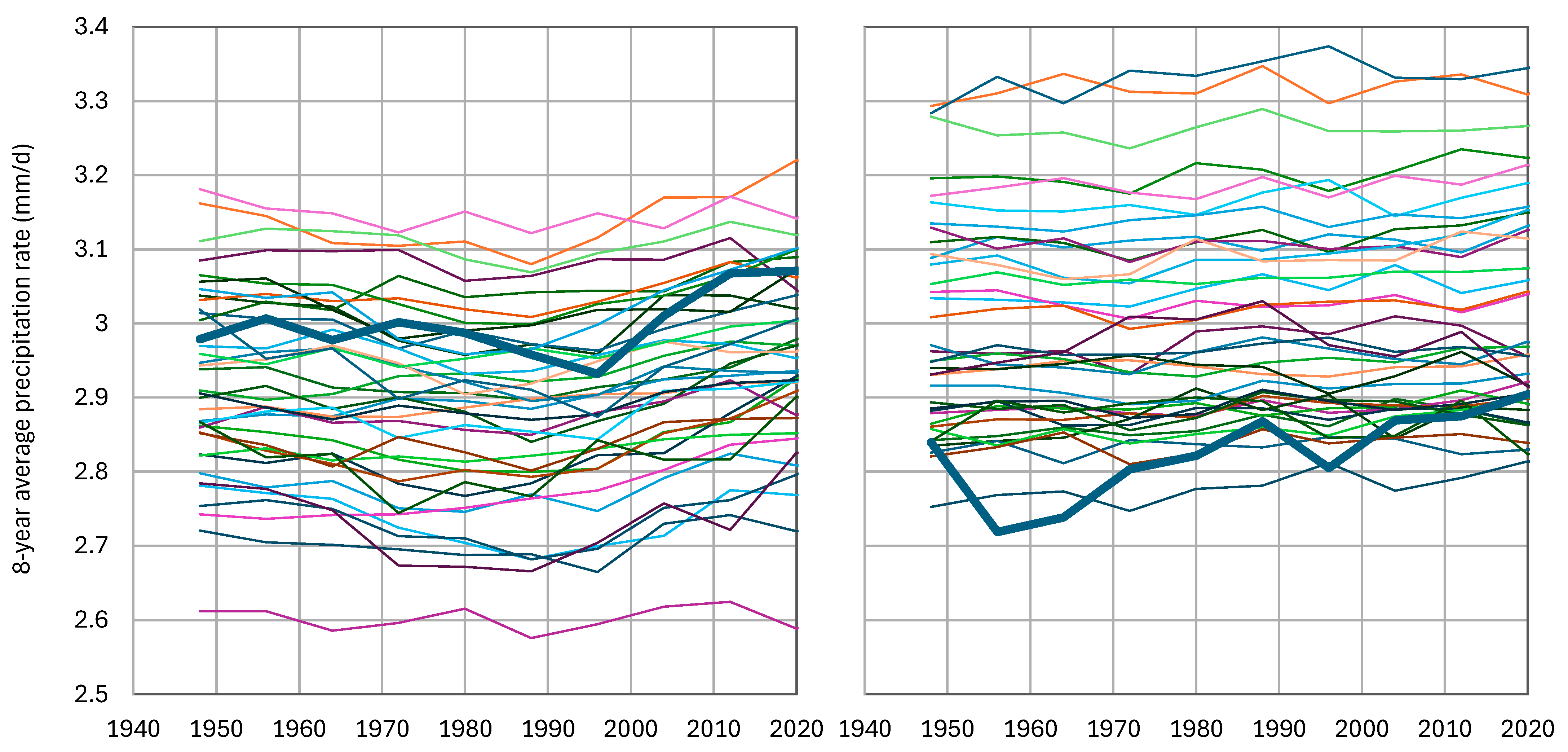
4. Real-World Case Study

To present a large-scale case study of hydrological interest, we use the results of climate models for precipitation, which have been very popular and widely used in so-called climate impact studies, but without proper testing to see whether they are useful or not. The climate models (also known as global circulation models—GCM) that are used belong to the last-generation Coupled Model Intercomparison Project (CMIP6), and their outputs for precipitation were retrieved from the Koninklijk Nederlands Meteorologisch Instituut (KNMI) Climate Explorer [28,29]. The outputs from the 37 models listed in

Table 3. The CMIP6 climate models (GCMs) whose results are used in this study.

#	CMIP6 GCM	#	CMIP6 GCM	#	CMIP6 GCM	#	CMIP6 GCM
1	ACCESS-CM2	11	CIESM	21	GFDL-CM4	31	MPI-ESM1-2-HR
2	ACCESS-ESM1-5	12	CMCC-CM2-SR5	22	GFDL-ESM4	32	MPI-ESM1-2-LR
3	AWI-CM-1-1-MR	13	CNRM-CM6-1 f2	23	GISS-E2-1-G-p3	33	MRI-ESM2-0
4	BCC-CSM2-MR	14	CNRM-CM6-1-HR f2	24	HadGEM3-GC31-LL f3	34	NESM3
5	CAMS-CSM1-0	15	CNRM-ESM2-1-f2	25	INM-CM4-8	35	NorESM2-LM
6	CanESM5 p2	16	EC-Earth3	26	INM-CM5-0	36	NorESM2-MM
7	CanESM5-CanOE p2	17	EC-Earth3-Veg	27	IPSL-CM6A-LR	37	UKESM1-0-LL f2
8	CanESM5-p1	18	FGOALS-f3-L	28	KACE-1-0-G
9	CESM2	19	FGOALS-g3	29	MIROC6
10	CESM2-WACCM	20	FIO-ESM-2-0	30	MIROC-ES2L f2

were available on a monthly scale and were aggregated to annual and over-annual scales.

To make time series that represent reality, the gridded data of the ERA5 reanalysis were used [30,31]. This is the fifth-generation atmospheric reanalysis of the European Centre for Medium-Range Weather Forecasts (ECMWF), where the name ERA refers to ECMWF ReAnalysis. ERA5 has been produced as an operational service, and its fields compare well with the ECMWF operational analyses. It combines vast amounts of historical observations into global estimates using advanced modeling and data assimilation systems. The data are available for the period 1940–now at a spatial resolution of 0.5° globally and were retrieved using the Web-based Reanalyses Intercomparison Tools (WRIT) [32], made available by the USA National Oceanic and Atmospheric Administration (NOAA).

Several studies have evaluated the reliability of ERA5 precipitation data. Koutsoyiannis [33] conducted a global comparison with other datasets, including the Global Precipitation Climatology Project (GPCP) dataset, which integrates gauge and satellite precipitation data over a global grid. His analysis revealed that ERA5 precipitation data closely align with GPCP observations on an annual scale across land, sea, and the entire globe. Similarly, Hassler and Lauer [34] observed good agreement between ERA5 and satellite-based observations in Central Europe and the South Asian Monsoon region, although ERA5 underestimated very low precipitation rates in tropical regions. Bandhauer et al. [35] found that while ERA5 shows qualitative agreement with reference datasets, it overestimates mean precipitation in all regions due to an excessive number of wet days. In contrast, Longo-Minnolo et al. [36] analyzed ERA5-Land precipitation data at the catchment scale in Sicily (Italy) and identified an underestimation, highlighting the need for adjustments to address local microclimatic conditions. The ERA5 precipitation was used as a benchmark by Cavalleri et al. [37] to validate other high-resolution regional reanalyses over Italy. Improvements in the ERA5 precipitation estimates are discussed by Lavers et al. [38].

Comparisons of models and reality, represented by ERA5, were made for the period 1940–2023 (84 years), separately for the North Hemisphere (NH) and the South Hemisphere (SH). A visual comparison of the time series is presented using spaghetti graphs in Figure 5 on the annual scale (annual precipitation rate averaged over a hemisphere) and Figure 6 on an 8-year scale (8-year average of the annual series). The latter was selected as the maximum climatic scale that allows 10 data points, so that statistics can be estimated with some reliability.

A prominent characteristic seen in the spaghetti graphs is the large bias of models, which is mostly negative for the NH and mostly positive for the SH. Different models have largely different biases, which in most of them are very large. The large bias in precipitation certainly reflects the inappropriate modeling of the physical processes related to the hydrological cycle, starting with latent heat and evaporation.

Nonetheless, Figure 7 shows that on a hemispheric basis, there is a correlation between models and reality, with an average of 0.31 for the NH and 0.11 for the SH. An interesting property is that each model’s precipitation at the NH is negatively correlated to that of the same model for the SH, with an average correlation of −0.61 for zero lag. This model property, however, does not correspond to reality: if this correlation is estimated from the ERA5 data, it is practically zero (−0.03). If we take cross-correlations lagged by one year, their values are close to zero for the models in both directions of lagging (one is shown in the rightmost panel of Figure 7) but slightly positive (0.29) for the ERA5 data.

These correlations are not enough to suggest the usefulness of the models in terms of the explained variation. As seen in Figure 8, both classical and K-explained variance are mostly negative on an annual scale. Yet, positive values appear on the 8-year scale. However, if we also consider the bias, which is shown in Figure 9, the total efficiency metrics, NSE and KAEE, take highly negative values, which prevent the climate models from being at all useful for hydrological purposes.

The most relevant question is whether or not some of the models have relatively good performance in general. To study this question, we first assess which of the models have the best performance, in a Pareto optimality sense, for both hemispheres. To this aim, we plot in Figure 10 the cross-performance of the GCMs for both hemispheres in terms of the K-explained variation, KEV₂, on annual and 8-year time scales. On the annual scale, the models show mostly negative explained variation, that is, poor performance. On the 8-year scale, the performance is improved. The two models with the least poor performance appear to be CMCC-CM2-SR5 and FGOALS-f3-L.

The change in the performance with the moment order and time scale for the CMCC-CM2-SR5 model is shown in Figure 11, where it is seen that for small time scales, the performance is not good in either hemisphere. Figure 12 shows that the performance at the annual scale can be slightly improved by applying the transformation of Equation (37), but this is accompanied by a worsening of the performance at large time scales. Interestingly, the improvement at the annual scale is due to the linear part of the transformation, namely on the parameter $\beta =0.41\ne 1$, and not due to the logarithmic part.

The next step is to choose an area smaller than an entire hemisphere and assess the performance of the two “least poor” models in this area. Given that ERA5 is developed in Europe and hence expected to be more accurate in this area, we chose a spherical rectangle that contains Europe, namely that defined by the coordinates 11° W, 40° E, 34° N, and 71° N. The time series of the two models in question, integrated over this area, are shown in Figure 13, in comparison with the ERA5 time series. The visual comparison is not encouraging in terms of the agreement of the models with reality.

Even without considering the bias, which is substantial, i.e., by only considering the explained variation, the results are rather disappointing, with ${\mathrm{KEV}}_2^{\left(\kappa \right)}$ not exceeding 0.1 at any scale $\kappa$ (Figure 14).

5. Discussion and Conclusions

The classical Nash–Sutcliffe efficiency appears to be a good metric of the appropriateness of a model. Yet its fusion of two different characteristics, the explained variance and the bias, is not always useful. The bias could be a very important characteristic to consider for a physically based model, where the bias reflects a violation of a physical law (e.g., conservation of mass or energy). In such cases, a large bias would be a sufficient reason to reject a model, even if it captures the variation patterns.

In other cases, in which the model is of a conceptual or statistical, rather than physical, type, the bias can be easily removed by a shift in the origin. In such cases, a nonlinear transformation of the observed and modeled series, accompanied by a linear transformation of the simulated series (Equations (36) and (37)), can potentially improve the agreement between the model and reality. It is suggested that in such cases, the quantified assessment of model usefulness be based on the metrics of both the original and the transformed series.

The typical metrics that are currently used to assess model performance are based on classical statistics up to a second order. This is not a problem when the processes are Gaussian, but most hydrological processes are non-Gaussian. The concept of knowable moments (K-moments) offers us a basis for extending the performance metrics to high orders, up to the sample size. The two metrics proposed, the K-unexplained variation, ${\mathrm{KUV}}_p$, and the K-bias, ${\mathrm{KB}}_p$, both based on K-moments of the model error, provide ideal means to assess the agreement of models with reality; the closer to zero they are, the better the agreement. The lowest order on which they are evaluated is $p=2$, which represents second-order properties, but also using higher orders gives useful information on the agreement of the entire distribution functions.

The real-world application presented is a large-scale comparison of climatic model outputs for precipitation with reality over the last 84 years. It turns out that the precipitation simulated by the climate models does not agree with reality on the annual scale, but there is some improvement on larger time scales on a hemispheric basis. However, when the areal scale is decreased from hemispheric to continental, i.e., when Europe is examined, the model performance is poor even at large time scales. Therefore, the usefulness of climate model results for hydrological purposes is doubtful.

References

1. Box, G.E.P. Robustness in the Strategy of Scientific Model Building. In Robustness in Statistics; Launer, R.L., Wilkinson, G.N., Eds.; Academic Press: New York, NY, USA, 1979; pp. 201–236. ISBN 978-0-12-438150-6. [Google Scholar] [CrossRef]
2. Koutsoyiannis, D.; Montanari, A. Negligent killing of scientific concepts: The stationarity case. Hydrol. Sci. J. 2015, 60, 1174–1183. [Google Scholar] [CrossRef]
3. Kurshan, R. Computer-Aided Verification of Coordinating Processes: The Automata-Theoretic Approach; Princeton University Press: Princeton, NJ, USA, 1994; ISBN 0-691-03436-2. [Google Scholar]
4. Nash, J.E.; Sutcliffe, J.V. River flow forecasting through conceptual models, part I—A discussion of principles. J. Hydrol. 1970, 10, 282–290. [Google Scholar] [CrossRef]
5. Koutsoyiannis, D.; Kundzewicz, Z.W. Editorial—Quantifying the impact of hydrological studies. Hydrol. Sci. J. 2007, 52, 3–17. [Google Scholar] [CrossRef]
6. Willmott, C.J.; Ackleson, S.G.; Davis, R.E.; Feddema, J.J.; Klink, K.M.; Legates, D.R.; O’Donnell, J.; Rowe, C.M. Statistics for the evaluation and comparison of models. J. Geophys. Res. Ocean. 1985, 90, 8995–9005. [Google Scholar] [CrossRef]
7. Willmott, C.J.; Robeson, S.M.; Matsuura, K. A refined index of model performance. Int. J. Climatol. 2012, 32, 2088–2094. [Google Scholar] [CrossRef]
8. Bennett, N.D.; Croke, B.F.; Guariso, G.; Guillaume, J.H.; Hamilton, S.H.; Jakeman, A.J.; Marsili-Libelli, S.; Newham, L.T.; Norton, J.P.; Perrin, C.; et al. Characterising performance of environmental models. Environ. Model. Softw. 2013, 40, 1–20. [Google Scholar] [CrossRef]
9. Huang, C.; Chen, Y.; Zhang, S.; Wu, J. Detecting, extracting, and monitoring surface water from space using optical sensors: A review. Rev. Geophys. 2018, 56, 333–360. [Google Scholar] [CrossRef]
10. Reichstein, M.; Camps-Valls, G.; Stevens, B.; Jung, M.; Denzler, J.; Carvalhais, N.; Prabhat, F. Deep learning and process understanding for data-driven Earth system science. Nature 2019, 566, 195–204. [Google Scholar] [CrossRef] [PubMed]
11. Zurell, D.; Franklin, J.; König, C.; Bouchet, P.J.; Dormann, C.F.; Elith, J.; Fandos, G.; Feng, X.; Guillera-Arroita, G.; Guisan, A.; et al. A standard protocol for reporting species distribution models. Ecography 2020, 43, 1261–1277. [Google Scholar] [CrossRef]
12. Peng, S.; Ding, Y.; Liu, W.; Li, Z. 1 km monthly temperature and precipitation dataset for China from 1901 to 2017. Earth Syst. Sci. Data 2019, 11, 1931–1946. [Google Scholar] [CrossRef]
13. Hassani, A.; Azapagic, A.; Shokri, N. Predicting long-term dynamics of soil salinity and sodicity on a global scale. Proc. Natl. Acad. Sci. USA 2020, 117, 33017–33027. [Google Scholar] [CrossRef] [PubMed]
14. Hassani, A.; Azapagic, A.; Shokri, N. Global predictions of primary soil salinization under changing climate in the 21st century. Nat. Commun. 2021, 12, 6663. [Google Scholar] [CrossRef] [PubMed]
15. Yaseen, Z.M. An insight into machine learning models era in simulating soil, water bodies and adsorption heavy metals: Review, challenges and solutions. Chemosphere 2021, 277, 130126. [Google Scholar] [CrossRef] [PubMed]
16. Naser, M.Z.; Alavi, A.H. Error metrics and performance fitness indicators for artificial intelligence and machine learning in engineering and sciences. Archit. Struct. Constr. 2023, 3, 499–517. [Google Scholar] [CrossRef]
17. Martinho, A.D.; Hippert, H.S.; Goliatt, L. Short-term streamflow modeling using data-intelligence evolutionary machine learning models. Sci. Rep. 2023, 13, 13824. [Google Scholar] [CrossRef] [PubMed]
18. O’Connell, P.E.; Koutsoyiannis, D.; Lins, H.F.; Markonis, Y.; Montanari, A.; Cohn, T.A. The scientific legacy of Harold Edwin Hurst (1880–1978). Hydrol. Sci. J. 2016, 61, 1571–1590. [Google Scholar] [CrossRef]
19. Hurst, H.E. Long-Term Storage Capacity of Reservoirs. Trans. Am. Soc. Civ. Eng. 1951, 116, 770–799. [Google Scholar] [CrossRef]
20. Gupta, H.V.; Kling, H. On typical range, sensitivity, and normalization of Mean Squared Error and Nash-Sutcliffe Efficiency type metrics. Water Resour. Res. 2011, 47, W10601. [Google Scholar] [CrossRef]
21. Kling, H.; Fuchs, M.; Paulin, M. Runoff conditions in the upper Danube basin under an ensemble of climate change scenarios. J. Hydrol. 2012, 424, 264–277. [Google Scholar] [CrossRef]
22. Lombardo, F.; Volpi, E.; Koutsoyiannis, D.; Papalexiou, S.M. Just two moments! A cautionary note against use of high-order moments in multifractal models in hydrology. Hydrol. Earth Syst. Sci. 2014, 18, 243–255. [Google Scholar] [CrossRef]
23. Koutsoyiannis, D. Knowable moments for high-order stochastic characterization and modelling of hydrological processes. Hydrol. Sci. J. 2019, 64, 19–33. [Google Scholar] [CrossRef]
24. Koutsoyiannis, D. Replacing histogram with smooth empirical probability density function estimated by K-moments. Sci 2022, 4, 50. [Google Scholar] [CrossRef]
25. Koutsoyiannis, D. Knowable moments in stochastics: Knowing their advantages. Axioms 2023, 12, 590. [Google Scholar] [CrossRef]
26. Koutsoyiannis, D. Stochastics of Hydroclimatic Extremes—A Cool Look at Risk, 3rd ed.; Kallipos Open Academic Editions: Athens, Greece, 2023; 391p, ISBN 978-618-85370-0-2. [Google Scholar] [CrossRef]
27. Koutsoyiannis, D.; Yao, H.; Georgakakos, A. Medium-range flow prediction for the Nile: A comparison of stochastic and deterministic methods. Hydrol. Sci. J. 2008, 53, 142–164. [Google Scholar] [CrossRef]
28. Trouet, V.; Van Oldenborgh, G.J. KNMI Climate Explorer: A web-based research tool for high-resolution paleoclimatology. Tree-Ring Res. 2013, 69, 3–13. [Google Scholar] [CrossRef]
29. The KNMI Climate Explorer. Available online: https://climexp.knmi.nl/start.cgi (accessed on 19 August 2024).
30. ERA5: Data Documentation—Copernicus Knowledge Base—ECMWF Confluence Wiki. Available online: https://confluence.ecmwf.int/display/CKB/ERA5%3A+data+documentation (accessed on 25 March 2023).
31. Soci, C.; Hersbach, H.; Simmons, A.; Poli, P.; Bell, B.; Berrisford, P.; Horányi, A.; Muñoz-Sabater, J.; Nicolas, J.; Radu, R.; et al. The ERA5 global reanalysis from 1940 to 2022. Q. J. R. Meteorol. Soc. 2024, 150, 4014–4048. [Google Scholar] [CrossRef]
32. Web-Based Reanalyses Intercomparison Tools. Available online: https://psl.noaa.gov/data/atmoswrit/timeseries/index.html (accessed on 19 August 2024).
33. Koutsoyiannis, D. Revisiting the global hydrological cycle: Is it intensifying? Hydrol. Earth Syst. Sci. 2020, 24, 3899–3932. [Google Scholar] [CrossRef]
34. Hassler, B.; Lauer, A. comparison of reanalysis and observational precipitation datasets including ERA5 and WFDE5. Atmosphere 2021, 12, 1462. [Google Scholar] [CrossRef]
35. Bandhauer, M.; Isotta, F.; Lakatos, M.; Lussana, C.; Båserud, L.; Izsák, B.; Szentes, O.; Tveito, O.E.; Frei, C. Evaluation of daily precipitation analyses in E-OBS (v19. 0e) and ERA5 by comparison to regional high-resolution datasets in European regions. Int. J. Climatol. 2022, 42, 727–747. [Google Scholar] [CrossRef]
36. Longo-Minnolo, G.; Vanella, D.; Consoli, S.; Pappalardo, S.; Ramírez-Cuesta, J.M. Assessing the use of ERA5-Land reanalysis and spatial interpolation methods for retrieving precipitation estimates at basin scale. Atmos. Res. 2022, 271, 106131. [Google Scholar] [CrossRef]
37. Cavalleri, F.; Lussana, C.; Viterbo, F.; Brunetti, M.; Bonanno, R.; Manara, V.; Lacavalla, M.; Sperati, S.; Raffa, M.; Capecchi, V.; et al. Multi-scale assessment of high-resolution reanalysis precipitation fields over Italy. Atmos. Res. 2024, 312, 107734. [Google Scholar] [CrossRef]
38. Lavers, D.A.; Hersbach, H.; Rodwell, M.J.; Simmons, A. An improved estimate of daily precipitation from the ERA5 reanalysis. Atmos. Sci. Lett. 2024, 25, e1200. [Google Scholar] [CrossRef]
Figure 1. Relationship of KGE and NSE for μ s _ = μ x _ and the indicated values of σ s _ / σ x _ . LC stands for the limiting curve corresponding to r s _ x _ = 1 , for which KGE = 1 1 EV . Nb., for r s _ x _ = 1 KGE is 1 (precisely when EV = 3 or somewhat smaller for different EV values).
Water 17 00264 g001
Figure 3. Performance metrics for the original, the logarithmically transformed, and the final λ-transformed series (as seen in Figure 2), namely K-explained variation, KEV p κ , as a function of (left) order p for time scale κ = 1 ; (right) time scale κ for order p = 2 .
Water 17 00264 g003
Figure 4. Model bias metrics for the original, the logarithmically transformed, and the final λ-transformed series (Figure 2), as a function of order p for time scale κ = 1 : (left) ratio R p ; (right) K-bias KB p .
Water 17 00264 g004
Figure 5. Spaghetti graphs of modeled annual average precipitation (thin lines) by the 37 CMIP6 GCMs in comparison to the ERA5 reanalysis data (thick line) for (left) NH and (right) SH.
Water 17 00264 g005
Figure 6. Spaghetti graphs of modeled 8-year average precipitation (thin lines) by the 37 CMIP6 GCMs in comparison to the ERA5 reanalysis data (thick line) for (left) NH and (right) SH.
Water 17 00264 g006
Figure 7. Box plots of the correlation coefficients between annual time series of (left two panels) GCM models and ERA5 reanalysis for NH and SH, respectively, and (right two panels) the same GCM models for NH and SH for lags 0 (concurrent values for NH and SH) and 1 (SH lagged 1 year after NH). Data points are marked with “◦” and their mean value is marked with “✕”.
Water 17 00264 g007
Figure 8. Box plots of (upper) explained variance, EV, and (lower) K-explained variation, KEV2, for the indicated cases (NH/SH; annual/8-year scales).
Water 17 00264 g008
Figure 9. Box plots of (upper) K-bias, KB2, (middle) Nash–Sutcliffe efficiency (NSE), and (lower) K-absolute error efficiency, KAEE, for the indicated cases (NH/SH; annual/8-year scales).
Water 17 00264 g009
Figure 10. Cross-performance at both hemispheres of the GCMs, in terms of K-explained variation, KEV2, at time scales (left) annual and (right) 8-year.
Water 17 00264 g010
Figure 11. Performance metrics of the CMCC-CM2-SR5 model for the NH and SH, namely K-explained variation, KEV p κ , as a function of (left) order p for time scale κ = 1 ; (right) time scale κ for order p = 2 .
Water 17 00264 g011
Figure 12. Performance metrics of the CMCC-CM2-SR5 model for the NH and for the original and transformed series, namely K-explained variation, KEV p κ , as a function of (left) order p for time scale κ = 1 ; (right) time scale κ for order p = 2 .
Water 17 00264 g012
Figure 13. Evolution of the precipitation in the wider area of Europe, defined by the coordinates 11° W 40° E, 34° N, and 71° N at (left) annual and (right) 8-year time scale in comparison to the GCMs with the least poor performance, namely CMCC-CM2-SR5 and FGOALS-f3-L.
Water 17 00264 g013
Figure 14. Performance metrics of the GCMs with the least poor performance, namely CMCC-CM2-SR5 and FGOALS-f3-L for the wider area of Europe, based on the time series seen in Figure 13, namely K-explained variation, KEV p κ , as a function of (left) order p for time scale κ = 1 ; (right) time scale κ for order p = 2 .
Water 17 00264 g014