Diurnal Variation of Carbon Dioxide Concentration and Flux in a River–Lake Continuum of a Mega City

Abstract

The carbon dioxide (CO₂) emissions at the water–air interface in the urban river–lake continuum remain unknown, posing challenges for assessing carbon sinks in aquatic ecosystems draining this unique urban characteristic. This study investigates the driving factors of diurnal variations of CO₂ emission fluxes at the water–air interface in an urban river (Qingshangang, QSG) and a connected landscape lake (Lihu, LH). Continuous monitoring was conducted from 8:00 a.m. to 7:00 p.m. in July 2024 at both QSG and LH sites. The results reveal significant temporal and spatial differences in CO₂ concentration and flux. The CO₂ concentration in QSG (120.91 ± 93.99 μmol L⁻¹) clearly exceeds that of LH (69.14 ± 51.09 μmol L⁻¹), with an overall mean of 95.02 ± 69.69 μmol L⁻¹ for the river–lake system as a whole. The CO₂ flux at QSG (77.53 ± 64.59 mmol m⁻² d⁻¹) is significantly higher than that of LH (53.50 ± 37.32 mmol m ⁻² d ⁻¹), with a total average of 65.51 ± 54.10 mmol m ⁻² d ⁻¹. The concentrations and fluxes were significantly negatively correlated with environmental factors such as pH, dissolved oxygen (DO), percent dissolved oxygen (DO%), water temperature (T_water), chlorophyll (Chl-a), and chemical oxygen demand of manganese (COD_Mn), and significantly positively correlated with electrical conductivity (EC). DO%, EC, and Chl-a are the main environmental factors affecting CO₂ flux by stepwise regression analysis. The considerably higher CO₂ concentration and flux observed in the QSG can be attributed to carbon and nutrient inputs from its surrounding environment. Conversely, the lower CO₂ flux in the connected lake is due to the effective restoration by aquatic plants. Our study underscores the importance of recognizing urban rivers as potential hotspots for CO₂ emissions, thereby emphasizing the imperative for high-time-resolution monitoring efforts on these rivers in future research endeavors.

1. Introduction

Inland waters are an important part of the global carbon cycle, playing an important role in regulating the emission, accumulation, and transport of carbon [1]. Carbon emissions from global inland waters are estimated at 4.40 Pg C per year, comparable to the amount of carbon dioxide (CO₂) absorbed by the oceans [2]. Urban waters, an important part of inland waters, have become hot spots of carbon emission due to their special environmental conditions, such as adequate supply of nutrients, anoxic environment, and temperature conditions suitable for rapid decomposition of organic matter [3]. Urbanization largely increases river CO₂ emissions by increasing nutrient and dissolved organic carbon output to the aquatic environment [4,5]. It is particularly urgent to strengthen the understanding of CO₂ flux in urban rivers due to the eutrophication and the rapid changes in quantity and quality of organic carbon by urbanization.

The quantification of aquatic carbon emissions still faces certain challenges due to uncertainties in observational techniques and model predictions. It is particularly important to continuously monitor the CO₂ concentration in urban water bodies [6]. In addition, there are few comprehensive comparative studies on urban rivers and their connected landscape lakes when studying carbon dioxide emissions in water bodies. As a typical artificial or semi-artificial water body in the urban environment, a landscape lake not only assumes the function of beautifying the surroundings and enhancing urban landscape value, but also plays a certain role in regulating urban microclimate [7]. However, the carbon emission and absorption mechanisms of landscape lakes are often underestimated or even overlooked [8]. The amount of CO₂ emitted in landscape lakes is about the same as in regional-scale lakes, and stream methane emissions are an important part of the regional greenhouse gas balance [9]. It has been found that urban landscape water may play the dual role of carbon source or carbon sink on different time scales, with CO₂ flux being especially significant [10].

In this study, we conducted continuous daytime measurements of CO₂ concentration and flux in an urban river (Qingshangang, QSG) and a connected landscape lake (Lihu, LH), briefly called a river–lake continuum. Our goals are to (1) explore the diurnal variation of CO₂ concentration and CO₂ flux in the river–lake continuum, (2) explore differences in CO₂ concentration and flux between the urban river and the landscape lake, and (3) reveal the key drivers of CO₂ concentration and flux. This study aims to enhance the understanding of carbon emission in the urban water system and provide new insight into urban water management of carbon emission reduction.

2. Materials and Methods

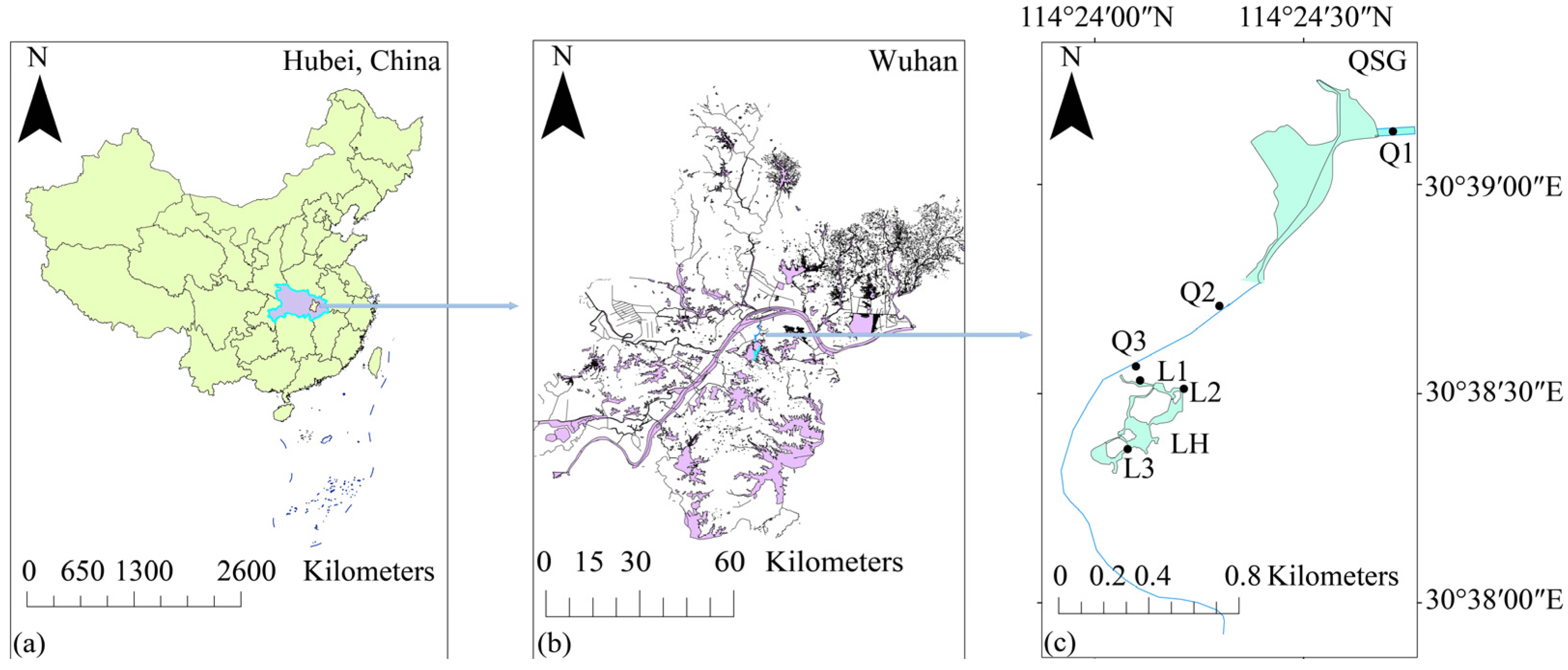
2.1. Study Area

Wuhan (29°58′–31°22′ N and 113°41′–115°05′ E) is in the eastern region of Hubei Province, China. The city has many rivers and lakes, and the water area accounts for one-quarter of the total area of the city, which makes it rich in water resources and has led to its designation as an international wetland city. Wuhan has a subtropical monsoon climate with four distinct seasons, featuring cold winters, hot summers (extreme temperatures above 40 °C), and abundant summer rainfall. Wuhan has an annual average rainfall of 1200 mm. The high rainfall often raises water levels in the Yangtze River and its tributaries during the flood season.

The QSG is located in the west of Qingshan District, Wuhan, China, with a total length of 3.9 km from Wufeng Gate in the north to Donghu Port in the south, and is an important connecting hub between the largest urban Lake Donghu’s ecological water network and the Yangtze River. The water flow in QSG is relatively slow, with weak water circulation. The river depth varies significantly across different sections, and water level fluctuations are influenced by seasonal rainfall and the regional drainage system. As an artificial lake, the LH is connected to the QSG and is located inside Qingshan Park, it has the characteristics of a landscape lake, with an area of 30,800 square meters. Due to industrialization and urbanization, the QSG has confronted several issues such as deteriorating water quality. In 2009, the QSG was enlisted as the first batch of pilot projects for the construction of the city’s “sponge city”, and the water quality of the QSG has witnessed significant improvement through the implementation of wetland restoration and sewage treatment. Currently, residential buildings, shopping malls, schools, parks, etc., surround the QSG. These exert a significant impact on biogeochemical processes in the water systems.

In order to investigate the diurnal variation of CO₂ concentration and flux in the QSG, six discrete sample points were chosen (Figure 1). The six sampling sites (Q1–3, L1–3) were sampled in July 2024. Each site was measured consecutively for eleven hours during the day. These sampling sites are as close to the center of the water body as possible. During each sampling period, on-site measurements and water sample collection were carried out every two hours, and a total of 36 water samples were collected during the six campaigns. L1–3 was crystal clear and contained a variety of vegetation for ecological restoration (Hydrilla verticillate (L.f.) Royle; Myriophyllum verticillatum L. and Vallisneria natans (Lour.) H. Hara).

2.2. Sampling and Analyses

Water quality parameters such as pH, water temperature (T_water), dissolved oxygen (DO), percent dissolved oxygen (DO%), and electrical conductivity (EC) were determined on-site by the calibrated CyberScan PCD 650 multi-parameter Water Quality Analyzer (Thermo Fisher Eutech, USA). Wind speed (Uz) and air temperature (T_air) were simultaneously measured by Testo 410-1 portable impeller anemometer (Testo SE & Co. KGaA, Titisee-Neustadt, Germany). Secchi disk depth (SDD) was measured by a Secchi disk. Water samples were collected at 0.2 m below the surface, and were filtered with 0.45 μm and 0.22 μm glass fiber filters on the sampling day. To avoid any headspace or air bubbles, the collected water samples in the 2.5 L high-density polyethylene (HDPE) containers should be filled and sealed.

2.3. Water Chemical Parameters Measurements

The pre-treated water samples were stored in a refrigerator at 4 °C, and all measurements were completed within one week of field sampling. DOC concentration was determined by Total Organic Carbon (TOC) analyzer (TOC-L, Shimadzu, Kyoto, Japan). Chemical oxygen demand in the permanganate index (COD_Mn) was determined by the potassium permanganate index method. All chemical parameters such as total dissolved nitrogen (TDN), nitrate nitrogen (NO₃⁻-N), nitrite nitrogen (NO₂⁻-N), ammonia nitrogen (NH₄⁺-N), total dissolved phosphorus (TDP), phosphate (PO₄³⁻-P), and Chlorophyll-a (Chl-a) were determined in accordance with Chinese National Standard Method [11].

2.4. Continuous CO₂ Measurements

The non-dispersive infrared CO₂ meter (Mini CO₂, Pro-Oceanus, Canada) was employed to continuously monitor the CO₂ concentration in situ. The sensor diffuses the dissolved gas in the freshwater to the infrared detector via a semi-permeable membrane and periodically eliminates CO₂ and records a new baseline value through an automatic zero compensation function, guaranteeing long-term signal stability and continuous measurement. The sensor is placed in the river–lake continuum before 8:00 to achieve environmental balance based on the manual. The data of CO₂ concentration are recorded in ppm with an interval of 5 s, which is converted to μmol L⁻¹ for calculation. Additionally, 100 mL air samples were collected daily in the morning, noon, and afternoon at 1 m above the water surface and measured using a flame-ionized gas chromatograph (GC-2014, Shimadzu, Japan).

2.5. CO₂ Flux Estimations

The CO₂ fluxes F (mmol m⁻² d⁻¹) at the water–air interface are computed by employing the thin-boundary layer (TBL) model [12] as follows:

F = 0.24 × k × H^cp (C_water − C_air),

(1)

where F represents the CO₂ flux at the water–gas interface (mmol m⁻² d⁻¹), 0.24 is the unit conversion coefficient (cm H⁻¹ to m d⁻¹), and C_water refers to the concentration of dissolved CO₂ in waters (ppm). C_air indicates the concentration of CO₂ in the ambient air at each sampling point (ppm), and H^cp represents the solubility constant of Henry’s Law (mol L⁻¹ atm⁻¹).

lnH^cp = −58.0931 + 90.5069 × (100/T_water) + 22.2940 × ln(100/T_water),

(2)

k = k600 × (Sc/600)⁻ⁿ,

(3)

k600 = 2.07 + 0.215 × U₁₀^1.7 (U₁₀ < 3 m s⁻¹),

(4)

k600 = 0.45 × U₁₀^1.64 (3 < U₁₀ < 5 m s⁻¹),

(5)

Sc = 1911.1 − 118.11 × Tw + 3.4527 × T_water² − 0.04132 × T_water³,

(6)

U₁₀ = 1.22 × U_Z.

(7)

Henry’s law, a solubility constant, depends on the water temperature, and the gas transfer coefficient k depends on the wind speed [13]. k600 is the gas transfer velocity with a Schmidt constant equal to 600 at 20 °C and Sc is the Schmidt constant at t °C. When the wind speed measured at a height of one meter is less than 3 m s⁻¹, the Schmidt index n is 0.67, while when the wind speed is greater than 3 m s⁻¹, the Schmidt index n is 0.5 [14]. U₁₀ is the wind speed of 10 m, which is converted from the wind speed of 1 m. U_Z is the wind speed measured every two hours in the field. The wind speed measured represents the average wind speed during the adjacent two-hour period; for example, the wind speed measured at 10:00 is used for the speed during the two hours between 9:00 and 11:00.

2.6. Statistical Analysis

First and foremost, we examined the data normality and discovered that the majority of the indices were not normally distributed. Secondly, a single-factor analysis of variance (ANOVA) test was implemented to analyze the spatio-temporal parameters. Spearman’s non-parametric correlation analysis was employed to disclose the relationships between aquatic CO₂ concentration, flux, and environmental factors. Principal component analysis (PCA) was utilized to analyze the relationship between CO₂ concentration and flux and water environment parameters. In addition, stepwise regression analysis was also used to identify the main factors influencing CO₂ concentration and flux with CO₂ concentration and flux as the dependent variable. SPSS 27.0, Origin 2021, and Arcgis 10.8 software were utilized to accomplish all statistical analysis and mapping.

3. Results

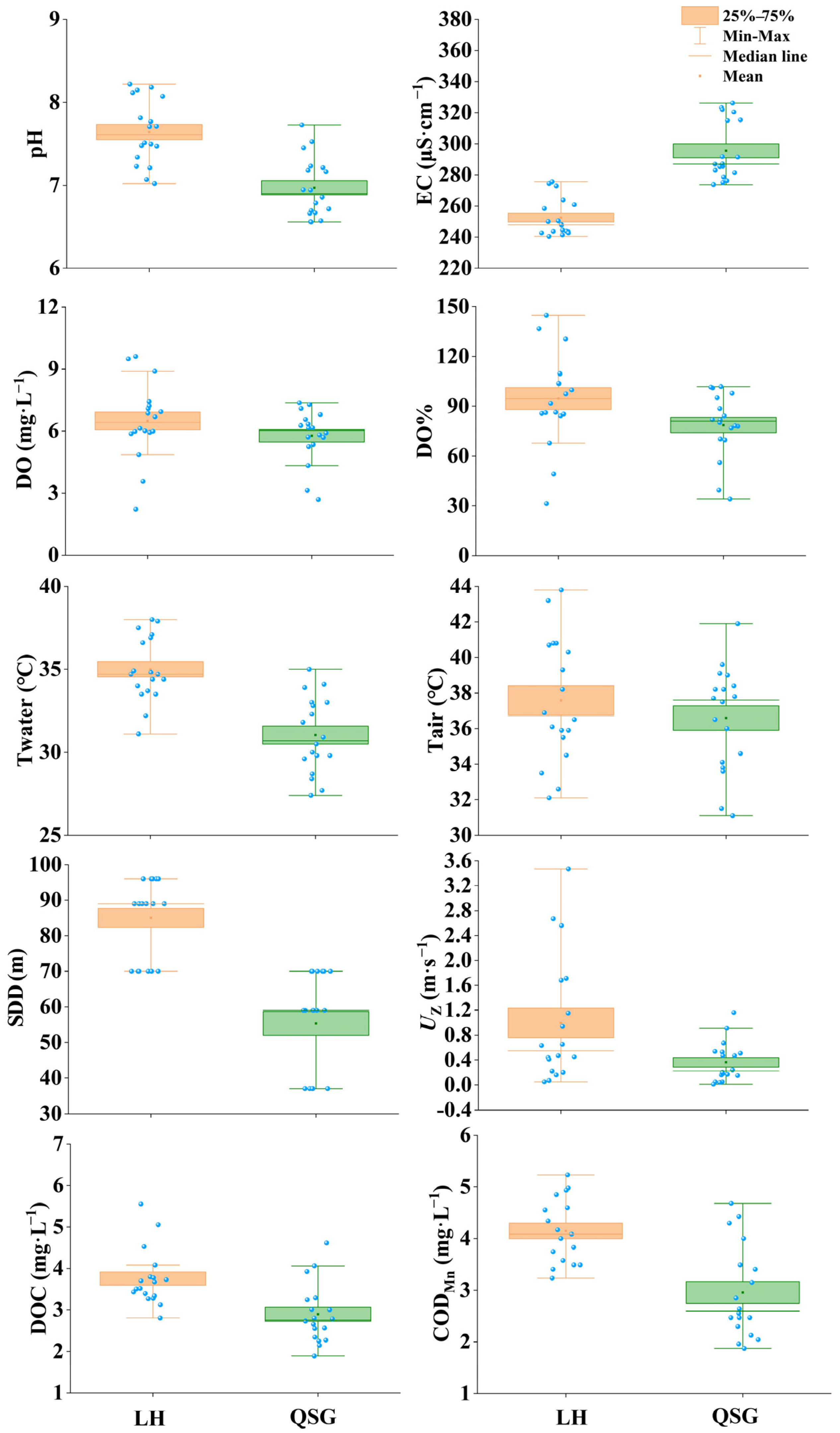
3.1. Physical and Chemical Parameters

The physicochemical parameters in the river–lake continuum showed a similar trend with time (Figures S1 and S2). The pH, DO, and DO% demonstrate an upward trend, while EC shows a downward trend. The T_water and T_air present an upward trend followed by a downward trend, while SDD remains relatively unchanged. Overall, the levels of pH, T_water, SDD, U_Z, DOC, and COD_Mn are significantly higher in lake LH than those in the river QSG (p < 0.05, Figure 2). However, the concentrations of EC, NO₃⁻-N, NO₂⁻-N, TDP, TDN, and PO₄^3--P are markedly lower in the lake than in the river (p < 0.05, Figure 2 and Figure 3). The Chl-a and NH₄⁺-N concentrations do not show significant differences between the QSG and LH (p > 0.05, Figure 3).

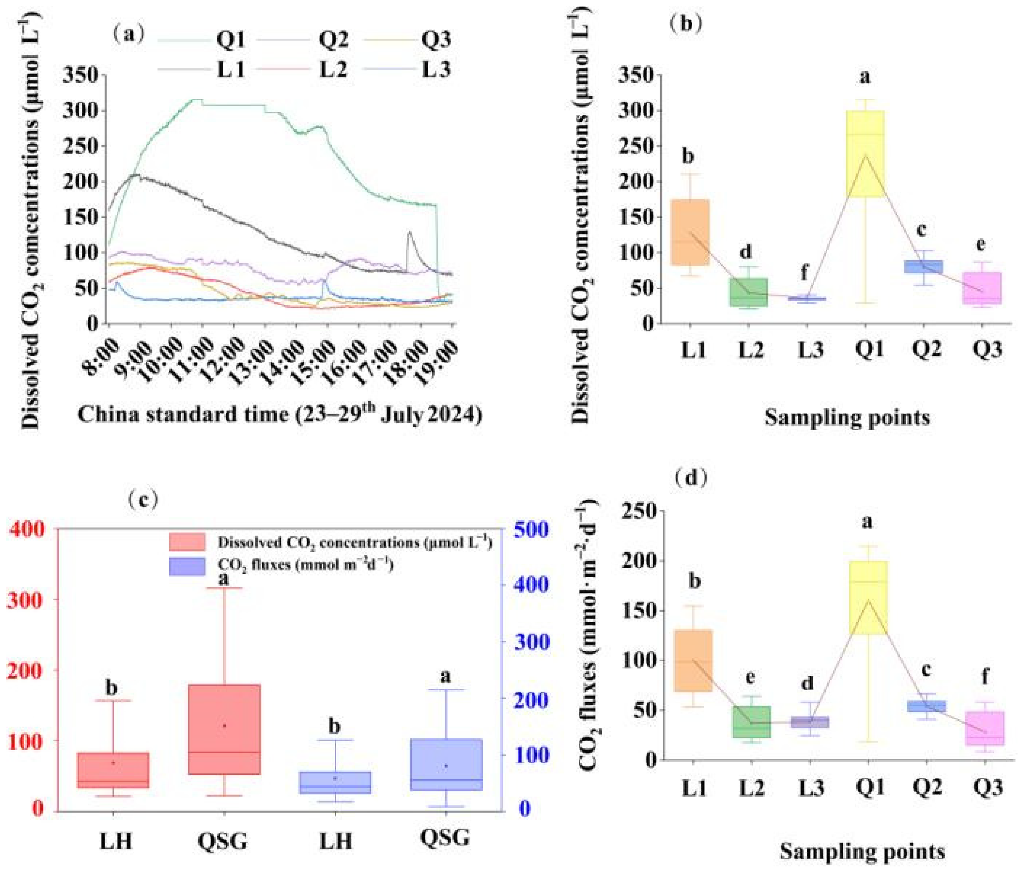
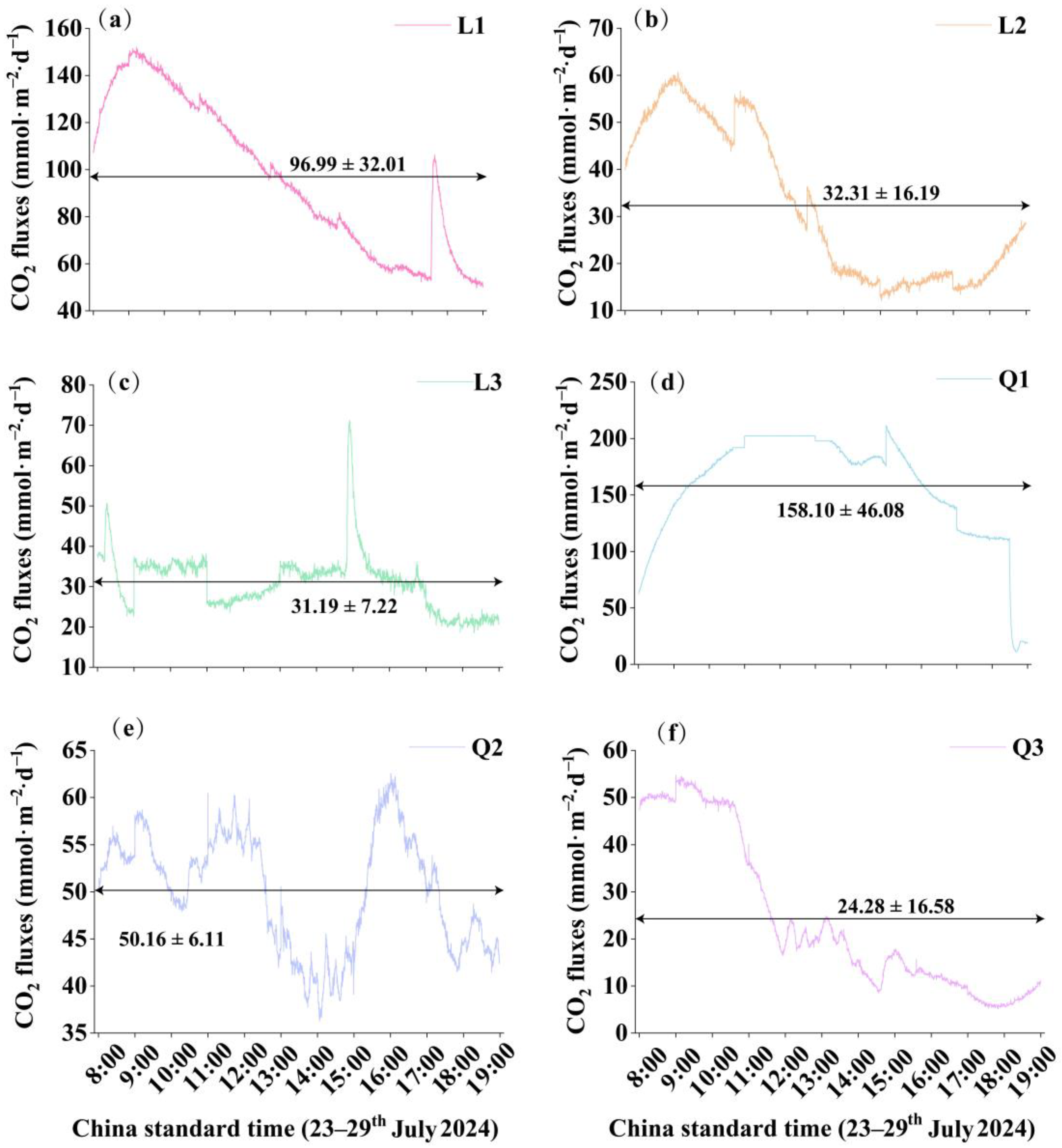
3.2. Diurnal Variation in CO₂ Concentrations and Fluxes

The real-time continuous records of CO₂ concentration and flux over a 6-day period showed that the daily CO₂ concentrations are highly variable (Figure 4). The CO₂ concentration in the site Q1 fluctuated between 29.52 and 316.02 μmol L⁻¹ (Figure 4a). The CO₂ concentration in the Q2 ranged from 54.21 to 102.78 μmol L⁻¹, and CO₂ concentration in the Q3 varied between 22.43 and 86.88 μmol L⁻¹. The concentrations of CO₂ were within the range of 67.28–210.49 μmol L⁻¹ for L1, 21.16–80.20 μmol L⁻¹ for L2, and 29.01–60.92 μmol L⁻¹ for L3 in the three sites of the lake, respectively (Figure 4a). It is notable that the CO₂ concentrations of Q1, Q3, L1, and L2 all peaked during the period between 8:00 and 10:00, with the maximum values of reaching 316.02 μmol L⁻¹ at 10:43 (Q1) and 86.88 μmol L⁻¹ at 8:37 (Q3). The L1 site achieved its maximum value at 9:13 (210.49 μmol L⁻¹), and the L2 site reached its maximum at 9:26 (80.20 μmol L⁻¹). In contrast, the Q2 and L3 reached their maximum in the afternoon, i.e., 16:01 (102.78 μmol L⁻¹, Q2) and 14:54 (60.92 μmol L⁻¹, L3). The lowest concentrations were generally witnessed between 14:00 and 19:00. The lowest values of each point were recorded as follows: 29.52 μmol L⁻¹ at 18:40 in Q1, 54.21 μmol L⁻¹ at 14:04 in Q2, 22.43 μmol L⁻¹ at 17:50 in Q3, 67.28 μmol L⁻¹ at 18:49 in L1, 21.16 μmol L⁻¹ at 15:02 in L2, and 29.01 μmol L⁻¹ at 18:19 in L3 (Figure 4a).

There were significant differences in CO₂ concentration among the six sites (p < 0.01) (Figure 4b), with the highest CO₂ concentration (237.46 ± 69.85 μmol L⁻¹) in Q1 and the lowest (35.86 ± 4.98 μmol L⁻¹) in L3 (Figure 4b). On the whole, the average CO₂ concentration was significantly higher in the QSG (120.91 ± 93.99 μmol L⁻¹) than in the LH (69.14 ± 51.09 μmol L⁻¹) (p < 0.01). The total average value was 95.02 ± 69.69 μmol L⁻¹ in the river–lake systems.

The areal CO₂ fluxes exhibited the characteristic of being a “source”, with an average of 65.51 ± 54.10 mmol m⁻² d⁻¹. The daily CO₂ flux was highly variable, for instance, ranging from 11.17 to 211.57 mmol m⁻² d⁻¹ in Q1, between 36.29 and 62.55 mmol m⁻² d⁻¹ in Q2, and varying from 5.10 to 54.74 mmol m⁻² d⁻¹ in Q3. The CO₂ flux fluctuated between 49.67 and 152.00 mmol m⁻² d⁻¹ in L1, 12.05 and 60.63 mmol m⁻² d⁻¹ in L2, and 18.57–71.16 mmol m⁻² d⁻¹ in L3 (Figure 5). The sites Q1, Q3, L1, and L2 shared the same overall trend, showing a pattern of first increasing and then decreasing. The peaks of the CO₂ fluxes were concentrated in the two time periods of 9:00–10:00 and 14:30–16:30. Among them, the site Q1 reached the maximum value at 15:00 (211.57 mmol m⁻² d⁻¹), the Q2 reached the maximum value at 16:01 (62.55 mmol m⁻² d⁻¹), and the Q3 reached the maximum value at 9:08 (54.74 mmol m⁻² d⁻¹). The L1, L2, and L3 reached their maximum levels at 19:13 (152.00 mmol m⁻² d⁻¹), 9:26 (60.63 mmol m⁻² d⁻¹), and 14:54 (71.16 mmol m⁻² d⁻¹), respectively (Figure 5). The minimum CO₂ fluxes were concentrated in the time period from 17:00 to 19:00 (except for Q2). The Q1 and Q3, respectively, reached their minimum values at 18:40 (11.17 mmol m⁻² d⁻¹) and 17:50 (5.10 mmol m⁻² d⁻¹). The L1, L2, and L3 reached their minimum values at 18:49 (49.67 mmol m⁻² d⁻¹), 17:12 (12.05 mmol m⁻² d⁻¹), and 18:19 (18.57 mmol m⁻² d⁻¹), respectively. The Q2, however, reached its minimum value at 14:04 (36.29 mmol m⁻² d⁻¹) (Figure 5).

There were significant differences in the CO₂ flux among the six sites (p < 0.01, Figure 4d). The Q1 had the largest CO₂ flux (158.10 ± 46.08 mmol m⁻² d⁻¹), and Q3 had the smallest CO₂ flux (24.28 ± 16.58 mmol m⁻² d⁻¹). On the whole, the average CO₂ flux was much higher in the QSG (77.53 ± 64.59 mmol m⁻² d⁻¹) than in the LH (53.50 ± 37.32 mmol m⁻² d⁻¹) (p < 0.01, Figure 4c).

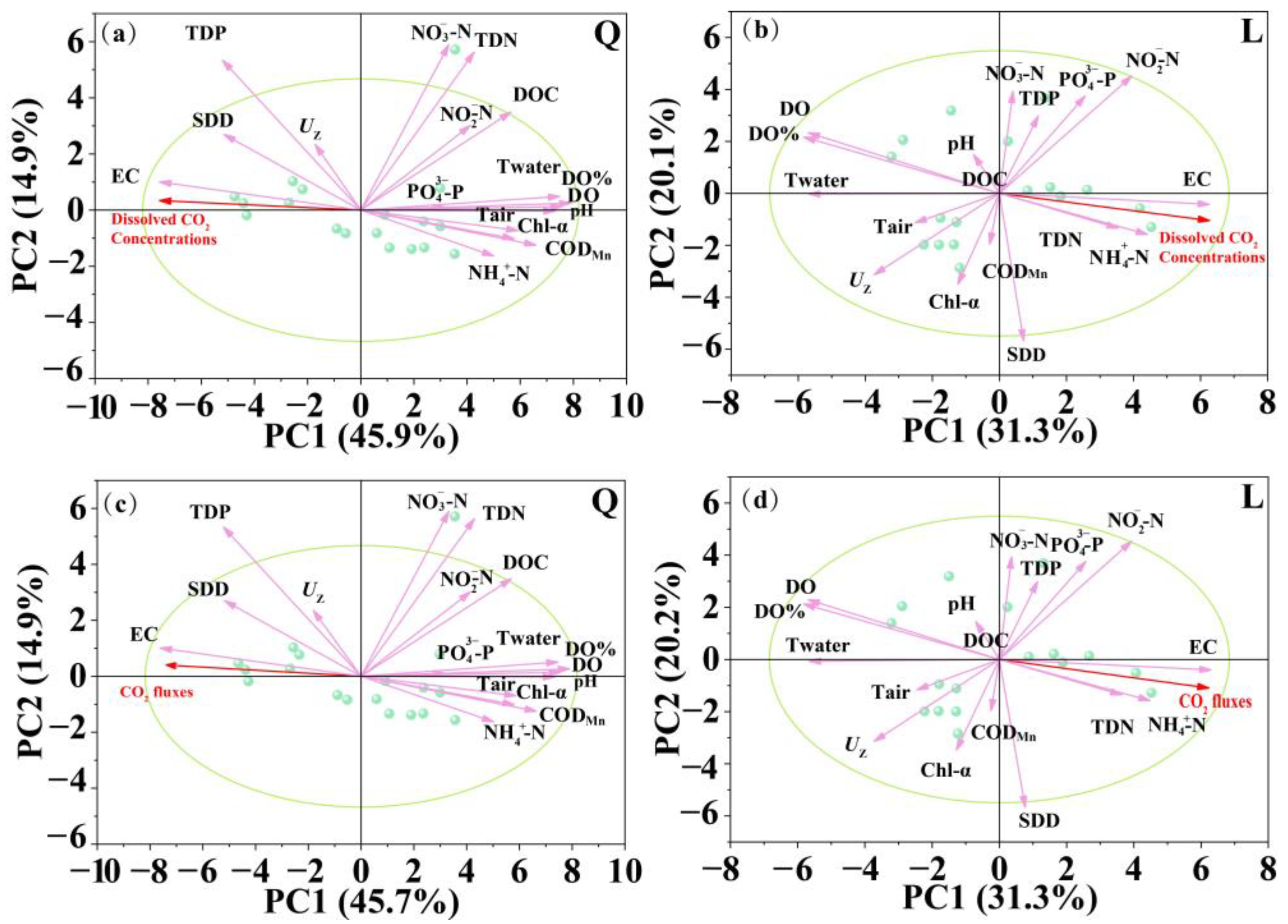
3.3. Relationships Between CO₂ Concentrations and Fluxes with Environmental Variables

On the whole, the CO₂ concentration exhibited significant negative correlations with pH (R² = 0.526, p < 0.01), DO (R² = 0.858, p < 0.01), DO% (R² = 0.909, p < 0.01), T_water (R² = 0.730, p < 0.01), T_air (R² = 0.380, p = 0.022), COD_Mn (R² = 0.563, p < 0.01), Chl-a (R² = 0.558, p < 0.01), and DOC (R² = 0.344, p = 0.040) (

Table 1. Spearman’s correlation coefficients between CO₂ concentration and flux parameters and water parameters.

Parameter	CO2 Concentration	CO2 Flux
pH	−0.526 **	−0.418 *
EC	0.674 **	0.558 **
DO	−0.858 **	−0.853 **
DO%	−0.909 **	−0.857 **
Twater	−0.730 **	−0.590 **
Tair	−0.380	−0.272
UZ	−0.310	−0.212
CODMn	−0.563 **	−0.514 **
DOC	−0.344	−0.316
Chl-a	−0.558 **	−0.570 **
TDN	0.220	−0.054
NO3−-N	0.242	−0.083
NO2−-N	0.226	−0.063
NH4+-N	−0.027	−0.068
TDP	0.429 *	0.267

Notes: * p < 0.05, ** p < 0.01.

), and displayed a positive correlation with EC (R² = 0.674, p < 0.01) and TDP (R² = 0.429, p = 0.016). The CO₂ fluxes were significantly related to pH (R² = 0.418, p = 0.011), DO (R² = 0.853, p < 0.01), DO% (R² = 0.857, p < 0.01), T_water (R² = 0.590, p < 0.01), COD_Mn (R² = 0.514, p < 0.01), and Chl-a (R² = 0.570, p < 0.01), while positively related to EC (R² = 0.558, p < 0.01) (Table 1). The regression models for CO₂ concentration and flux are as follows: cCO₂ (CO₂ concentration) = −129.106 − 1.138DO% + 1.224EC − 1.995Chl-a (p < 0.01, R² = 0.683), FCO₂ = −50.684 − 0.786DO% + 0.720EC − 1.558Chl-a (p < 0.01, R² = 0.625).

To further, respectively, analyze the relationships between CO₂ concentration and flux with environmental variables in the river and lake, data were distinguished (

Table 2. Spearman’s correlation coefficients between CO₂ concentration, flux parameters, and water parameters in landscape lakes and rivers (L: LH, Q: QSG).

Parameter	CO2 Concentration		CO2 Flux
State	L	Q	L	Q
pH	−0.057	−0.789 **	−0.078	−0.740 **
EC	0.774 **	0.845 **	0.821 **	0.853 **
DO	−0.831 **	−0.849 **	−0.844 **	−0.866 **
DO%	−0.862 **	−0.907 **	−0.854 **	−0.909 **
Twater	−0.835 **	−0.728 **	−0.756 **	−0.660 *
Tair	−0.329	−0.312	−0.172	−0.211
UZ	−0.591 **	0.249	−0.492 *	0.238
CODMn	−0.179	−0.886 **	−0.164	−0. 882 **
DOC	0.210	−0.626 **	0.036	−0.624 **
Chl-a	0.039	−0.893 **	−0.019	−0.878 **
TDN	0.376	−0.593 **	0.305	−0.591 *
NO3−-N	0.191	−0.329	0.139	−0.366
NO2−-N	0.527	−0.659 **	0.429	−0.631 **
NH4+-N	0.472 *	−0.434	0.385	−0.432

Notes: * p < 0.05, ** p < 0.01.

). In the QSG, the CO₂ concentration was negatively related to and pH (R² = 0.789, p < 0.01), DO (R² = 0.849, p < 0.01), DO% (R² = 0.907, p < 0.01), T_water (R² = 0.728, p < 0.01), COD_Mn (R² = 0.886, p < 0.01), DOC (R² = 0.626, p < 0.01), Chl-a (R² = 0.893, p < 0.01), TDN (R² = 0.593, p < 0.01), and NO₂⁻-N (R² = 0.659, p < 0.01), while positively related to EC (R² = 0.845, p < 0.01) and TDP (R² = 0.506, p < 0.05) (Table 2). The CO₂ flux was negatively correlated with pH (R² = 0.740, p < 0.01), DO (R² = 0.866, p < 0.01), DO% (R² = 0.909, p < 0.01), T_water (R² = 0.660, p < 0.01), COD_Mn (R² = 0.882, p < 0.01), DOC (R² = 0.624, p < 0.01), Chl-a (R² = 0.878, p < 0.01), TDN (R² = 0.591, p < 0.01), and NO₂⁻-N (R² = 0.631, p < 0.01), but was only positively related to EC (R² = 0.853, p < 0.01) (Table 2). The regression models for CO₂ concentration and flux in the QSG are as follows: cCO₂ = −288.487 + 2.753EC − 1.995T_water (p < 0.01, R² = 0.895), FCO₂ = −640.211 + 2.973EC − 13.762COD_Mn (p < 0.01, R² = 0.625).

Regarding the LH, the CO₂ concentrations were significantly negatively correlated with DO (R² = 0.831, p < 0.01), DO% (R² = 0.862, p < 0.01), T_water (R² = 0.835, p < 0.01), and U_Z (R² = 0.591, p < 0.01), but positively related to EC (R² = 0.774, p < 0.01), NO₂⁻-N (R² = 0.527, p < 0.05), and NH₄⁺-N (R² = 0.472, p < 0.05) (Table 2). The CO₂ flux was significantly negatively correlated with DO (R² = 0.844, p < 0.01), DO% (R² = 0.854, p < 0.01), T_water (R² = 0.756, p < 0.01), and U_Z (R² = 0.492, p < 0.05), but positively correlated with EC (R² = 0.821, p < 0.01) (Table 2). Based on stepwise regression analysis, the models of CO₂ concentration and flux in the LH are as follows: cCO₂ = −1088.621 + 4.083EC (p < 0.01, R² = 0.710), FCO₂ = −755.205 + 2.810EC (p < 0.01, R² = 0.625).

4. Discussion

4.1. Diurnal Variation of CO₂ Concentrations and Fluxes

The results demonstrated the net emission sources of CO₂ (QSG: 77.53 ± 64.59 mmol m⁻² d⁻¹; LH: 53.50 ± 37.32 mmol m⁻² d⁻¹) to the atmosphere from the river–lake continuum (Figure 4c). Urbanization has been shown to greatly alter the biogeochemical processes of rivers and lakes, driving increased CO₂ flux [15,16]. However, the average flux observed in the QSG was clearly lower than the global mean for riverine systems (680 mmol m⁻² d⁻¹) [17]. The CO₂ flux in the QSG was also substantially smaller than that reported for the Chaohu River Basin, another urban river system (900 mmol m⁻² d⁻¹) [4]. This appears to be attributed to ecological restoration efforts. Wang et al. have identified the restoration as an effective strategy for reducing CO₂ emissions in a study on nine urban rivers [18]. Nevertheless, CO₂ fluxes from the LH exceeded the lake fluxes in the same region reported by Zhang et al. [19].

Our results unveiled a trend where CO₂ concentrations initially rise and then subsequently fall, aligning with the observations documented by Yang et al. [20]. This pattern was attributed to the dynamic interplay between photosynthesis and respiration intensity in aquatic environments. During periods of sufficient light, photosynthesis was highly active, effectively consuming atmospheric CO₂ and driving a diurnal decline in CO₂ concentration and flux [21,22]. The CO₂ emissions at sampling points L1 and L3 suddenly increased at 6:00 PM and 3:00 PM, respectively, and can be explained as follows. During the day, aquatic plants (such as algae) absorb CO₂ through photosynthesis, thereby reducing the CO₂ concentration in the water [23]. However, around 3:00 PM, as solar radiation intensity decreases, photosynthesis may gradually weaken, while respiration in aquatic organisms continues, releasing CO₂ into the water. By 6:00 PM, as the sun sets, photosynthesis ceases while respiration persists, further contributing to the rise in CO₂ concentrations [24]. Therefore, during this period, the CO₂ flux in the water increases [25]. Temperature is an important factor affecting the metabolic activities of aquatic organisms. In the afternoon, as solar radiation increases, water temperature may rise, thereby accelerating the respiration of aquatic organisms and increasing CO₂ release [26]. Additionally, human activities may also play a role. Sampling points L1 and L3 are located near areas with significant human activity, such as recreational use or boating, which tend to peak in the afternoon. Human disturbances can stir up sediments or introduce external organic matter (e.g., from runoff or waste), which largely contributes to additional CO₂ [27]. By analyzing the mean values, we determined that the optimal sampling window to represent the average CO₂ flux in lakes was between 12:00 and 14:00, while for rivers, the flux was best captured from 9:00 to 12:00 (Figure 5). These findings had significant ecological implications for understanding carbon dynamics in aquatic systems. The diurnal variations in CO₂ flux highlighted the critical role of photosynthesis in regulating carbon exchange between water and the atmosphere, particularly during daylight hours. Identifying representative sampling periods ensured more accurate assessments of CO₂ emissions and supported the development of reliable carbon budgets. It is worth noting that similar variations in CO₂ fluxes have been observed in subtropical karst reservoirs, where the biological carbon pump effect plays a significant role in carbon sequestration and decreased CO₂ emissions, as reported by Zhang et al. [28], providing further insights into the complex carbon dynamics in different aquatic environments.

4.2. Influencing Factors of CO₂ Concentration and Flux

The key environmental factors affecting the concentration and flux of CO₂ generally include temperature, pH, organic matter, nutrients, etc. [29]. In our study, the environmental factors affecting the concentration and flux of CO₂ include pH, DO, T_water, EC, and Chl-a. The negative correlation observed between CO₂ and pH can be explained as follows. Carbonic acid (H₂CO₃) can easily dissociate into H⁺ and HCO₃⁻ ions in alkaline environments [30], thereby reducing the amount of free CO₂ [31]. At the same time, DO was negatively correlated with CO₂, which was mainly attributed to photosynthesis and respiration. Aquatic plants absorb CO₂ and release O₂ through photosynthesis, resulting in a decrease in CO₂ and an increase in DO content. On the contrary, the respiration of aquatic organisms absorbs O₂ and releases CO₂, resulting in a decrease in O₂ concentration and an increase in CO₂ content [32]. The mechanism of influence of water temperature on CO₂ is complicated. On the one hand, the high-temperature environment promotes microbial activity, accelerates the decomposition of organic carbon, increases the release of CO₂, and may also increase the diffusion rate of CO₂ [33]. For example, the water temperature of an urbanized lake in southwest China has risen significantly with increasing CO₂, which can be explained by this theory [34]. However, in this study, there was a significant negative correlation between water temperature and CO₂, which may be due to the decrease in CO₂ solubility in water indirectly caused by the increase in air temperature, resulting in the decrease in CO₂ in water. A strong negative correlation between CO₂ and water temperature was found in the study of subtropical lakes, which is consistent with the results of this study [35]. As a total index of dissolved ions in water, EC can represent the pollution scale of water [36] and is positively correlated with CO₂. This is consistent with Almeida’s measurements of CO₂ fluxes at the air–water interface in lakes using flow injection analysis [37]. Chl-a represents the primary productivity of water bodies [38] and plays an important role in carbon exchange [39]. CO₂ was significantly negatively correlated with Chl-a (Table 1). Pacheco et al.’s study also found that CO₂ was negatively correlated with Chl-a [40]. These findings illustrate multiple mechanisms by which environmental factors regulate CO₂ dynamics in aquatic systems. By combining these results with existing studies, this paper highlights the environmental dependence of CO₂ flux, emphasizing the role of biological and abiotic factors.

4.3. CO₂ Difference Between Landscape Lake and River

Differences in CO₂ across water bodies are strongly influenced by environmental factors [41,42]. The principal component analysis identified EC, DO, and T_water as key drivers (Figure 6). CO₂ concentrations and fluxes were markedly higher in QSG compared to LH (Figure 2). In the study by Li et al. [43], the CO₂ concentration and flux in the reservoir (artificial lake) are significantly higher than that in the natural lake. The mean CO₂ flux (101.81 ± 186.63 mmol m⁻² d⁻¹) in natural lakes previously reported is about twice that of LH (53.50 ± 37.32 mmol m⁻² d⁻¹). This may be due to the large-scale planting of ecological restoration aquatic grasses in LH. The growth of these aquatic plants can enhance primary productivity and absorb nutrients and suspended solid particles in the water, thus helping to reduce carbon dioxide emissions [44]. We found that the key influencing factors of EC (QGS was higher than LH) and T_water (QSG was lower than LH) contribute to the higher flux of QSG than LH (p < 0.05, Figure 2). Previous studies also reported that CO₂ fluxes are approximately 2–27 times higher in rivers than in lakes in a river–lake system [45]. The mineralization of organic carbon, particularly from allochthonous inputs, directly increases CO₂ concentrations in the water through biological processes [35]. It has been shown that soil-derived organic matter mineralization can sustain more than half of the CO₂ emitted from river networks, so the CO₂ concentration in the river may depend more on organic degradation [46]. Approximately 35% of the organic matter in river-suspended solids underwent extensive degradation, significantly contributing to carbon dioxide emissions [47]. The slow flow velocity of QSG, resembling that of stillwater, provides favorable conditions for the accumulation and bioutilization of organic matter, leading to elevated CO₂ emissions. Furthermore, the higher nutrient content in rivers compared to lakes promotes organic matter decomposition, exacerbating CO₂ release [45,48], as refleced by the much higher levels of TDN, NO₃⁻-N, NO₂⁻-N, TDP, and PO₄³⁻-P in the QSG than the LH (p < 0.05, Figure 3). The establishment of aquatic vegetation, in addition to improving water quality, enhances the carbon sink capacity of lakes [49]. The lower CO₂ emissions observed in LH are likely attributable to the extensive coverage of ecological restoration of aquatic grasses.

These findings underscore the critical role of ecological restoration in regulating carbon dynamics in urban aquatic systems. The establishment of aquatic vegetation not only reduces CO₂ emissions but also supports carbon sequestration, contributing to climate mitigation efforts. Additionally, understanding the mechanisms driving differences in CO₂ fluxes between rivers and lakes is essential for managing freshwater ecosystems under increasing anthropogenic pressures.

5. Conclusions

In this study, CO₂ concentrations in the river–lake continuum QSG and LH are measured in real time and continuously, revealing the dynamic characteristics of CO₂ concentration and flux in urban aquatic systems. The results demonstrate that both the QSG and LH act as net sources of CO₂, with pronounced daily fluctuations in concentration and flux. CO₂ concentrations and fluxes are higher in the river compared to the connected lake, with key influencing factors including pH, DO, T_water, and EC. The characteristics of urban stillwater rivers enhance their role as substantial carbon sources. These findings provide valuable insights into the carbon cycle within urbanized water bodies and highlight the need for further research into the long-term effects of anthropogenic activities on CO₂ fluxes and the potential role of freshwater ecosystems in carbon budget. This study focuses solely on daytime observations, without accounting for the influence of strong nighttime respiration. Future research aims to encompass a diel measurement to better capture the overall fluctuations in CO₂ dynamics and enhance understanding of carbon cycling in urban aquatic ecosystems.

References

1. Pilla, R.M.; Griffiths, N.A.; Gu, L.; Kao, S.C.; Mcmanamay, R.; Ricciuto, D.M.; Shi, X. Anthropogenically driven climate and landscape change effects on inland water carbon dynamics: What have we learned and where are we going? Glob. Change Biol. 2022, 28, 5601–5629. [Google Scholar] [CrossRef] [PubMed]
2. Vachon, D.; Sponseller, R.A.; Karlsson, J. Integrating carbon emission, accumulation and transport in inland waters to understand their role in the global carbon cycle. Glob. Change Biol. 2021, 27, 719–727. [Google Scholar] [CrossRef]
3. Zhang, Y.; Lyu, M.; Yang, P.; Lai, D.Y.F.; Tong, C.; Zhao, G.; Li, L.; Zhang, Y.; Yang, H. Spatial variations in CO2 fluxes in a subtropical coastal reservoir of Southeast China were related to urbanization and land-use types. J. Environ. Sci. 2021, 109, 206–218. [Google Scholar] [CrossRef]
4. Zhang, L.; Li, H.; Xiao, Q.; Li, X. Urban rivers are hotspots of riverine greenhouse gas (N2O, CH4, CO2) emissions in the mixed-landscape chaohu lake basin. Water Res. 2021, 189, 116624. [Google Scholar] [CrossRef]
5. Marescaux, A.; Thieu, V.; Garnier, J. Carbon dioxide, methane and nitrous oxide emissions from the human-impacted Seine watershed in France. Sci. Total Environ. 2018, 63, 247–259. [Google Scholar] [CrossRef] [PubMed]
6. Johnson, M.S.; Billett, M.F.; Dinsmore, K.J.; Wallin, M.; Dyson, K.E.; Jassal, R.S. Direct and continuous measurement of dissolved carbon dioxide in freshwater aquatic systems—Method and applications. Ecohydrology 2009, 3, 68–78. [Google Scholar] [CrossRef]
7. Chang, N.; Zhang, Q.; Wang, Q.; Luo, L.; Wang, X.C.; Xiong, J.; Han, J. Corrigendum to “Current status and characteristics of urban landscape lakes in China”. Sci. Total Environ. 2021, 767, 145493. [Google Scholar] [CrossRef]
8. Premke, K.; Attermeyer, K.; Augustin, J.; Cabezas, A.; Casper, P.; Deumlich, D.; Gelbrecht, J.; Gerke, H.H.; Gessler, A.; Grossart, H.P.; et al. The importance of landscape diversity for carbon fluxes at the landscape level: Small-scale heterogeneity matters. WIREs Water 2016, 3, 601–617. [Google Scholar] [CrossRef]
9. Crawford, J.T.; Lottig, N.R.; Stanley, E.H.; Walker, J.F.; Hanson, P.C.; Finlay, J.C.; Striegl, R.G. CO2 and CH4 emissions from streams in a lake-rich landscape: Patterns, controls, and regional significance. Glob. Biogeochem. Cycles 2014, 28, 197–210. [Google Scholar] [CrossRef]
10. Raymond, P.A.; Hartmann, J.; Lauerwald, R.; Sobek, S.; Mcdonald, C.; Hoover, M.; Butman, D.; Striegl, R.; Mayorga, E.; Humborg, C.; et al. Global carbon dioxide emissions from inland waters. Nature 2013, 503, 355–359. [Google Scholar] [CrossRef]
11. Ministry of Environmental Protection of the People’s Republic of China. Surface Water Environmental Quality Assessment Method (Trial Version); Ministry of Environmental Protection of the People’s Republic of China: Beijing, China, 2011.
12. Ni, M.; Li, S. Dynamics and internal links of dissolved carbon in a karst river system: Implications for composition, origin and fate. Water Res. 2022, 226, 119289. [Google Scholar] [CrossRef]
13. Ma, B.; Wang, Y.; Jiang, P.; Li, S. The Influence of Seasonal Variability of Eutrophication Indicators on Carbon Dioxide and Methane Diffusive Emissions in the Largest Shallow Urban Lake in China. Water 2023, 16, 136. [Google Scholar] [CrossRef]
14. Cole, J.J.; Caraco, N.F. Atmospheric exchange of carbon dioxide in a low-wind oligotrophic lake measured by the addition of SF6. Limnol. Oceanogr. 2003, 43, 647–656. [Google Scholar] [CrossRef]
15. Hu, B.; Wang, D.; Zhou, J.; Meng, W.; Li, C.; Sun, Z.; Guo, X.; Wang, Z. Greenhouse gases emission from the sewage draining rivers. Sci. Total Environ. 2018, 612, 1454–1462. [Google Scholar] [CrossRef]
16. Nirmal Rajkumar, A.; Barnes, J.; Ramesh, R.; Purvaja, R.; Upstill-Goddard, R.C. Methane and nitrous oxide fluxes in the polluted Adyar River and estuary, SE India. Mar. Pollut. Bull. 2008, 56, 2043–2051. [Google Scholar] [CrossRef] [PubMed]
17. Lauerwald, R.; Allen, G.H.; Deemer, B.R.; Liu, S.; Maavara, T.; Raymond, P.; Alcott, L.; Bastviken, D.; Hastie, A.; Holgerson, M.A.; et al. Inland Water Greenhouse Gas Budgets for RECCAP2: 2. Regionalization and Homogenization of Estimates. Glob. Biogeochem. Cycles 2023, 37, e2022GB007658. [Google Scholar] [CrossRef]
18. Wang, L.; Wang, X.; Liu, T.; Chen, H.; He, Y.; Yuan, X. Ecological Restoration Effectively Mitigated pCO2 and CO2 Evasions From Severely Polluted Urban Rivers. J. Geophys. Res. Biogeosci. 2023, 128, e2023JG007531. [Google Scholar] [CrossRef]
19. Zhang, L.; Xu, Y.J.; Li, S. Changes in CO2 concentration and degassing of eutrophic urban lakes associated with algal growth and decline. Environ. Res. 2023, 237 Pt 2, 117031. [Google Scholar] [CrossRef]
20. Yang, R.; Xu, Z.; Liu, S.; Xu, Y.J. Daily pCO2 and CO2 flux variations in a subtropical mesotrophic shallow lake. Water Res. 2019, 153, 29–38. [Google Scholar] [CrossRef]
21. Heisler, J.; Glibert, P.; Burkholder, J.; Anderson, D.; Cochlan, W.; Dennison, W.; Gobler, C.; Dortch, Q.; Heil, C.; Humphries, E.; et al. Eutrophication and Harmful Algal Blooms: A Scientific Consensus. Harmful Algae 2008, 8, 3–13. [Google Scholar] [CrossRef]
22. Tranvik, L.J.; Downing, J.A.; Cotner, J.B.; Loiselle, S.A.; Striegl, R.G.; Ballatore, T.J.; Dillon, P.; Finlay, K.; Fortino, K.; Knoll, L.B.; et al. Lakes and reservoirs as regulators of carbon cycling and climate. Limnol. Oceanogr. 2009, 54 Pt 2, 2298–2314. [Google Scholar] [CrossRef]
23. Hough, R. Photorespiration and productivity in submersed aquatic vascular plants1. Limnol. Oceanogr. 1974, 19, 912–927. [Google Scholar] [CrossRef]
24. Kragh, T.; Andersen, M.; Sand-Jensen, K. Profound afternoon depression of ecosystem production and nighttime decline of respiration in a macrophyte-rich, shallow lake. Oecologia 2017, 185, 157–170. [Google Scholar] [CrossRef] [PubMed]
25. Nydahl, A.; Wallin, M.; Tranvik, L.; Hiller, C.; Attermeyer, K.; Garrison, J.; Chaguaceda, F.; Scharnweber, K.; Weyhenmeyer, G. Colored organic matter increases CO2 in meso-eutrophic lake water through altered light climate and acidity. Limnol. Oceanogr. 2018, 64, 744–756. [Google Scholar] [CrossRef]
26. Carter, M.; Cortés, P.; Rezende, E. Temperature variability and metabolic adaptation in terrestrial and aquatic ectotherms. J. Therm. Biol. 2021, 115, 103565. [Google Scholar] [CrossRef]
27. Hill, B.; Elonen, C.; Herlihy, A.; Jicha, T.; Mitchell, R. A synoptic survey of microbial respiration, organic matter decomposition, and carbon efflux in U.S. streams and rivers. Limnol. Oceanogr. 2017, 62, S147–S159. [Google Scholar] [CrossRef] [PubMed]
28. Zhang, W.; Wang, W.; Zhong, J.; Chen, S.; Yi, Y.; Xu, X.; Chen, S.; Li, S.L. Carbon sequestration and decreased CO2 emission caused by biological carbon pump effect: Insights from diel hydrochemical variations in subtropical karst reservoirs. J. Hydrol. 2024, 632, 130909. [Google Scholar] [CrossRef]
29. Zhao, Z.; Zhang, D.; Shi, W.; Ruan, X.; Sun, J. Understanding the Spatial Heterogeneity of CO2 and CH4 Fluxes from an Urban Shallow Lake: Correlations with Environmental Factors. J. Chem. 2017, 2017, 8175631. [Google Scholar] [CrossRef]
30. Smyntek, P.M.; Maberly, S.C.; Grey, J. Dissolved carbon dioxide concentration controls baseline stable carbon isotope signatures of a lake food web. Limnol. Oceanogr.-Methods 2012, 57, 1292–1302. [Google Scholar] [CrossRef]
31. Golub, M.; Desai, A.R.; Mckinley, G.A.; Remucal, C.K.; Stanley, E.H. Large Uncertainty in Estimating pCO2 From Carbonate Equilibria in Lakes. J. Geophys. Res.-Biogeosci. 2017, 122, 2909–2924. [Google Scholar] [CrossRef]
32. Balmer, M.; Downing, J. Carbon dioxide concentrations in eutrophic lakes: Undersaturation implies atmospheric uptake. Inland Waters 2011, 1, 125–132. [Google Scholar] [CrossRef]
33. Guo, Y.; Gu, S.; Wu, K.; Tanentzap, A.J.; Yu, J.; Liu, X.; Li, Q.; He, P.; Qiu, D.; Deng, Y.; et al. Temperature-mediated microbial carbon utilization in China’s lakes. Glob. Change Biol. 2023, 29, 5044–5061. [Google Scholar] [CrossRef]
34. Yang, R.; Chen, Y.; Li, D.; Qiu, Y.; Lu, K.; Liu, S.; Song, H. Significant Daily CO2 Source–Sink Interchange in an Urbanizing Lake in Southwest China. Water 2023, 15, 3365. [Google Scholar] [CrossRef]
35. Tonetta, D.; Fontes, M.L.S.; Petrucio, M.M. Linking summer conditions to CO2 undersaturation and CO2 influx in a subtropical coastal lake. Limnology 2015, 16, 193–201. [Google Scholar] [CrossRef]
36. Wu, T.; Zhu, G.; Zhu, M.; Xu, H.; Zhang, Y.; Qin, B. Use of conductivity to indicate long-term changes in pollution processes in Lake Taihu, a large shallow lake. Environ. Sci. Pollut. Res. Int. 2020, 27, 21376–21385. [Google Scholar] [CrossRef]
37. Almeida, F.V.; Guimaraes, J.R.; Jardim, W.F. Measuring the CO2 flux at the air/water interface in lakes using flow injection analysis. J. Environ. Monit. 2001, 3, 317–321. [Google Scholar] [CrossRef] [PubMed]
38. Westberry, T.; Behrenfeld, M.J.; Siegel, D.A.; Boss, E. Carbon-based primary productivity modeling with vertically resolved photoacclimation. Glob. Biogeochem. Cycles 2008, 22. [Google Scholar] [CrossRef]
39. Pattanaik, S.; Mohapatra, P.K.; Mohapatra, D.; Swain, S.; Panda, C.R.; Dash, P.K. The Interaction of Seasons and Biogeochemical Properties of Water Regulate the Air-Water CO2 Exchanges in Two Major Tropical Estuaries, Bay of Bengal (India). Life 2022, 12, 1536. [Google Scholar] [CrossRef]
40. Pacheco, F.S.; Soares, M.C.S.; Assireu, A.T.; Curtarelli, M.P.; Roland, F.; Abril, G.; Stech, J.L.; Alvalá, P.C.; Ometto, J.P. The effects of river inflow and retention time on the spatial heterogeneity of chlorophyll and water–air CO2 fluxes in a tropical hydropower reservoir. Biogeosciences 2015, 12, 147–162. [Google Scholar] [CrossRef]
41. Liu, W.; Jiang, X.; Zhang, Q.; Li, F.; Liu, G. Has Submerged Vegetation Loss Altered Sediment Denitrification, N2O Production, and Denitrifying Microbial Communities in Subtropical Lakes? Glob. Biogeochem. Cycles 2018, 32, 1195–1207. [Google Scholar] [CrossRef]
42. Zhao, S.; Zhang, Y.; Xu, Y.; Ye, C.; Li, S.Y. Greenhouse gas emissions from urban river waters of China’s major cities. Sustain. Horiz. 2025, 13, 100124. [Google Scholar] [CrossRef]
43. Li, S.; Bush, R.T.; Santos, I.R.; Zhang, Q.; Song, K.; Mao, R.; Wen, Z.; Lu, X.X. Large greenhouse gases emissions from China’s lakes and reservoirs. Water Res. 2018, 147, 13–24. [Google Scholar] [CrossRef] [PubMed]
44. Shen, W.; Zhang, L.; Ury, E.A.; Li, S.; Xia, B.; Basu, N.B. Restoring small water bodies to improve lake and river water quality in China. Nat. Commun. 2025, 16, 294. [Google Scholar] [CrossRef]
45. Liu, B.; Zhang, R.; Zhu, L.; Wang, J.; Qin, B.; Shi, W. An Outsized Contribution of Rivers to Carbon Emissions From Interconnected Urban River-Lake Networks Within Plains. Geophys. Res. Lett. 2024, 51, e2023GL107250. [Google Scholar] [CrossRef]
46. Hutchins, R.; Aukes, P.; Schiff, S.; Dittmar, T.; Prairie, Y.; Giorgio, P. The Optical, Chemical, and Molecular Dissolved Organic Matter Succession Along a Boreal Soil-Stream-River Continuum. J. Geophys. Res.-Biogeosci. 2017, 122, 2892–2908. [Google Scholar] [CrossRef]
47. Ittekkot, V. Global trends in the nature of organic matter in river suspensions. Nature 1988, 332, 436–438. [Google Scholar] [CrossRef]
48. Byzaakay, A.A.; Kolesnichenko, L.G.; Kolesnichenko, I.I.; Khovalyg, A.O.; Raudina, T.V.; Prokushkin, A.S.; Lushchaeva, I.V.; Kvasnikova, Z.N.; Vorobyev, S.N.; Pokrovsky, O.S.; et al. Dissolved Carbon Concentrations and Emission Fluxes in Rivers and Lakes of Central Asia (Sayan–Altai Mountain Region; Tyva). Water 2023, 15, 3411. [Google Scholar] [CrossRef]
49. Xiao, Q.; Duan, H.; Qi, T.; Hu, Z.; Liu, S.; Zhang, M.; Lee, X. Environmental investments decreased partial pressure of CO2 in a small eutrophic urban lake: Evidence from long-term measurements. Environ. Pollut. 2020, 263 Pt A, 114433. [Google Scholar] [CrossRef]
Figure 1. Map showing the geographic location of Qingshangang (QSG) river–lake system with sampling sites (Sites Q1, Q2, and Q3 are in the river while sites L1, L2, and L3 are in the lake).
Water 17 00306 g001
Figure 2. Water quality parameters in LH and QSG. (Different letters indicate significant differences at p < 0.05).
Water 17 00306 g002
Figure 3. Chemical parameters in LH and QSG. (Different letters indicate significant differences at p < 0.05).
Water 17 00306 g003
Figure 4. Temporal and spatial variations of dissolved CO2 concentrations (a,b) and CO2 fluxes (c,d) (different letters indicate significant differences at p < 0.05).
Water 17 00306 g004
Figure 5. Time variation of CO2 flux. (af) represents the temporal variation of CO2 fluxes at sites Q1–3 and L1–3, respectively.
Water 17 00306 g005
Figure 6. Principal component analysis bi-plots for the CO2 concentrations, CO2 fluxes, and various environmental factors in the river (a,b), the dissolved CO2 concentrations CO2 fluxes in the lake (c,d).
Water 17 00306 g006