Application of the JDL Model for Care and Management of Greenhouse Banana Cultivation

Abstract

Rational management of scarce water resources is necessary. These resources are not utilised effectively. Therefore, the efficacy of irrigation management at the field level can be enhanced, and the irrigated areas can be expanded through rigorous irrigation management. By estimating water requirements in a straightforward, realistic, precise and feasible manner, achieving optimal water consumption for quality production and profitability is possible. In the context of the development of water resources in tropical and hot climates such as Ghana, estimating water demand assists farmers in planning and adjusting their requirements over time. This study assessed the water requirements of a greenhouse banana during the dry season to assure year-round cultivation, as Ghana has two primary seasons: wet and dry. The estimate was predicated using WSN and the JDL–Mivar data fusion model, which was dependent on the determination of perspiration. The results were contrasted with the existing literature, considering both climatic and biological data and other parameters during the cultivation period due to the model’s ability to fuse datasets. The study determined that the optimal indoor temperature for banana cultivation was 38.1 °C, while the minimum threshold was set at 21 °C. Significant differences and fluctuations in the maximal daily transpiration rates were observed in the water requirements for ‘WN’ values, which ranged from 25 to 50 m³/(ha·J). Banana plants require an intake of 10–20 litres of water per day during their growth season, according to the data collected from the WSN moisture sensor. The banana plants transpired between 100 and 600 kilogrammes of water for every kilogramme of dry matter produced during the humid climate, as indicated by the transpiration ratio, which ranged from 100 to 600. The Leaf Area Index (LAI) fluctuated from 3.3 in June to 4.89 in December. Our proposed method for monitoring bananas in a greenhouse will provide the cultivator with precise information about the bananas that are cultivated within the greenhouse environment. The optimal Leaf Area Index is between 3.6 and 4.5 for bananas to achieve their maximum yield potential. The relative humidity for bananas is typically around 80%, ranging from 65% to 75% during the night and approximately 80% during the day.

1. Introduction

Digital farming is based on farmers’ utilisation of technology to integrate financial and field-level records and manage all aspects of farm activities effectively [1]. The digitisation process has significantly decreased the need for human labour, which was formerly time-consuming, prone to errors, and inefficient. Due to breakthroughs in artificial intelligence (AI), data analysis skills have been enhanced so that a virtual assistant can now effectively handle all the appliances in our house [2]. This virtual assistant can comprehend human voice instructions and provide appropriate responses. Digitalisation in agriculture is proving to be highly beneficial and is gradually transforming this extensive and intricate sector [3], which continues to be the cornerstone of the global economy as more than 60% of the world’s population relies on it for their livelihood [4]. The systematic implementation of precision agriculture and innovative farming techniques, the integration of internal and external farm networks, and the utilisation of web-based data platforms in conjunction with big data will go a long way in meeting population demand. Information regarding soil, weather, and crop development patterns may be derived from the data collected from each plot [5]. These insights can be used to take timely actions appropriate to each plot’s specific geographic location.

Digital farming seeks to assume control over all stages of agriculture [6], from pre-harvest to post-harvest, through the administration of farms. Farmers can acquire timely and relevant information through digital agriculture, enabling them to implement optimal methods and effectively oversee their farms, resulting in decreased losses and increased earnings. Technologies provide a range of methods for adjusting to sophisticated agricultural practises. The implementation of Wireless Sensor Network (WSN) Internet of Things (IoT) in agriculture involves the integration of sensors [7], drones, and computer imaging with analytical tools to produce practical and valuable insights. The positioning of physical equipment on the farms facilitates the monitoring and recording of data, which is subsequently utilised to obtain useful insights [8]. At present, multiple technologies are prepared to carry out these jobs. These technologies encompass Joint Directors of Laboratories (JDL) and Mivar (Multidimensional Informational Variable Adaptive Reality) [9,10], which are logical artificial intelligence technologies. These works demonstrate the potential application of JDL and Mivar information processing technologies in digital agriculture, utilising an open field management system.

A logical intelligence system called SMART FARM has been designed to accomplish this objective, which involves providing plant care. This intelligent system utilises the JDL–Mivar method. This project intends to integrate the existing knowledge of JDL and Mivar on crop growth to construct a mathematical model of varying complexity for predicting yield and growth processes such as flower emergence or vegetative growth. SMART FARM is a built system that displays and enables the adjustment of parameters related to the microclimate of a crop field and the current time and phase of plant growth. The output provides information regarding the required control measures under the current conditions, as determined by the developed technological map of plant growth. The SMART FARM project utilises bananas for demonstration purposes. The JDL–Mivar model predicts the outcomes of altering agronomic systems and comprehends their different components. Field experiments can be costly, mainly when there is an increase in the number of variables and treatments and when multiple years of data are required.

2. Materials and Methods

2.1. The Approach

The suggested system is built upon the JDL and Mivar models, which are logical artificial intelligence frameworks. One mathematical technique for AI system design is the Mivar-based approach. Combining manufacturing and Petri nets led to the development of Mivar, which stands for Multidimensional Informational Variable Adaptive Reality [11]. Semantic analysis and proper representation of humanitarian epistemological and axiological principles were the driving forces behind developing the Mivar-based approach to AI. The Mivar approach, just like JDL, integrates principles from computer science and discrete mathematics. The Mivar technique is founded on the “Thing–Property–Relation” model of knowledge processing [12]. This approach enables the description and organisation of the existing information about the subject area. Furthermore, it enables the resolution of intricate logical issues by logical–computational processing on Mivar networks with linear computational complexity. Mivar networks are a directed graph consisting of two sets of vertices. One set represents the input items of “If” conditions, while the other set reflects the logical implications of “Then”. Mivar networks enable the use of cause-and-effect “If–Then” relationships and the formulation of logical inference for the given job. Mivar networks possess the property of scalability due to their structure.

This enables incorporating existing knowledge into the Mivar network structure at any given moment without modifying the processing algorithms. Based on the Mivar approach, the decision-making model empowers the process of making judgements in the presence of continuously evolving rules and conditions. JDL and Mivar technologies allow for the development of algorithms that utilise an active learning evolutionary network governed by the input data flow. This feature allows for the presentation of acquired information using collections of modules [12], services, and procedures. The Mivar technique enables the implementation of a plant care system that considers the unique characteristics of crop growth. It allows for decision-making based on data from sensors, even when the data are varied, and facilitates rapid adjustments to the plant growth process. The practicality of the Mivar and JDL approach was established, and it showed the potential for developing a system with innovative mechanisms for controlling and making decisions for situational agricultural production systems.

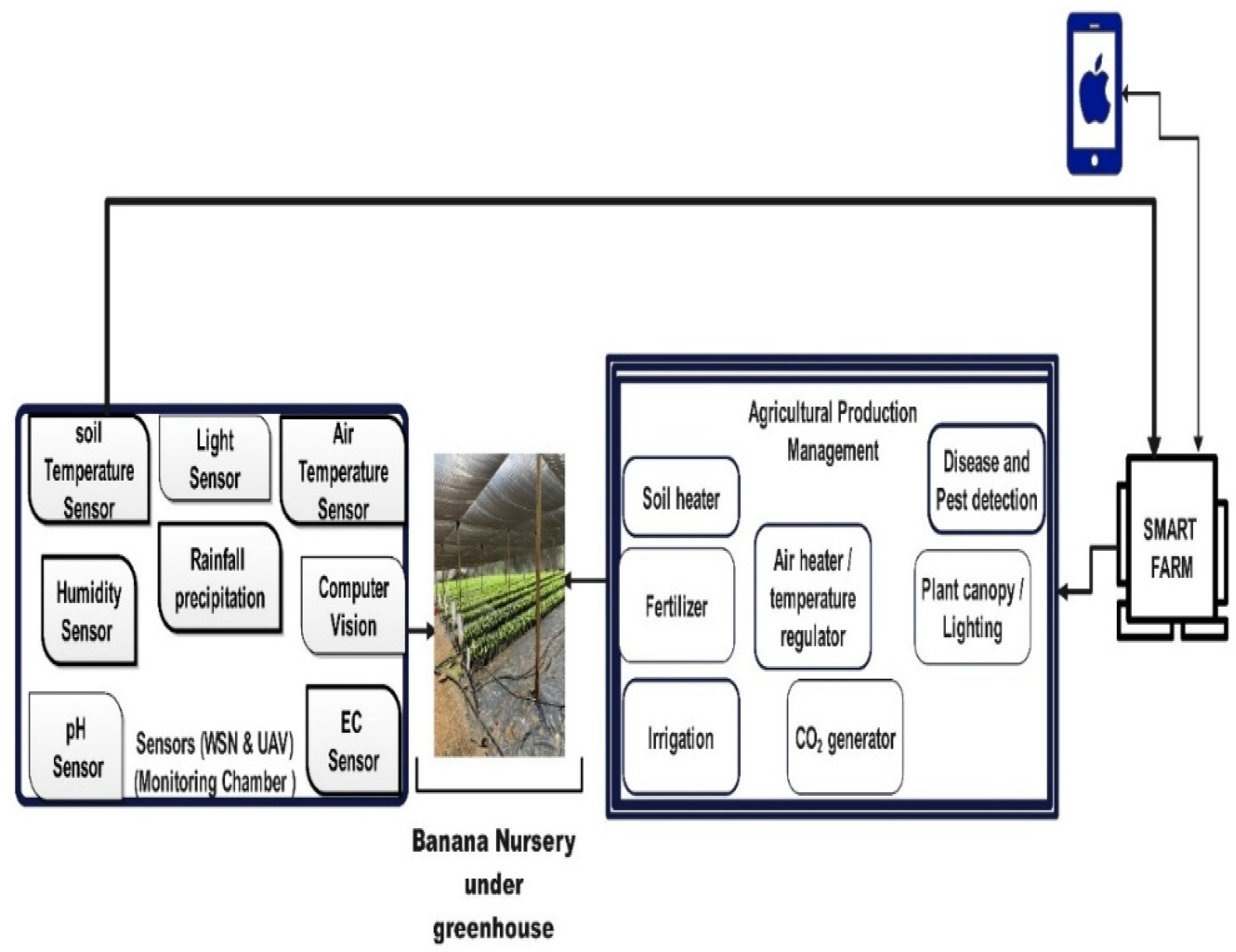
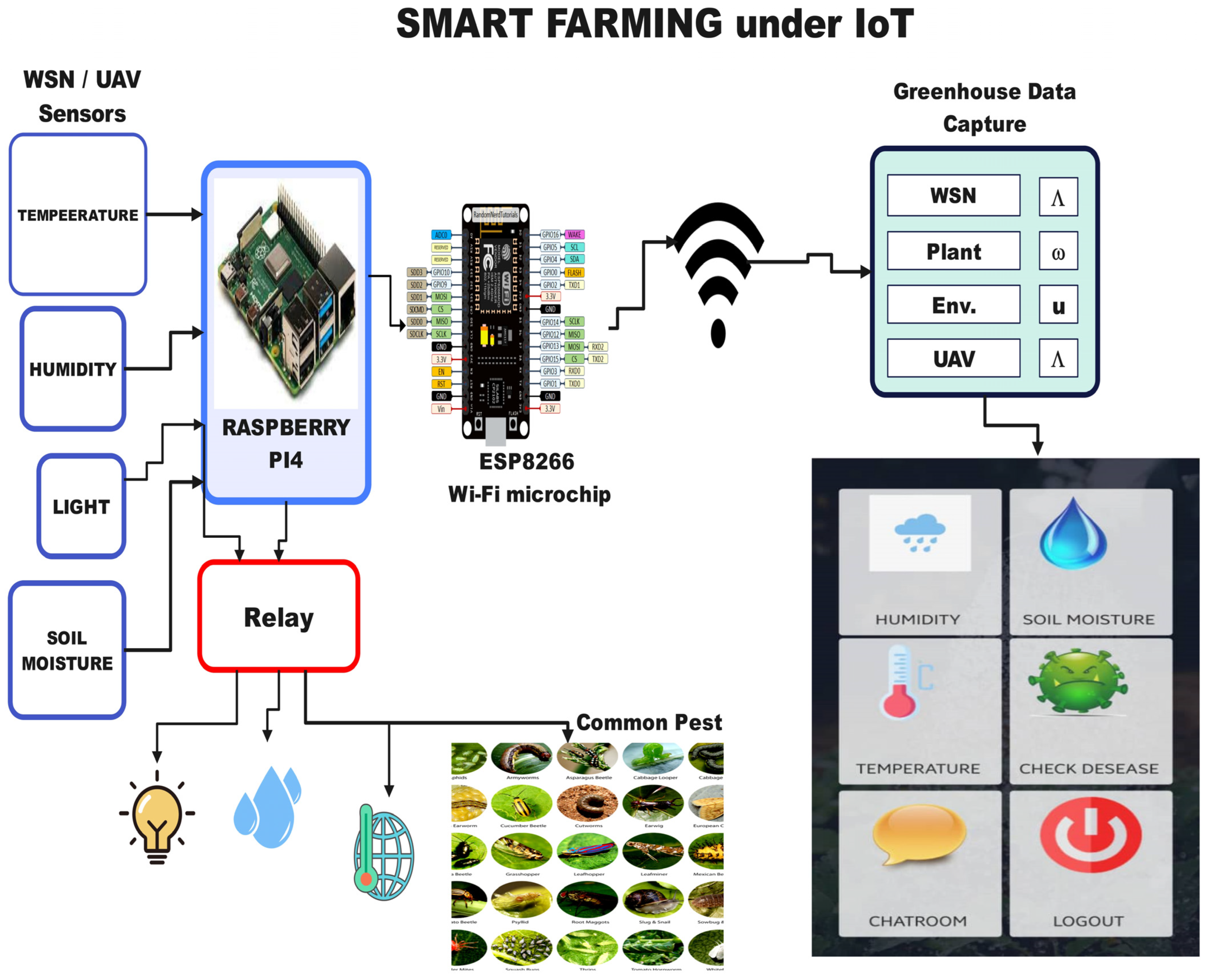
2.2. Technical Details of the SMART FARM Model

SMART FARM outlines a unique implementation of robotic farm monitoring based on the JDL–Mivar model for crop production management. The design philosophy is to mimic an actual crop environment as closely as possible while considering electrical and mechanical limitations. The system is an autonomous, free monitoring, and intelligent farmer call system. The primary function of SMART FARM is to monitor the conditions of crops in a coordinated manner. The most common solution to this requirement is to monitor the temperature (both soil and plant environment), soil pH, soil moisture, and light intensity and duration, as well as to include a weed and disease detection system, irrigation control, and a farmer call and text button, making the design lightweight and convenient. The drone used in this study was DJI Model Number Matric 600, Phantom 4 Pro. This drone is built to carry up to 13 pounds and produce all the thrust needed by relying on six rotor systems, with each being powered by an actively cooled motor [13]. The drone controller was an A3 Flight with six separate batteries that switch on automatically should one fail [13]. The study employs UAVs to provide a preliminary assessment of a potential functional solution for crop weather management and a data fusion system utilising a drone-based meteorological sensor.

The JDL model’s mathematical attributes:

Assuming that the discourse universe for a particular system may be divided into an unknown yet finite number of relevant entities, the challenge of accurately estimating a multi-data world state can be articulated, as seen in Figure 1. In this context, x₁, …, x_k represent entity states, thus transforming the global state estimation problem into identifying the finite collection of entity states ‘X’ that maximises the a posteriori likelihood.

We used the JDL model to find the most likely multi-data state from Figure 1 as

$$\widehat{X}=\arg max\int \lambda \left(X\right)\delta X$$

(1)

$$\widehat{X}=\arg max{\sum }_{k=0}^{\mathrm{\infty }}{\displaystyle \frac{1}{k!}}\int \lambda \left(\left\{X_1,\dots ,X_k\right\}\right)d{X}_1,\dots ,d{X}_k$$

(2)

The challenges in marking the intricacy of the data fusion process are as follows:

(1)

Articulating the uncertainty inherent in observations and in the models of the phenomena that produce these observations.

(2)

Integrating disparate information (e.g., unique characteristics in imagery, weather elements, and signals).

(3)

Managing and processing the vast array of potential associations and interpretations of numerous observations across multiple entities, i.e., UAV and WSN.

It should be noted that the significance of assessing entity states based on context is becoming increasingly evident. A system that amalgamates data association and estimates operations across all levels will enable entities to be comprehended as components of intricate scenarios. A relational analysis, as depicted in Figure 1, allows for the transmission of evidence relevant to a local estimate problem throughout a complicated relational network.

2.3. Information Accumulation Principle

This work utilised the information accumulation principle of two models, JDL and Mivar, to develop an evolutionary data and rules system based on the structure of recorded meteorological variables. This system operates on the foundation of an adaptive, discrete, JDL–Mivar-oriented information space encompassing a single representation of data and rules [14].

The SMART FARM control board receives data from sensors deployed on the farm (WSN) and from the atmosphere (UAV), as well as the present state of the plants identified by computer vision (Figure 2). The control solutions generated by the intelligent farm are sent to the field’s auxiliary systems, where the technological programmes execute the control action. The SMART FARM system utilises the “Raspberry Pi4” as the computing core for logical inference based on the JDL–Mivar model. Users can oversee the condition and administer the system via a mobile and computer software programme. The application programme (APP) and software applications are client–server applications, where the client communicates with the web server using a phone or computer, as specified in Figure 3 and Figure 4, respectively.

Figure 5 illustrates the connection of the sensors to the Raspberry Pi. Most sensors are connected to the GPIO of the Raspberry Pi. Digital sensors can interface directly with the GPIO, whereas analogue sensors must link through an analog-to-digital converter. Supplementary elements, such as minor resistors or capacitors, may be required to constitute the circuit for the sensor. The Rpi.GPIO module for Python enables the reading of sensors attached to the GPIO as indicted in Figure 5 and its display in Figure 4.

2.4. Development of JDL and Attributes from the Fused Data for Greenhouse

This study utilised the most minor discrete information units based on the characteristics of JDL and the Mivar model [16]. The fundamental components of the Wireless Sensor Network (WSN) and the Unmanned Aerial Vehicle (UAV) were the sensor nodes, and connections were established between sensors. The JDL–Mivar model represents a collection of axes, elements, space points, and field data values recorded in compatible units.

$$\wedge =\left\{{\alpha }_n\right\},n=1,\dots ,N,$$

(3)

where ‘ᴧ’ is the set of Mivar space axis names adopted from [17], and ‘N’ is the number of Mivar space axes. Equation (3) can then be written as

$$\bigvee {\alpha }_n\exists {\mathcal{F}}_n=\left\{f_{n{i}_n}\right\},n=1,\dots ,I_n$$

(4)

where ‘Ƒn’ is a set of axis ‘αn’ elements, ‘in’ is a set of ‘Ƒn’ elements, ‘In’ = |‘Ƒn’ |, and ‘Ƒn’ sets form multi-sensor readings.

Now, introducing the JDL model equation into the Mivar equation results in the following:

$$\mathsf{\Lambda }={\sum }_{i=1}^{m}log\left[{\displaystyle \frac{p_{di}\mathrm{e}\mathrm{x}\mathrm{p}\{-(z_i-h_i{)}^2/2{\sigma }^2\}+\left(1-p_{di}\right)\mathrm{e}\mathrm{x}\mathrm{p}\{-(z_i+h_i{)}^2/2{\sigma }^2\}}{p_{fai}\mathrm{e}\mathrm{x}\mathrm{p}\{-(z_i-h_i{)}^2/2{\sigma }^2\}+\left(1-p_{fai}\right)\mathrm{e}\mathrm{x}\mathrm{p}\{-(z_i+h_i{)}^2/2{\sigma }^2\}}}\right]JDL$$

(5)

adding

$$\wedge =\left\{{\alpha }_n\right\},n=1,\dots ,N,$$

(6)

$$\bigvee {\alpha }_n\exists {\mathcal{F}}_n=\left\{f_{n{i}_n}\right\},n=1,\dots ,I_{n}Mivar$$

(7)

The joint JDL–Mivar model for crop management then becomes

$$\mathsf{\Lambda }={\sum }_{i=1}^{m}log\left[{\displaystyle \frac{p_{di}\mathrm{e}\mathrm{x}\mathrm{p}\{-(z_i-h_i{)}^2/2{\sigma }^2\}+\left(1-p_{di}\right)\mathrm{e}\mathrm{x}\mathrm{p}\{-(z_i+h_i{)}^2/2{\sigma }^2\}}{p_{fai}\mathrm{e}\mathrm{x}\mathrm{p}\{-(z_i-h_i{)}^2/2{\sigma }^2\}+\left(1-p_{fai}\right)\mathrm{e}\mathrm{x}\mathrm{p}\{-(z_i+h_i{)}^2/2{\sigma }^2\}}}\right]+\left\{{\alpha }_n\right\},n=1,\dots ,N,$$

(8)

where ‘Λ’ is the central fusion station (CFS), pdi is the sum of soil conditions measured, ‘zi’ is the data received from WSN sensors, ‘m’ is the number of sensors deployed, ‘hi’ is the received data from the UAV as the channel, ‘pfai’ is the data aggregator for elements of the same identity, and ‘σ‘ is the received energy from the sensors.

The obtained equation is now entered into computer programming software (the python platform (Python 3.12.8 ) to calculate the resultant parameters of interest. Describing the interconnections of modelling becomes complex due to a diverse set of capabilities, yet it can account for all relevant elements. The Mivar and JDL computations employ mathematical logic to function well in crop management. The integration of the JDL–Mivar model enables the compelling depiction [18] of sensor node characteristics obtained from the field and facilitates the dissemination and advancement of these characteristics across several layers. This potent methodology can be utilised in many domains within the agricultural value chain.

Formally, we address a time-series issue with inputs containing multivariate time-series together with potential metadata [19], where the goal is to develop a function that reliably predicts the output. The fusion method simultaneously considers the complete array of sensors and their associated predictors, resulting in an expanded dataset. The fusion jointly estimates the parameters from all available time-series (or sensors) in the greenhouse, depicting the scenarios in the previous chapters of the study (

Table 1. Summary of variables incorporated in the fusion model, detailing their classification and a concise description for greenhouse irrigation.

Variable	Type	Description	Included in JDL Model
Fused Dataset (‘ꝩ1’)-(Soil water potential)	Target	First-order difference in daily average soil water potential values for a specific plot and year at a specific depth	x
Plant Name (Banana)	Static categorical	Plant name differentiates between plants and characteristics	x
Soil texture	Static categorical	Texture of the soil	x
Pruning treatment	Static categorical	Weather leaves or roots were pruned	x
Irrigation treatment	Static categorical	Whether deficit irrigation was applied or not	x
Sensor depth	Static real	Depth of the soil moisture sensor in cm	x
Soil water potential centre	Static real	Mean of the soil water potential input window	x
Soil water potential scale	Static real	Scale of the soil water potential input window	x
Measurement year	Static real	Measurement year	x
Measurement month	Known categorical	Measurement month	x
Relative time index	Known real	Time index (in days) since k	x
Precipitation	Known real	Daily total precipitation	x
Reference evapotranspiration	Known real	Reference evapotranspiration (ETo), which is the same for all fields here	x
‘ꝩ1’-(Soil water potential)	Historic real	History of the target	x
Irrigation amount	Historic real	Amount of irrigation applied to a specific plot	x
Humidity	Historic real	Daily Humidity	x
Soil temperature	Historic real	Daily mean soil temperature around soil moisture sensor (measured by soil moisture sensor)	x
Reference evapotranspiration	Historic real	Reference evapotranspiration (ETo)	x

). Consequently, neural networks have demonstrated significant potential as fusion forecasters due to their efficacy in extensive data environments. Indeed, with sufficient data, fusion forecasting techniques like neural networks can intrinsically represent more intricate non-linear patterns in the data than local methods, which are constrained by their reliance solely on localised data. In an agricultural context, this enables the conditioning of field-specific, time-invariant variables, facilitating efficient data fusion across various static features. JDL utilises a sophisticated architecture that enables the modelling of intricate interactions among various temporal (future or historical) and static inputs while maintaining interpretability. The practical implications of our findings are substantial in smart agriculture.

The sophisticated forecasting skills of the JDL model may result in more effective and sustainable irrigation strategies customised to the unique requirements of banana cultivation. This will facilitate the optimisation of water utilisation and assist farmers in making informed decisions.

2.5. Rules for Irrigation Activation

Rule 1

||Whenever the time is 6:53 a.m.

and the month is later than October, and the month is earlier than December.

and the day(s) of the week is/are S-T-T-S

then activate the water field (task 1)

Rule 2

||Whenever water on the field (task 1) is activated,

and output 205 states is off,

then turn the first field (out 11) on for 10 min.

Rule 3

||Whenever the first field (out of 11) state is turned off,

and output 205 states is off,

then turn the second field (out 12) on for 10 min.

Rule 4

||Turn off the irrigation and set a flag if the rain or moisture sensor is triggered.

Whenever disable drip (task 2) is activated,

Then turn output 205 on

Then turn the first field (out 11) off,

Then turn the second (out 12) off,

Rule 5

||Reset irrigation zone output if no rain or moisture is detected today.

whenever the time is 12:00 am

and rain or moisture sensor (zn 15) is secure,

then turn output 205 off,

||Var Moisture, last_activation, frequency, y, ris, cur_h;

||IF (moisture < 35.5 &&

(last_activation >= frequency | last_activation = −1) {

if(cur_h >= ris && cur_h< ris +2) {

y = “Activate”;

}

||ELSE {

y = “Forbid”;

}

}

else {y = “Forbid”;}

The flowchart (Figure 6) commences with the initialisation of a path and a set of visited or captured sensors. It verifies whether the current sensor node is the objective. If affirmative, it returns the path; if not, it investigates the designated nodes, organises them, and chooses the subsequent node. If a node is visited or captured, it is omitted. This flowchart was utilised in the pathfinding algorithms and data navigation systems. The crop management dashboard enables farmers and businesses to leverage real-time data to benefit individuals across the organisation through interactive dashboards and apps that everyone can access. The API data experience platform is built on a safe, adaptable data foundation that connects several data systems. For example, by applying Nitrogen (N), Phosphorus (P) and Potassium (K) (NPK), farmers can progress from basic charts and graphs to data experiences that pique interest, power insights and action, and give exponential results based on plant nutrient requirements.

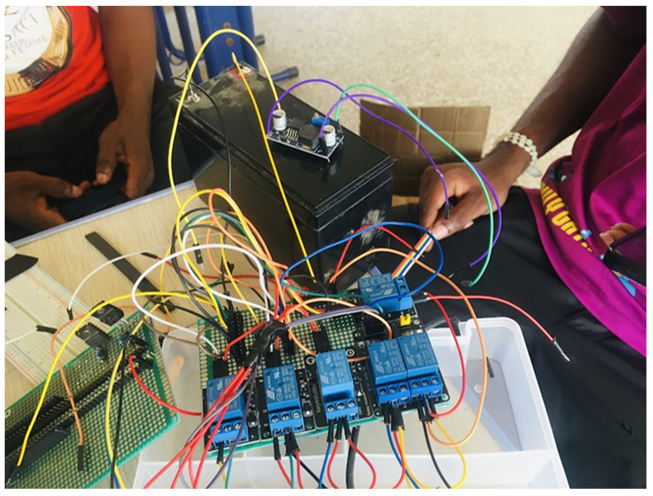
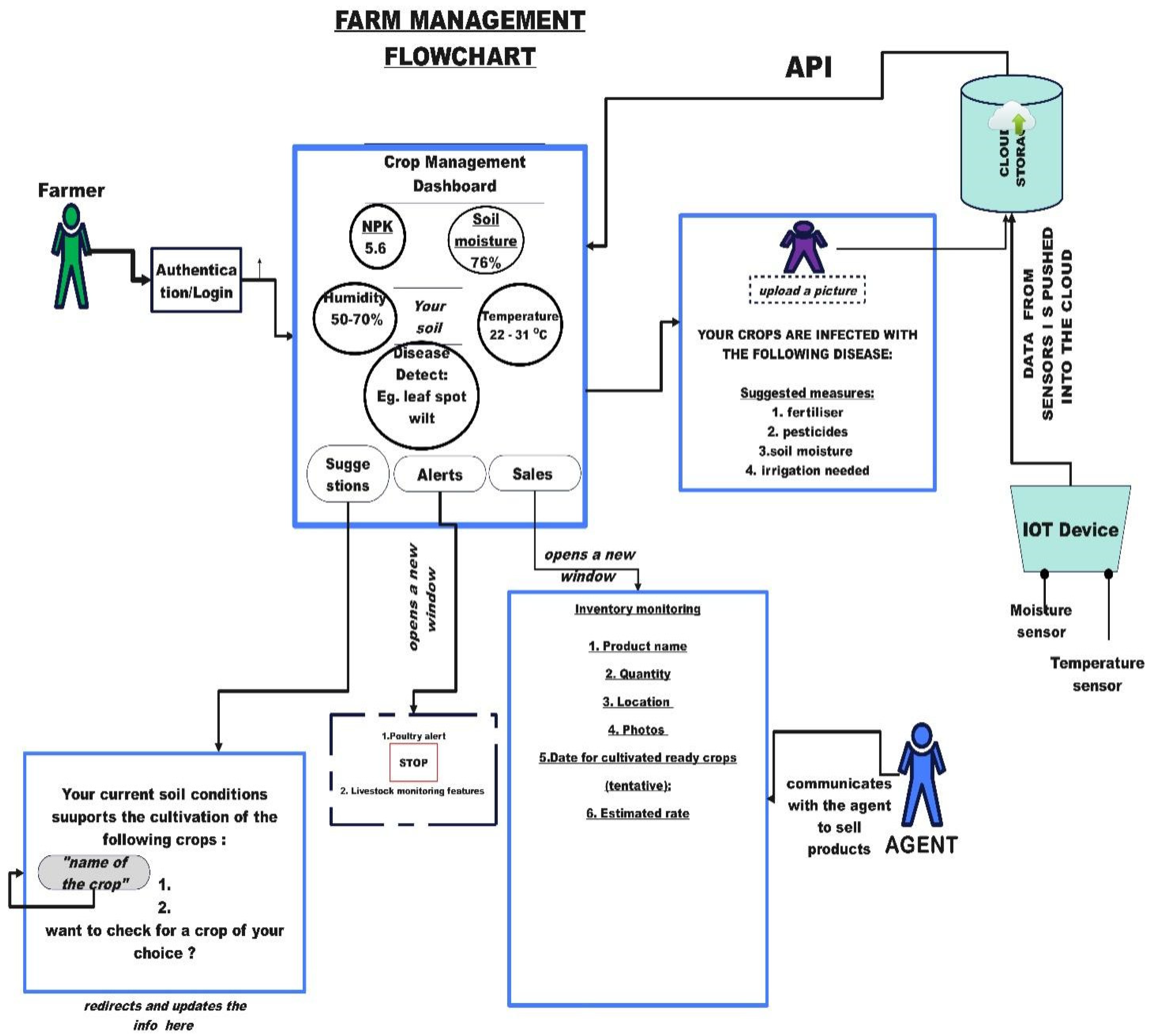
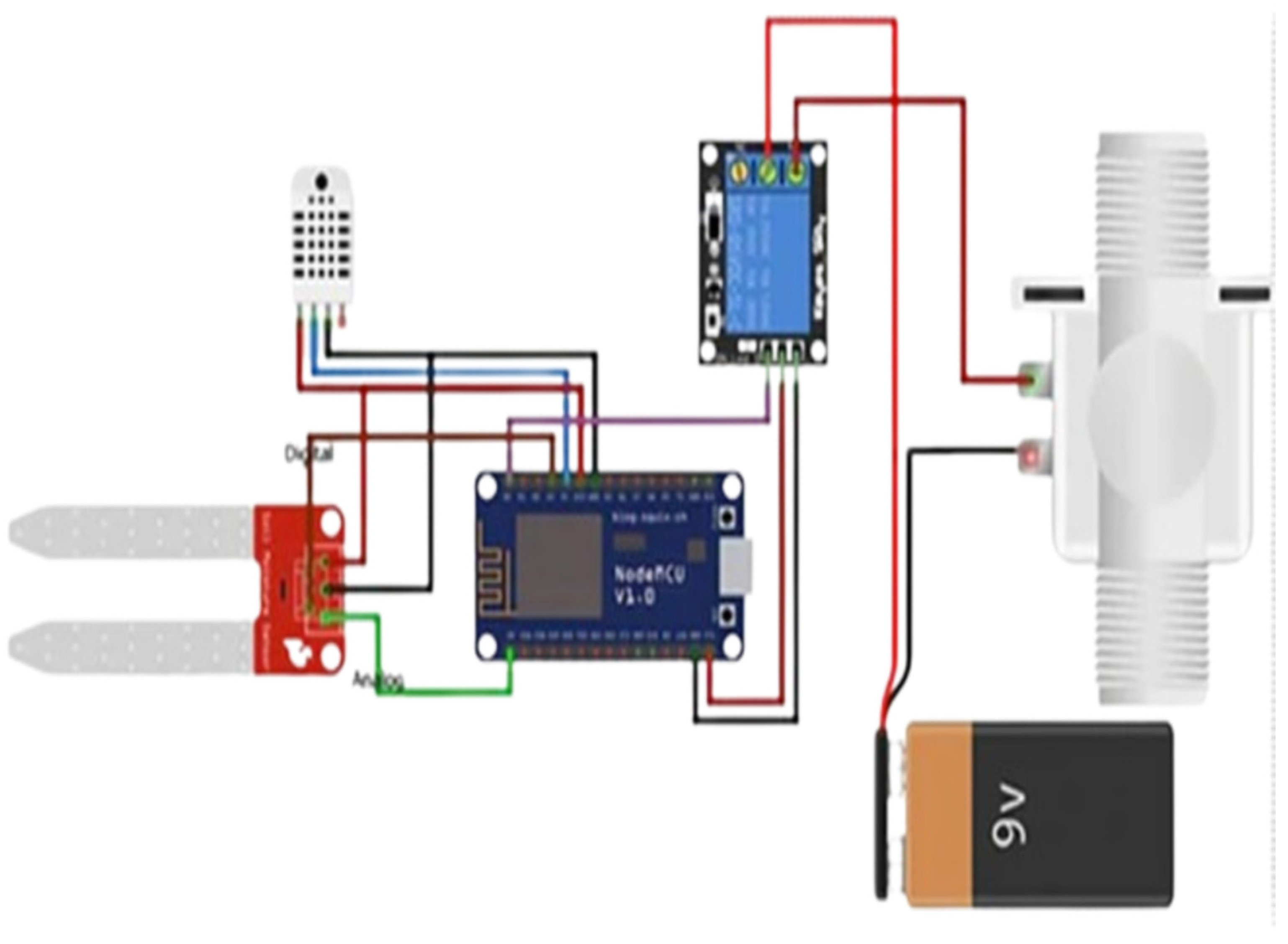
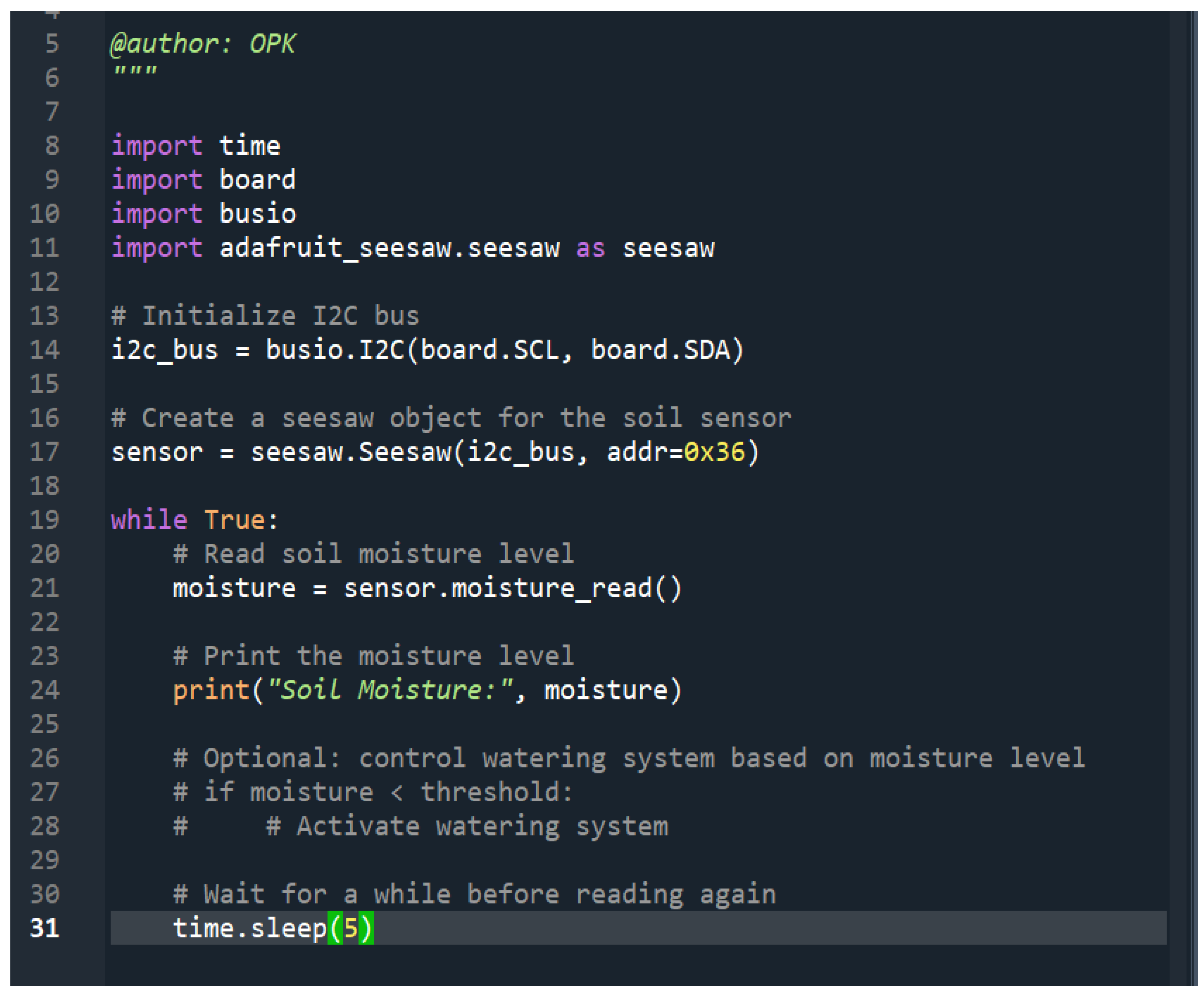
2.6. Building a Prototype and Crop Management Flow

The necessary components for intelligent plant monitoring are as follows:

The hardware utilised in the project included NodeMCU ESP8266, a soil moisture sensor, a temperature and humidity sensor, a relay module, and a water pump. The project utilised Arduino IDE for programming the ESP8266 NodeMCU board and the SMART FARM app for IoT control and wireless monitoring.

The soil moisture sensor is connected to the NodeMCU’s A0 analogue pin based on the algorithm flow chart in Figure 7. The flowchart was used to determine the irrigation patterns and how the sensors send signal to the main control board. In Figure 8, the NodeMCU’s D4 pin, which is a digital pin, is connected to the signal pin of the DHT temperature and humidity sensor. The relay module is connected to the NodeMCU’s D5 pin.

The water pump is additionally connected to the engine. The NodeMCU’s D3 pin is connected to the LED. This functions as a nocturnal source of light for IoT-managed nighttime operations. The NodeMCU consistently receives an analogue signal from the DHT and moisture sensors, which it subsequently utilises to validate the temperature, humidity, and moisture levels. The crop management flow structure is as follows:

(1) The components should be interconnected according to the layout depicted in the circuit diagram. Install the Blynk application on your smartphone and select the option to create a new project.

(2) Choose the NodeMCU board and click the Create button. Install three gauges visually representing temperature, humidity, and soil moisture levels.

(3) Soil moisture refers to the amount of water in the soil. Configure the Virtual two pin (V2) with a value range of 0–200 and set the time interval to 1 s. Repeat the same process for the temperature (V6) and humidity (V5). Include a button and a timer.

(4) Access the button’s settings and modify its name to ‘Water’. Choose digital pin 0 (D0) and pick the switch by sliding the point to switch from push.

(5) Access the timer’s settings and choose the option labelled ‘D0’. We can establish the specific times that the motor, namely the relay, can be turned on and off. After properly selecting the appropriate board and port on the Arduino IDE, upload the code into the board.

The programming of sensors using Python 3.12.8 is primarily contingent upon the specific sensor type and the microcontroller employed. This study used a capacitive soil moisture sensor with a Raspberry Pi, NodeMCU and the Adafruit Circuit Python library (Figure 9).

3. Results

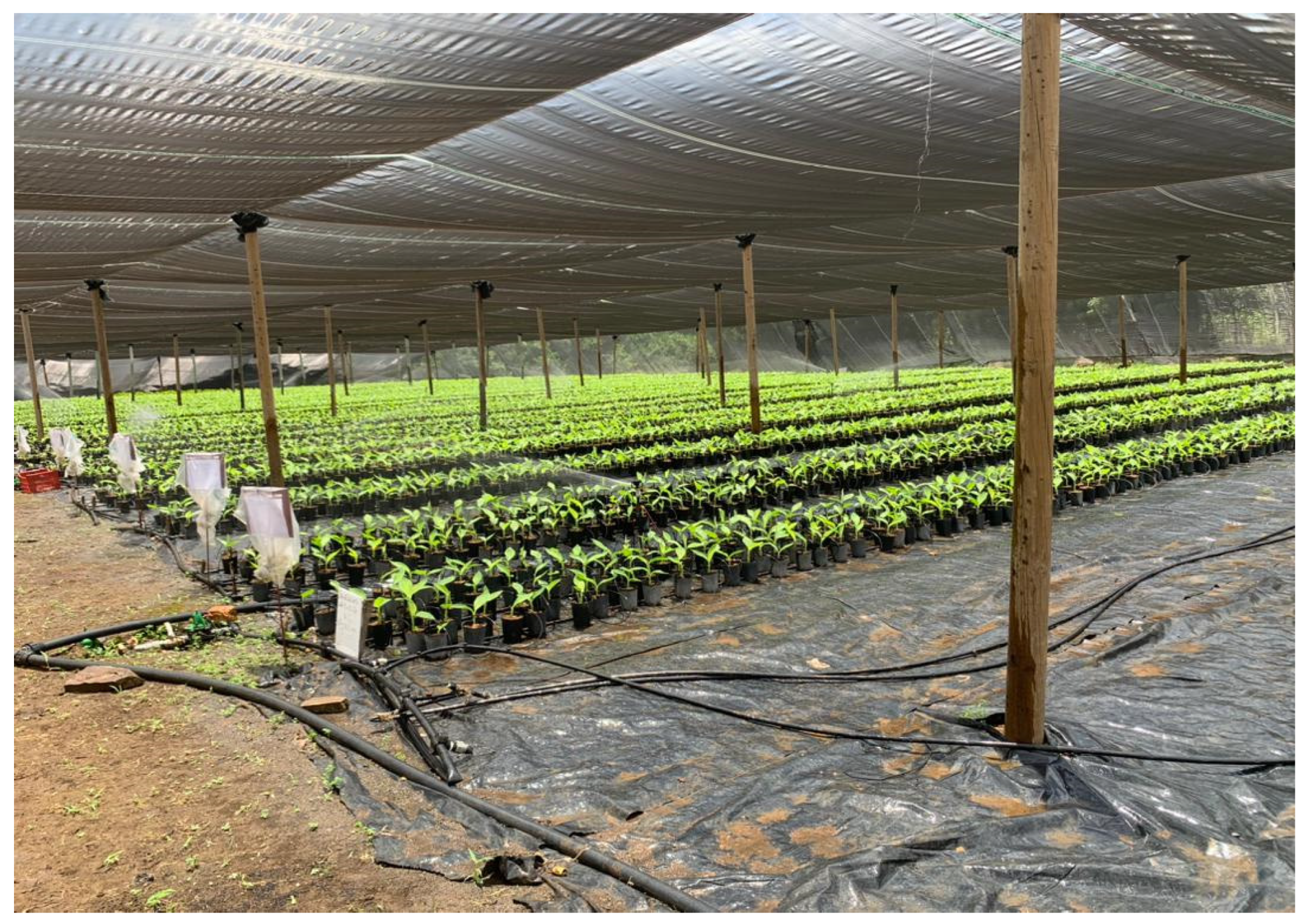
3.1. Operation of the Model and the System

The primary objective of the plant moisture monitoring system is to mechanise the process of monitoring and irrigating plants using a variety of sensors and a microprocessor. The system utilises the NodeMCU ESP8266 (produced by Espressif Systems in Shanghai, China) as the primary controller, which establishes a connection to Wi-Fi for remote monitoring capabilities.

The soil moisture sensor quantifies the soil’s moisture content, enabling us to ascertain whether the plant needs irrigation or any other form of assistance. Temperature and humidity sensors, as implied by their names, quantify the prevailing environmental conditions. These elements are equally significant for crop expansion. The relay module regulates the water pump and guarantees an adequate water supply for the plant’s development.

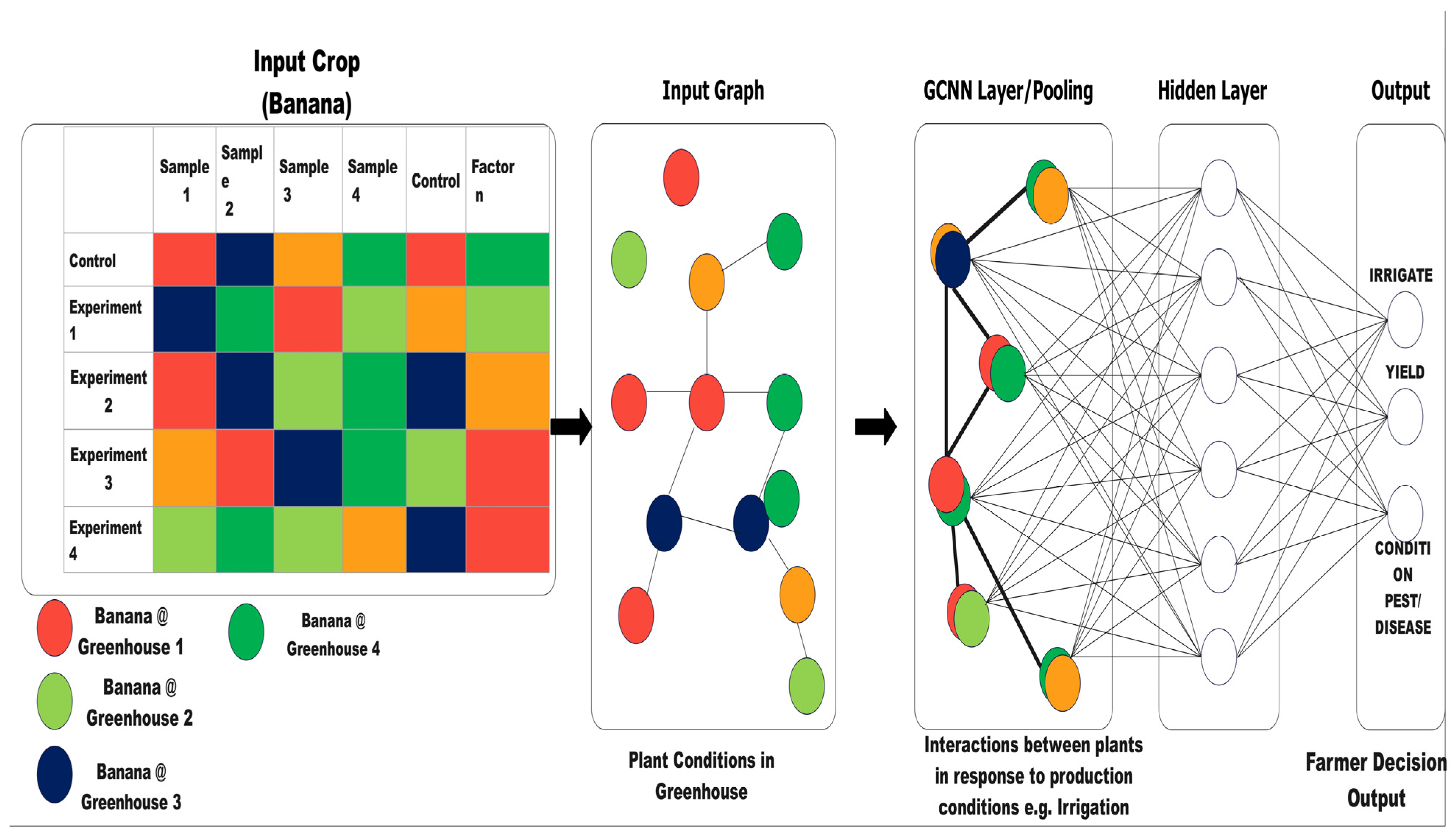
3.2. JDL Network for Banana via Morphological Image Processing

The research developed a convolutional neural network using sensors to survey the soil conditions and vegetation. Initially, we amassed a substantial dataset from soil sensor readings, preprocessed the data into an appropriate format, and devised a CNN architecture incorporating convolutional layers to extract characteristics from the data.

Subsequently, we trained the model utilising JDL fusion techniques on the data and employed the trained model to forecast soil conditions based on the sensor readings. The essential phases encompassed data collection, data preparation, selection of a suitable CNN architecture, training, and evaluation. The use of algorithms based on an active trainable evolutionary JDL–Mivar network enables the implementation of a plant care system that considers the specific characteristics of crop growth, makes decisions in the presence of diverse sensor data, and promptly adjusts the plant growth process. The study employed a JDL model and CNN algorithms to identify banana plants’ irrigation (water) requirements and stress levels in a greenhouse setting. The study utilised a multi-step approach to analyse water stress patterns efficiently, leveraging picture segmentation and morphological image processing techniques. The greenhouse has a dimension range of 4500 square feet. Initially, there was an issue with processing extensive UAV banana imagery. To resolve this issue, we partitioned the large-scale UAV banana picture into smaller segments using OpenCV in Python [21], resulting in 6832 images for each sampling date (Figure 10 illustrates the obtained dataset). The new image’s dimensions were 64 × 64 × 3 (width, height, depth).

The irrigation treatment constituted the ground truth, which is also included at the bottom of each image in Figure 10 for illustration. The objective was to employ the CNN model to train the image dataset and categorise the images into one of the four irrigation regimes. The phrase “ground truth” is essential in supervised machine learning activities like picture categorisation. It denotes the established and validated proper responses or labels for the data utilised in the training and evaluation of machine learning models. With this ground truth information, the CNN model may learn from examples and enhance its capacity to classify images into designated categories accurately. We initially divided the extensive UAV banana image into smaller segments using OpenCV, resulting in 6832 images for each sampling date. To investigate the impact of elements on water stress prediction, including canopy and soil features, we employed morphological image processing techniques utilising sci-kit-image, an image processing library in Python.

Morphological image processing is a crucial method for analysing and modifying images according to their shape and structure [22]. It is based on mathematical morphology, which offers a collection of operations for extracting, improving, and altering the geometric features found in an image. These procedures are fundamentally grounded in the principles of dilation, erosion, opening, and shutting [22]. Dilation enlarges the shape’s limits and fills voids, whereas erosion diminishes the boundaries and eliminates minor details.

The opening process entails erosion, which is succeeded by dilatation and eliminating noise and minor objects. Conversely, closure entails a sequence of dilation succeeded by erosion, effective for bridging gaps and uniting fragmented structures [22]. Morphological image processing techniques facilitate the extraction of significant features, elimination of noise, segmentation of objects, and execution of other critical image analysis tasks, hence enhancing the interpretation and comprehension of the banana image.

By delineating the image into banana and soil regions [23], we could examine each location’s unique qualities and attributes. This method facilitated an extensive examination of the manifestation of water stress in the banana canopy compared to the soil, yielding significant insights into the determinants of water availability and distribution inside the greenhouse.

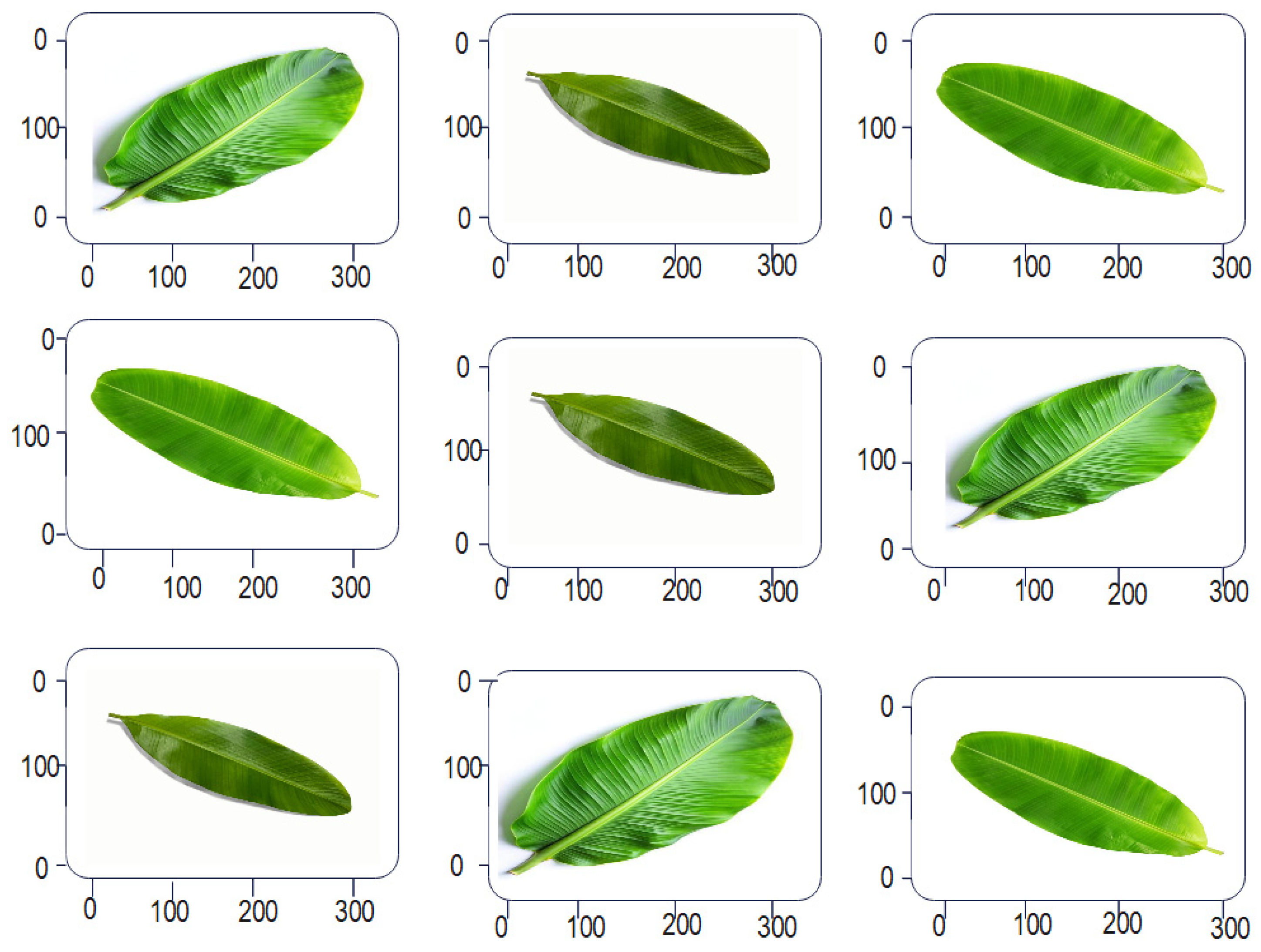
3.3. Image Processing for the CNN Model, Banana Leaf, and Canopy Analysis

During the data preprocessing phase, the authors segmented the extensive UAV banana photos into smaller scales, yielding 6832 images for each sampling day.

To establish a training and testing dataset, the UAV dataset was divided into 70% for training and 30% for testing. We generated a network illustrating the first 25 photos from the training set, with the respective class names indicated beneath each image (Figure 11). The CNN model was implemented using the TensorFlow 2.0 framework [24].

The architecture of the CNN model is defined in Table 1 and Figure 11. The model predominantly comprised Conv2D and MaxPooling2D layers, generating a 3D tensor output representing height, width, and channels. The width and height measurements generally diminished as the network progressed more profoundly. The number of output channels for each Conv2D layer was dictated by the first argument provided. The output tensor produced by the convolutional base was subsequently input into dense layers for classification. The dataset had four irrigation treatments, resulting in the final dense layer having four outputs, which allowed the model to categorise the input photos into the corresponding treatment classifications. This architecture enabled the model to learn and differentiate among the various irrigation treatments based on the supplied training data.

Parameter tuning is an essential phase in constructing the CNN model since it entails identifying the ideal configuration of hyperparameters to improve the model’s performance. Hyperparameters are external settings that cannot be derived from the data and profoundly affect the model’s performance. In the context of the CNN model, hyperparameters encompass values such as the number of neurones in layers, kernel sizes in convolutional layers, and the selection of optimiser methods.

Automated tools, libraries, and frameworks, such as sci-kit-learn and TensorFlow, provide systematic hyperparameter tuning [25], enhancing the accuracy and robustness of machine learning and deep learning models. This article examined settings inside the following grid: {‘optimizer’: [‘adam’, ‘sgd’], ‘neurons’: [32, 64, 128], ‘kernel_size’: [(3, 3), (4, 4)], ‘pool_size’: [(2, 2), (3, 3)]}. The architecture presented in

Table 2. The CNN model architecture.

Layer Type	Output Shape	Parameter Numbers
Conv2D	(None, 62, 62, 32)	896
MaxPooling2D	(None, 31, 31, 32)	0
Conv2D	(None, 29, 29, 64)	18,496
MaxPooling2D	(None, 14, 14, 64)	0
Conv2D	(None, 12, 12, 64)	36,928
Flatten	(None, 9216)	0
Dense	(None, 64)	589,888
Dense	(None, 4)	260

exhibited the optimal model performance for our validation. The CNN model employed in this study can be readily replicated for validation purposes.

Convolutional neural networks (CNNs) constitute the fundamental architecture for most deep learning algorithms used in image recognition [26]. The essential structure is seen in Figure 11. The focus of Figure 11 is to streamline the structure of data, enhance training efficiency, and facilitate deeper training layers. To simplify the CNN neural network for data processing, we employed strategies such as refining the model architecture (utilising efficient convolutional layers and minimising network depth). We augmented the data to enhance variability, tuning hyperparameters to identify optimal learning rate and batch size.

We again pruned the network to eliminate superfluous connections, quantising to decrease the model size, and applied knowledge distillation to convey insights from a larger model to a more compact one. This strategy was applied while assessing performance to ensure that accuracy remains intact. The experimental stages were depicted as Experiment 1 (fully irrigated); Experiment 2 (percent deficit); Experiment 3 (irrigation time delay); and Experiment 4 (fully irrigated) as shown in Figure 11.

Patrignani [26,27] states that canopy cover is generally measured as the percentage of ground area obscured by the vertical projection of the plant canopy. This metric is intricately linked to crop growth, development, water usage, and photosynthesis, making it a crucial attribute that requires ongoing monitoring during the growing season [27]. Assessing banana canopy cover throughout the growing season might yield significant insights into the banana’s overall performance. To thoroughly comprehend banana growth during the 2023 growing season, the authors examined canopy cover trends, a crucial sign of banana development. The canopy cover was determined using the methodology outlined in the research by Bastow et al. [28].

The RGB Ortho mosaic image was initially categorised into a binary map via the Canopeo technique [29]. Subsequently, Equations (9) and (10) were utilised to calculate the canopy cove:

$$Canopy=\left({\displaystyle \frac{red}{green}}<p_1\right)and\left({\displaystyle \frac{blue}{green}}<p_2\right)and(2green-blue-red>p_3$$

(9)

The corresponding band’s pixel values are red, green, and blue. The parameters p₁, p₂, and p₃ classify pixels predominantly in the green band {37, 38}. The adopted values for the Canopeo algorithm are p₁ = 0.95, p₂ = 0.95, and p₃ = 20.

$$CanopyCover\left(\%\right)={\displaystyle \frac{\Sigma \left(CanopyAreainImage\right)}{\Sigma \left(TotalImageArea\right)}}\times 10$$

(10)

Canopy Cover (%) = (Canopy Area in Image/Total Image Area) × 100

where canopy cover estimation is based on the Hemispherical Photography Method [29].

In the feature importance analysis, the random forest classifier was trained on an identical dataset utilised for training the CNN model (the dataset from 20 June 2022).

The random forest algorithm is a robust machine learning method that offers insights into the significance of various input variables for precise predictions. It generates numerous decision trees and averages their predictions to yield a final categorisation outcome. This investigation evaluates the influence of each feature on the decrease in impurity in decision trees. The default configuration of ‘sklearn.ensemble.RandomForestClassifier’ from sci-kit-learn was utilised for feature significance analysis in the random forest technique. The code is included in the appendix, where parameters are displayed using the ‘RandomForestClassifier().get_params()’ function [30].

In contrast to ‘activation maps’ or ‘gradient-based’ approaches, employing a random forest for feature significance analysis is especially advantageous when interpretability and transparency are paramount. Conversely, ‘activation maps’ and ‘gradient-based’ techniques frequently entail intricate calculations and may yield fewer clear interpretations of feature significance. Random forest offers a highly interpretable method for evaluating feature relevance. Collecting decision trees facilitates a comprehensive understanding of each feature’s contribution to the overall forecast. Although activation maps or gradient-based techniques can elucidate which areas of the input influence the output, their interpretation may lack the intuitiveness of the feature importance scores generated by random forests. Consequently, feature significance analysis utilising the random forest method is favoured for assessing banana water stress in this study.

The SMART FARM data recorder monitors various soil and plant parameters using smart sensors. It provides remote wireless monitoring for accurate soil and plant conditions, enhancing the understanding of banana cultivation in the greenhouse (Figure 12). In the banana water stress test, eight features were extracted from the UAV-based RGB image: “red”, “green”, “blue”, “exgreenness”, “canopy cover”, “canopy volume”, “mask size”, and “canopy height”. The “red”, “green”, and “blue” represent the average band reflectance values for the banana canopy region. The term “exgreeness” denotes the Excess Green Index (EXGI). The EXGI differentiates the green segment of the spectrum from red and blue to identify vegetation vs. soil and can also be utilised to forecast NDVI values.

It has demonstrated superior performance to other indices utilising the visible spectrum for vegetation differentiation. The EXGI was calculated using Equation (11) [31]:

$$EXGI=2G-(R+B)$$

(11)

G, R, and B are normalised green, red, and blue bands.

The canopy volume was then calculated from Equation (11);

$$canopyvolume=\Sigma (H_i\times GS{D}^2)$$

(12)

where ‘H_i’ represents the height of the ‘i^th’ pixel.

The CHM (canopy height model) computed the canopy height calculation. The CHM is generated by subtracting the DSM (digital surface model) of each flight from the digital terrain model (DTM) obtained from the first flight.

The first flight was conducted after transplanting into the greenhouse and prior to the emergence of the third leaf to obtain the greenhouse ground surface.

3.4. Overall Banana Growth Trend in the Greenhouse

The irrigation treatment significantly influenced banana development, and its effect on canopy cover was assessed according to the quantity, frequency, and timing of water delivery (Figure 13).

Irrigated plants resulted in excessive canopy cover, as they responded to adequate water availability by generating additional leaves. Consequently, according to the individual plant water needs, administering water in the correct quantity and time is essential for attaining optimal canopy coverage and fostering robust plant growth.

Irrigation treatments played a vital role in banana growth, and their impact on the plant’s canopy cover was evaluated based on the amount, frequency, and timing of water application. Significantly, a key research finding was the considerable disparities among the irrigation treatments throughout the latter phases of the growing season, particularly between 150 and 200 days post-emergence of the third leaf (Figure 13).

This period signified a pivotal phase in which the varying impacts of distinct irrigation regimes on canopy cover were increasingly evident. Comprehending these differences and their consequences during this timeframe yielded significant insights into the appropriate management of irrigation practises for greenhouse banana growth. Given the significance of this phase, the following element of the study mainly concentrated on employing the dataset gathered for training and evaluating the CNN models. Focusing on this timeframe, we sought to identify and examine the essential characteristics and trends associated with banana growth that manifested throughout these pivotal months. This focused methodology facilitated a comprehensive examination of the impact of irrigation treatments on banana growth and yielded significant data for the training and assessment of the CNN models.

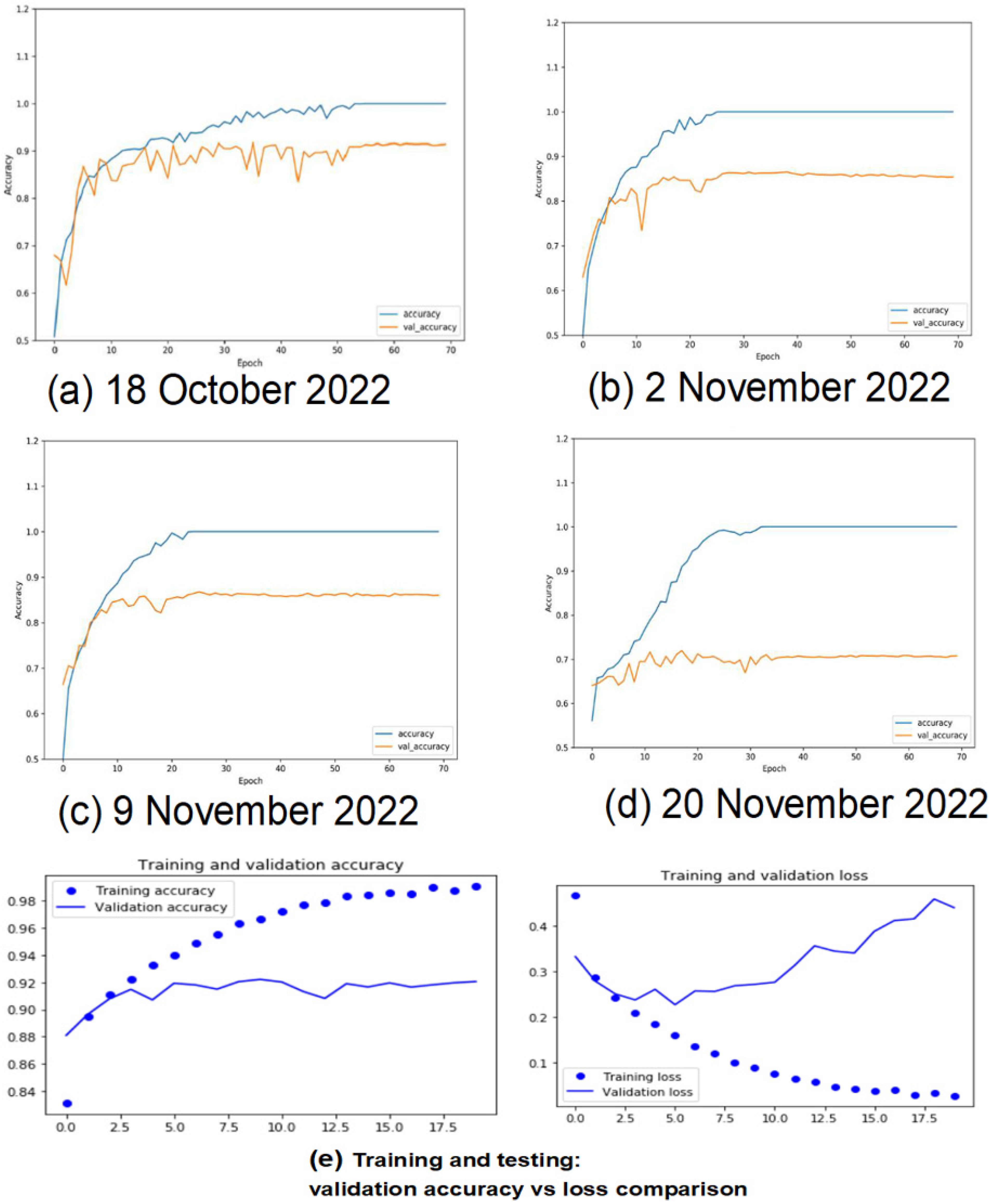
3.5. The CNN Model’s Performance

The CNN model utilises an input image of the banana leaf (Figure 10), represented as a tensor with dimensions of height, width, and channels, where each channel corresponds to a colour component: red, green, and blue. The model’s output is the prediction of banana water stress levels. This consists of predictions and classification labels derived from information retrieved from the image via convolutional layers, typically culminating in a probability distribution across various classes.

The CNN model receives an image as input and produces a prediction regarding its content. The research employed 6832 banana canopy pictures for each sampling date: 18 October, 2 November, 9 November, and 20 November, all in 2022.

The dataset was randomly divided into a 70% training set and a 30% testing set on each sample day. During the training process, the CNN model was trained via the “Adam” optimiser and the cross-entropy loss function. The model underwent training for 70 epochs to enhance its performance. To evaluate the efficacy of the trained CNN models, we utilised the original dataset and illustrated the training and testing accuracy trajectories as the number of epochs escalated (Figure 14). The test accuracy fluctuated throughout sampling dates, recording roughly 91% on 18 October, 86% on 2 November, 87% on 9 November, and 70% on 20 November in 2022.

The accuracy ratings offered insights into the performance of the CNN models in identifying banana water stress levels across several sampling dates. Figure 14e indicates that the validation accuracy plateaued after 4–5 epochs, with infrequent increases at specific epochs. The validation accuracy initially exhibited a linear growth with the loss; however, it plateaued with minimal improvement. The validation loss indicates overfitting since it initially declined linearly like the validation accuracy but began to rise after 4–5 epochs. This suggests that the model attempted to memorise the data and was successful. Precision and recall values were computed and are detailed in Table 2 to elucidate the model’s performance. Precision quantifies the ratio of accurately predicted instances for each class, whereas recall quantifies the ratio of accurately predicted cases relative to the total instances of a specific class.

These measurements offer significant insights into the model’s precision and capacity to classify various irrigation treatment amounts accurately. The test accuracy fluctuated by sampling date, reaching roughly 91% on 18 October, 86% on 2 November, 87% on 9 November, and 70% on 20 November in 2022. The diminished performance noted on the most recent sampling date (20 November) was the outcome of data drift due to changes in the data distribution over time, which reduced the performance of the model; so, gathering more data and applying batch normalising and layer normalising data augmentation methods stabilised the training and helped to fix this problem.

From

Table 3. The CNN model’s classification performance on irrigation treatments against leaf development with sampling dates.

Sample Date	Irrigation Treatments	Precision	Recall	F1-Score
18 October	Fully irrigated	0.92	0.93	0.93
18 October	percent deficit	0.89	0.92	0.90
18 October	Irrigation time delay	0.90	0.88	0.89
2 November	Fully irrigated	0.83	0.83	0.83
2 November	percent deficit	0.82	0.84	0.83
2 November	Irrigation time delay	0.83	0.81	0.82
9 November	Fully irrigated	0.84	0.83	0.84
9 November	per cent deficit	0.84	0.85	0.84
9 November	Irrigation time delay	0.81	0.81	0.81
20 November	Fully irrigated	0.83	0.82	0.82
20 November	per cent deficit	0.60	0.63	0.62
20 November	Irrigation time delay	0.60	0.56	0.58

, the CNN model exhibits exceptional performance in classifying banana water stress. Nevertheless, a constraint exists in the absence of physiological interpretability, particularly with identifying factors that influenced the classification tasks. To mitigate this constraint and enhance our understanding of classification performance, we performed a feature importance analysis utilising the random forest classifier.

As the banana plants advanced in their growth cycle, the canopy structure and appearance evolved compared to previous sample dates. The canopy cover exhibited a substantial increase relative to prior sample dates. The alteration in canopy properties may have provided further variability and complexity in the UAV-based RGB images, complicating the accurate classification by the CNN models. These elements may influence the general health and vitality of the banana, potentially resulting in variances in their visual appearance and complicating classification.

The classification efficacy of the random forest model is presented in

Table 4. Performance of the random forest classifier.

Irrigation Treatment	Precision	Recall	F1-Score
Fully irrigated	0.94	0.96	0.95
Per cent deficit	0.93	0.90	0.92
Irrigation time delay	0.94	0.92	0.93
Accuracy			0.93

, and upon training the random forest classifier, we calculated the feature significance scores utilising the Gini impurity index. The Gini impurity quantifies the level of impurity or disorder within a node of a decision tree, while the feature importance score indicates the decrease in Gini impurity resulting from a split based on a specific feature [31]. Elevated feature importance scores signified that the respective characteristics had a more substantial impact on the classification.

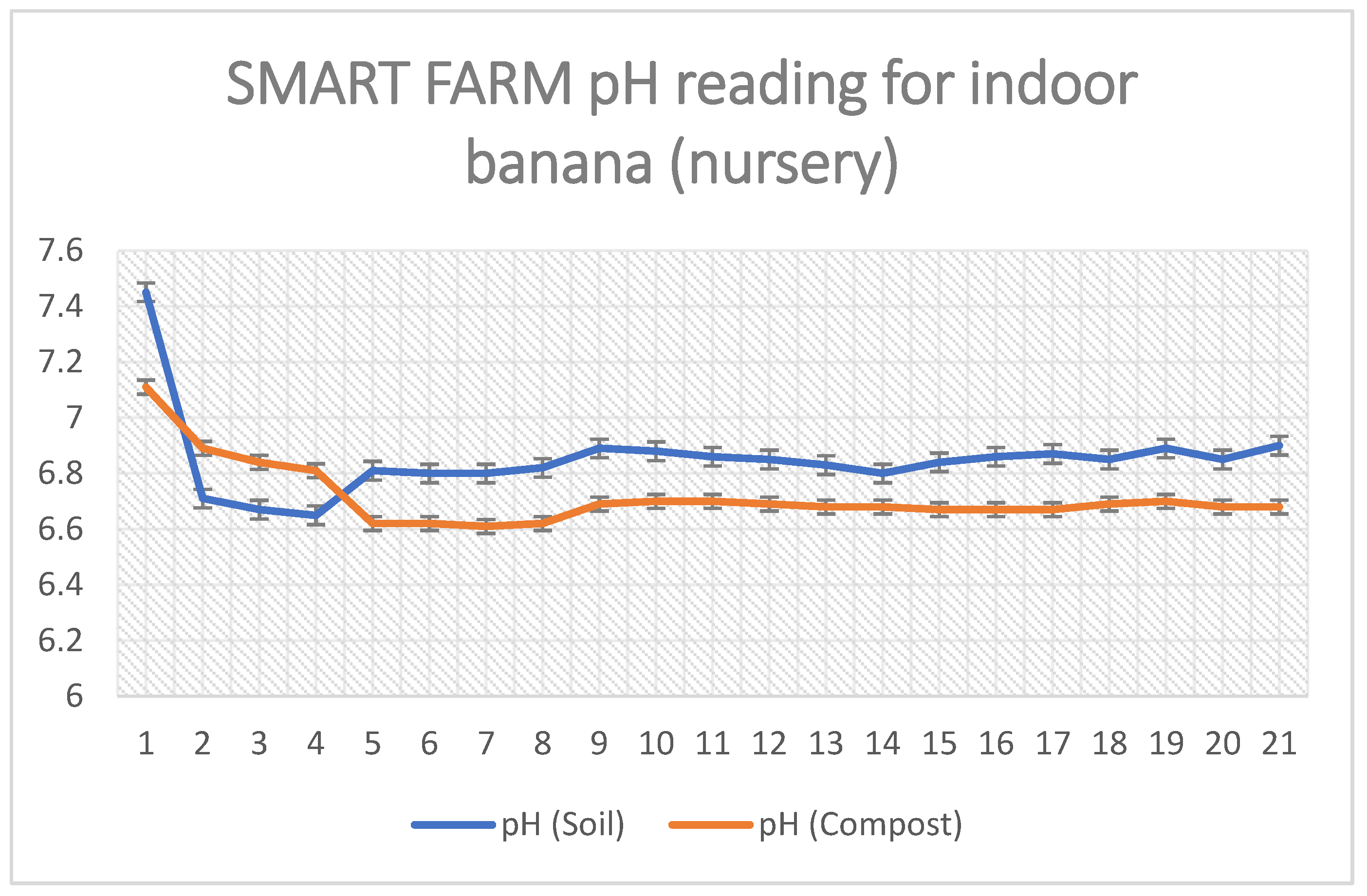
3.6. The SMART FARM pH Reading Based on the JDL Algorithms and the CNN

With the onboard pH sensor for the soil, we could measure the pH levels in the nursery based on the soil and the compost. When the pH value decreases below seven, the soil becomes increasingly acidic. Any value greater than seven corresponds to a higher level of alkalinity. Each pH sensor variant operates distinctively to assess the soil’s quality. The sensor operates by comparing the electrical potential of a pH-sensitive system to the potential of a stable reference system. A sensor electrode detects and quantifies the electrical potential of the glass bulb. The ideal soil for growing bananas should possess high fertility, excellent drainage, abundant organic matter, and the ability to retain moisture. The optimal pH range is between 6.5 and 7.5, as bananas have a minor preference for acidity, which is confirmed in Figure 15.

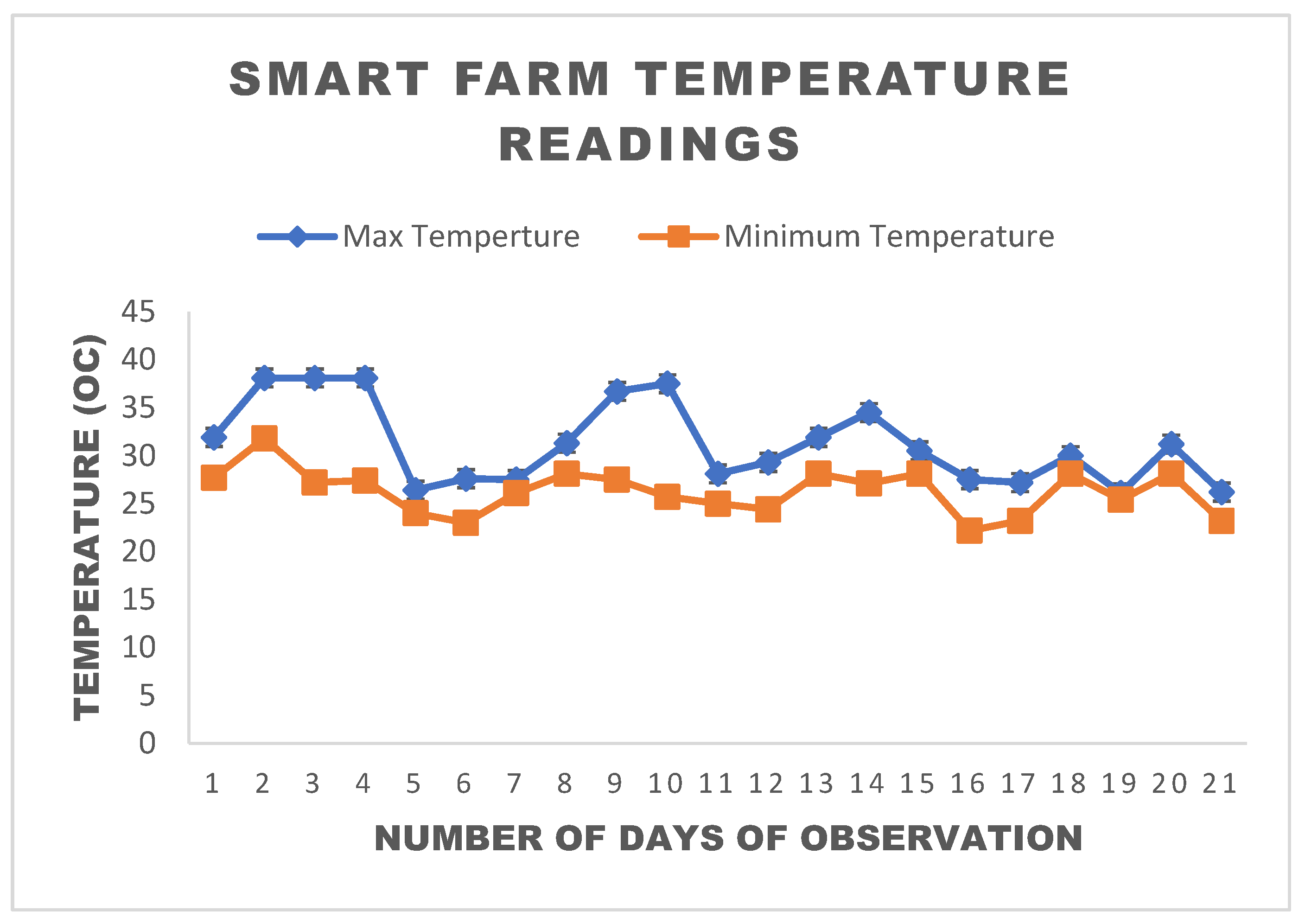
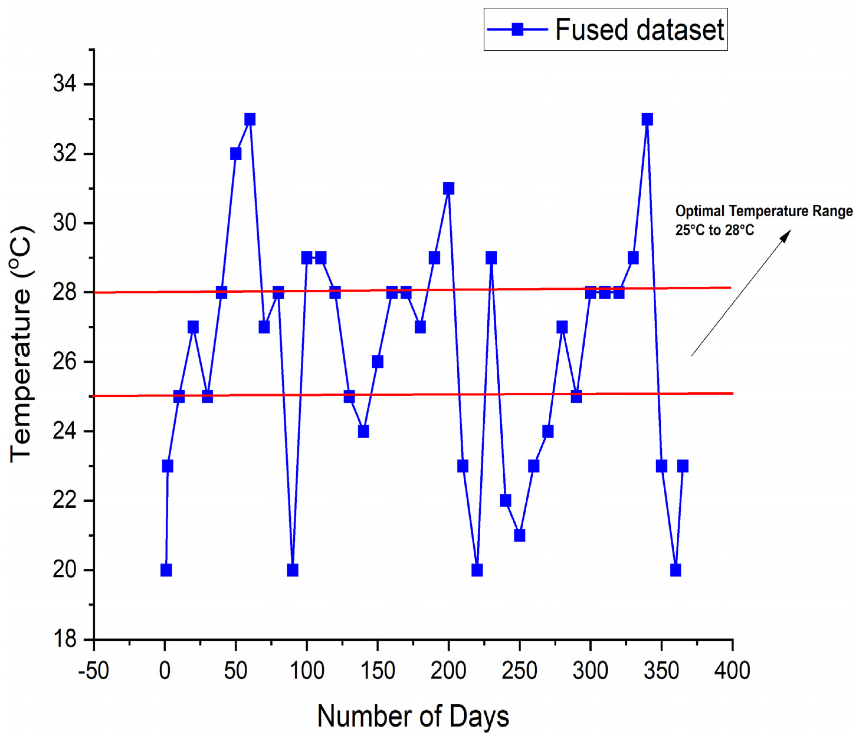
3.7. Temperature and Humidity Based on JDL Algorithms and the CNN

The banana plant is highly thermophilic, and exposure to low temperatures can harm its well-being. As shown in Figure 16, the indoor maximum temperature is 38.1 °C and the minimum is 21 °C, which are ideal temperatures for banana cultivation and align with the literature concerning banana temperature requirements. Elevated temperatures, even for brief durations, impact the growth of crops, particularly temperate varieties such as wheat. Elevated air temperatures inhibit shoot growth, thereby diminishing root development. An elevated soil temperature is dangerous as it inflicts significant harm to the roots, leading to a considerable decline in shoot growth. Therefore, high temperature stress reduces nutrition uptake and assimilation. In bananas, both soil and air temperature affect nutrient uptake.

Elevated temperatures frequently correspond to reduced humidity levels in the greenhouse where the banana was cultivated. Therefore, SMART FARM was installed to monitor the temperature and humidity fluctuations within the indoor environment, as seen in Figure 17. The water requirement estimation approach was used to assess the transpiration of bananas within the greenhouse environment. Transpiration is governed by a model established by

$$Tr=\delta r_a\left(R_{net}-F_s\right)+{\displaystyle \frac{p{C}_{p}LAI{D}_{sat}}{\delta r_a+2\gamma (r_i+r_a)}}$$

(13)

where Tr = transpiration flow (W/m²), Dsat = saturation deficit (mbar), Fs = thermal flux in soil (W/m²), ‘γ’ = psychometric constant (mb/°C), R = net radiation (W/m²), Cp = air-specific heat at constant pressure (J/Kg°C), ra = aerodynamic resistance (s/cm), ‘i’ = interior, and LAI = Leaf Area Index.

Equation (13) is based on estimating two parameters: the Leaf Area Index (LAI) and the resistance ‘r_i’ of the stomata. The LAI is then determined based on the relationship between the surface of the sheet and the dimension characteristic, and the stomata resistance is also calculated based on the radiation, with ‘r_min’ being the minimum resistance expressed exponentially.

$$S=0.64\left(L\times l\right)+1416.82$$

(14)

$$r_s=r_{min}[1+exp0.0033(R_g-516.505{)}^{-1}]$$

(15)

To validate the CNN model on the banana leaf development, water stress, and the amount of water needed per day in the greenhouse, we estimated the water need from

$$WN={\displaystyle \frac{K_c\times T_r.A_T}{L_v}}$$

(16)

where ‘WN’ is water need, L_v is latent heat of water vaporisation (J/Kg), AT is soil surface of the greenhouse (m²), L is most excellent length of leaf (m), l is greatest width of leaf (m), Rg is global solar radiation (W/m²), ri is internal resistance of the leaf, RH is relative air humidity (%), T is temperature, °C, Tr is transpiration flow (W/m²), u is wind speed (m/s), ‘e’ is exterior, ‘f’is leaf, and ‘s’ is soil. The cultural coefficient, $K_c$, represents the ratio of crop evapotranspiration to potential evapotranspiration.

$K_c$ is contingent upon the crop’s attributes, planting dates, pace of development, length of vegetative cycle, climatic conditions, particularly during the initial growth phase, and frequency of irrigation.

Tuzet and Perrier [20] assert that $K_c$primarily fluctuates based on the unique attributes of the crop, with minimal influence from climatic factors. This facilitates the transfer of standard $K_c$ values across different climatic zones [32].

For our model, we considered the mid-season time, when the banana plant was at its peak of development. The estimated ‘K_C’ was then achieved by

$$K_c=K_c\left(tab\right)+[0.04\left(u-2\right)-0.004({RH}_{min}-45\left)\right]({\displaystyle \frac{h}{3}}{)}^{0.3}$$

(17)

where ‘K_c(tab)’ is the value of data given by [32], ‘u’ represents the average wind speed recorded, and ‘h’ represents the plant’s average height.

Based on the sensor readings, banana plants needed 10–20 litres of water daily during their growing season. However, there were fluctuations due to the hot climate, soil composition, and growth stage.

It is stated in the literature that in arid and high-temperature environments, banana plants may require as much as 40 litres of water daily; this falls in line with this study, where based on Figure 18, water demand on December 18 went as high as 36 litres per day. The plant’s water needs, depicted in Figure 18, were derived from soil moisture sensors embedded in the soil adjacent to the roots, quantifying water content and signalling when the soil is desiccated and requires irrigation. The signals and data are subsequently analysed by a microcontroller and the SMART FARM monitoring system to ascertain the plant’s current water requirements, activating the irrigation system accordingly.

The transpiration ratio of the plants during the hot climate period was also noted to range from 100 to 600, indicating that the banana plants transpired 100 to 600 kg of water for each kilogram of dry matter produced (see Figure 19).

According to the literature, the Leaf Area Index (LAI) for a well-managed banana plantation can range from 0 at planting to 5 at maturity. Looking at Figure 20, with the LAI ranging from 3.3 in June to 4.89 in December, our proposed system for monitoring bananas in a greenhouse will give the farmer accurate information about the bananas in and around the greenhouse.

The different datasets indicate temperature variations (Figure 21) that will impact the growth and development of bananas in the greenhouse. This occurs because photosynthesis, transpiration, and respiration intensify when temperature rises (up to a certain threshold). Temperature, in conjunction with day length, influences the transition from vegetative (leafy) to reproductive (flowering) growth [33].

The optimal temperature range for bananas is between 20 °C and 30 °C, with an ideal range of 25 °C to 28 °C. This aligns with the existing literature [33], as shown by the study’s integrated datasets (see Figure 22). It should be noted that high temperature (HT) stress constitutes a significant environmental challenge that restricts banana growth and metabolism, as banana growth and development encompass various temperature-sensitive biochemical reactions.

4. Discussion

The optimal soil for cultivating bananas must have high fertility, superior drainage, ample organic matter, and moisture retention capabilities. The preferred pH range is between 6.5 and 7.5, indicating a slight inclination for acidity, as illustrated in Figure 15. The banana plant is extremely heat-loving, and exposure to low temperatures can adversely affect its health. As shown in Figure 17, the indoor maximum temperature was 38.1 °C and the minimum was 21 °C, which are optimal temperatures for banana production. These data align with the literature regarding the temperature requirements for bananas.

In a moderately hot climate, with an average wind speed of approximately 2 m/s, we adopted an average value of Kc equal to 1.15. We selected December, which is representative of hotter times, to estimate the water requirements for our greenhouse. The computations were conducted from December 10 to December 28. The diurnal interval was analysed from 08:00 to 18:00, and the peak daily transpiration value was assessed for this timeframe. The results acquired are illustrated in Figure 18, where the ‘WN’ values, as indicated by Equation (17), range from 25 to 50 m³/(ha·J). These discrepancies are attributable to the fluctuations in the maximum daily transpiration as indicated by Equation (13) and illustrated in Figure 19. Again, the variations in LAI are depicted in Figure 20, where the average ‘WN’ value is approximately 40 m per acre per day.

This result closely aligns with the literature, which ranges from 40 to 50 m³ per acre per day. Ref [34] reports that farms employing the Circo jet in conjunction with misting practises exhibit application rates ranging from 12 to 16,000 m³/ha per day, precisely 33 to 44 m³. Sensor data indicated that banana plants need 10–20 litres of water daily during their growing season, with variations attributed to the hot climate, soil composition, and growth stage. The literature indicates that banana plants may require up to 40 litres of water daily in arid, high-temperature settings. This aligns with the study illustrated in Figure 18, where water consumption on December 18 reached 36 litres daily. The transpiration ratio of the plants throughout the hot climate period ranged from 100 to 600, signifying that the banana plants transpired 100 to 600 kg of water for every kilogram of dry matter generated (see Figure 19). The research indicates that the Leaf Area Index (LAI) for a well-managed banana plantation can vary from 0 at planting to 5 at maturity. Figure 20 illustrates that the Leaf Area Index (LAI) ranges from 3.3 in June to 4.89 in December. This indicates that our suggested system for monitoring bananas in a greenhouse will provide the farmer with precise information regarding the bananas within and surrounding the greenhouse.

We employed optical instruments to measure the Leaf Area Index (LAI) by measuring contact frequency and gap fraction. The ideal Leaf Area Index for achieving yield potential was noted to be between 3.6 and 4.5 [35]. The daily humidity and temperature readings in Figure 17 also show that the ideal relative humidity level for bananas is approximately 80%, typically ranging from 65% to 75% at night and around 80% during the day. Fluctuations in humidity can impede the plant’s physiological functions, resulting in reduced growth rate and diminished crop quality [36]. The fused dataset shows that the optimal temperature range for bananas is between 20 °C and 30 °C, with an ideal range of 25 °C to 28 °C. This is consistent with the current literature [33], as evidenced by the study’s integrated datasets (Figure 22). The JDL–Mivar crop model utilises quantitative parameters to forecast plant growth and development under varying environmental conditions.

The model identified the mathematical correlations between bananas and their surroundings (weather and soil). The model again utilised mathematical relationships to replicate various elements of crop performance and imitate the growth and development of a crop. The model’s data integration technology compiles agricultural facts to create a digital model designed for detailed simulations of crop and environmental interactions [37]. Algorithms are precise instructions for calculating and manipulating the data. Advanced algorithms can utilise conditionals to direct the execution of code along several paths (known as automated decision-making) and derive accurate conclusions (known as automated reasoning) [38], thus attaining automation.

5. Conclusions

In this study, a banana environment monitoring system was developed based on the JDL fusion model. Sensors were installed in the greenhouse, and data were obtained from the WSN. This was performed to evaluate the actual optimum conditions needed for cultivating bananas in a closed environment like the greenhouse. The JDL model with Mivar was introduced because the study applied the model to indoor banana cultivation. The study employed Python programming and CNN for the monitoring since forecasting soil moisture is crucial for ascertaining optimal irrigation timing and water application volume, hence mitigating issues related to over- and under-watering.

The progression of primary average climatic parameters, including the interior and outdoor temperature, humidity, pH, and transpiration, was observed. After the study, it was determined that the optimal indoor maximum temperature for banana production was 38.1 °C, while the minimum was 21 °C. The water need (WN) values ranged from 25 to 50 m³/(ha·J), with notable differences and oscillations in the maximum daily transpiration. The WSN moisture sensor data revealed that banana plants require 10–20 litres of water daily during their growing season. The transpiration ratio of the plants throughout the hot climate period varied from 100 to 600, indicating that the banana plants transpired 100 to 600 kg of water for each kilogram of dry matter produced. The Leaf Area Index (LAI) fluctuated from 3.3 in June to 4.89 in December, demonstrating that our proposed technique for monitoring bananas in a greenhouse will furnish the farmer with accurate information on the bananas within the greenhouse.

The optimal Leaf Area Index for maximising yield potential is between 3.6 and 4.5, with a relative humidity level for bananas of approximately 80%, generally fluctuating from 65% to 75% at night and about 80% during the day. The model employed mathematical relationships to simulate several aspects of agricultural performance and duplicate the growth and development of a crop. The model’s data integration technology aggregates agricultural data to construct a digital model intended for comprehensive simulations of crop and environmental interactions. Algorithms function as explicit directives for calculating and managing data to provide an optimal growth environment for bananas. The assessment of water requirements and the implementation of efficient irrigation practises are essential for the advancement of greenhouse banana agriculture. We have introduced the JDL model to estimate the optimum growth requirements of a greenhouse banana crop under actual growth conditions. The results achieved closely align with those suggested in the literature. The subsequent phase seeks to enhance the model and accurately ascertain the cultural coefficient of the location.

References

1. Bolfe, É.L.; Jorge, L.A.d.C.; Sanches, I.D.A.; Luchiari Júnior, A.; da Costa, C.C.; Victoria, D.d.C.; Inamasu, R.Y.; Grego, C.R.; Ferreira, V.R.; Ramirez, A.R. Precision and digital agriculture: Adoption of technologies and perception of Brazilian farmers. Agriculture 2020, 10, 653. [Google Scholar] [CrossRef]
2. Escotet, M.Á. The optimistic future of Artificial Intelligence in higher education. Prospects 2023, 1–10. [Google Scholar] [CrossRef]
3. Miine, L.K.; Akorsu, A.D.; Boampong, O.; Bukari, S. Digital agriculture and decent working conditions of smallholder farmers and farmworkers in Ghana. Discov. Food 2024, 4, 173. [Google Scholar] [CrossRef]
4. Lajoie-O’Malley, A.; Bronson, K.; van der Burg, S.; Klerkx, L. The future (s) of digital agriculture and sustainable food systems: An analysis of high-level policy documents. Ecosyst. Serv. 2020, 45, 101183. [Google Scholar] [CrossRef]
5. Droste, N.; May, W.; Clough, Y.; Börjesson, G.; Brady, M.; Hedlund, K. Soil carbon insures arable crop production against increasing adverse weather due to climate change. Environ. Res. Lett. 2020, 15, 124034. [Google Scholar] [CrossRef]
6. Corejova, T.; Chinoracky, R. Assessing the Potential for Digital Transformation. Sustainability 2021, 13, 11040. [Google Scholar] [CrossRef]
7. Yamini, B.; Pradeep, G.; Kalaiyarasi, D.; Jayaprakash, M.; Janani, G.; Uthayakumar, G.S. Theoretical study and analysis of advanced wireless sensor network techniques in Internet of Things (IoT). Meas. Sens. 2024, 33, 101098. [Google Scholar] [CrossRef]
8. Naeem, M.; Jamal, T.; Diaz-Martinez, J.; Butt, S.A.; Montesano, N.; Tariq, M.I.; De-la-Hoz-Franco, E.; De-La-Hoz-Valdiris, E. Trends and future perspective challenges in big data. In The Advances in Intelligent Data Analysis and Applications, Proceeding of the Sixth Euro-China Conference on Intelligent Data Analysis and Applications, Arad, Romania, 15–18 October 2019; Springer: Singapore, 2022; pp. 309–325. [Google Scholar]
9. Steinberg, A.N.; Bowman, C.L.; White, F.E.; Blasch, E.P.; Llinas, J. Evolution of the JDL model. Perspect. Inf. Fusion 2023, 6, 36–40. [Google Scholar]
10. Munkhdalai, L.; Munkhdalai, T.; Pham, V.-H.; Li, M.; Ryu, K.H.; Theera-Umpon, N. Recurrent neural network-augmented locally adaptive interpretable regression for multivariate time-series forecasting. IEEE Access 2022, 10, 11871–11885. [Google Scholar] [CrossRef]
11. Wang, M.; Song, G.; Yu, Y.; Zhang, B. The current research status of AI-based network security situational awareness. Electronics 2023, 12, 2309. [Google Scholar] [CrossRef]
12. Teixeira, A.V.; Rezende, D.A. A multidimensional information management framework for strategic digital cities: A comparative analysis of Canada and Brazil. Glob. J. Flex. Syst. Manag. 2023, 24, 107–121. [Google Scholar] [CrossRef]
13. Huang, J.; Naini, S.S.; Miller, R.; Rizzo, D.; Sebeck, K.; Shurin, S.; Wagner, J. A hybrid electric vehicle motor cooling system—Design, model, and control. IEEE Trans. Veh. Technol. 2019, 68, 4467–4478. [Google Scholar] [CrossRef]
14. Peykova, A.; Petrova-Antonova, D.; Karamitov, K. Data Processing and Enrichment of LiDAR-Derived Traffic Data. ISPRS Ann. Photogramm. Remote Sens. Spat. Inf. Sci. 2024, 10, 263. [Google Scholar] [CrossRef]
15. Vignesh, T.; Gowrishankar, S.; Jishnu, M.; Prithvi, J.K.; Joseph, P.L.; Devi, P.K.D. Influence of telepresence robot using arduino UNO R3 based 20A robot control board. In Proceedings of the 1st International Conference on Frontier of Digital Technology Towards a Sustainable Society, organized by the University, Malaysia, Malaysia, 22 May 2023. [Google Scholar]
16. Aboudzadeh, M.A.; Hamzehlou, S. Supramolecular Ionic Networks: Properties. In Supramolecular Assemblies Based on Electrostatic Interactions; Springer: Berlin/Heidelberg, Germany, 2022; pp. 29–54. [Google Scholar]
17. Carcaterra, A. Minimum-variance-response and irreversible energy confinement. In The IUTAM Symposium on the Vibration Analysis of Structures with Uncertainties: Proceedings of the IUTAM Symposium on the Vibration Analysis of Structures with Uncertainties Held in St. Petersburg, Russia, July 5–9, 2009; Springer: Dordrecht, The Netherlands, 2011; pp. 215–228. [Google Scholar]
18. Mazumder, S. Use of Integrated Crop Management (ICM) Practices by the Farmers of Pirojpur District. Master’s Thesis, Department of Agricultural Extension and Information System, Sher-e-Bangla Agricultural University, Dhaka, Bangladesh, 2018. [Google Scholar]
19. Zhang, X.; He, K.; Sima, Q.; Bao, Y. Error-feedback three-phase optimization to configurable convolutional echo state network for time series forecasting. Appl. Soft Comput. 2024, 161, 111715. [Google Scholar] [CrossRef]
20. Badamasi, Y.A. The working principle of an Arduino. In Proceedings of the 2014 11th International Conference on Electronics, Computer and Computation (ICECCO), Abuja, Nigeria, 29 September–October 2014; pp. 1–4. [Google Scholar]
21. Prema, R.; Jahnavi, V.; Reddy, S.V. Smart Surveillance System using Python and OpenCV. Int. J. Sci. Res. Eng. Manag. 2023. [Google Scholar]
22. Richards, J.A.; Richards, J.A. Remote Sensing Digital Image Analysis; Springer: Berlin/Heidelberg, Germany, 2022; Volume 5. [Google Scholar]
23. Sabado-Burlat, C.; Ignacio, M.T.T.; Guihawan, J. Inventory of high value crops using lidar data and gis in lanao del norte philippines. ASEAN Eng. J. 2022, 12, 183–187. [Google Scholar] [CrossRef]
24. Dibbo, S.V.; Cheung, W.; Vhaduri, S. On-Phone CNN Model-Based Implicit Authentication to Secure IoT Wearables. In The Fifth International Conference on Safety and Security with IoT; Springer: Cham, Switzerland, 2023. [Google Scholar]
25. Agbozo, E.; Balungu, D.M. Liver Disease Classification—An XAI Approach to Biomedical AI. Informatica 2024, 48, 03505596. [Google Scholar] [CrossRef]
26. Zheng, K.; Qian, Y.; Yuan, Z.; Peng, F. Centrosymmetric constrained Convolutional Neural Networks. Int. J. Mach. Learn. Cybern. 2024, 15, 2749–2760. [Google Scholar] [CrossRef]
27. Patrignani, A.; Ochsner, T.E. Canopeo: A powerful new tool for measuring fractional green canopy cover. Agron. J. 2015, 107, 2312–2320. [Google Scholar] [CrossRef]
28. Wilson, J.B. Cover plus: Ways of measuring plant canopies and the terms used for them. J. Veg. Sci. 2011, 22, 197–206. [Google Scholar] [CrossRef]
29. Ashapure, A.; Jung, J.; Chang, A.; Oh, S.; Maeda, M.; Landivar, J. A comparative study of RGB and multispectral sensor-based cotton canopy cover modelling using multi-temporal UAS data. Remote Sens. 2019, 11, 2757. [Google Scholar] [CrossRef]
30. Kaewchote, J.; Janyong, S.; Limprasert, W. Image recognition method using Local Binary Pattern and the Random Forest classifier to count post larvae shrimp. Agric. Nat. Resour. 2018, 52, 371–376. [Google Scholar] [CrossRef]
31. Dale, J.; Burnside, N.G.; Hill-Butler, C.; Berg, M.J.; Strong, C.J.; Burgess, H.M. The use of unmanned aerial vehicles to determine differences in vegetation cover: A tool for monitoring coastal wetland restoration schemes. Remote Sens. 2020, 12, 4022. [Google Scholar] [CrossRef]
32. Pereira, L.; Paredes, P.; Jovanovic, N. Soil water balance models for determining crop water and irrigation requirements and irrigation scheduling focusing on the FAO56 method and the dual Kc approach. Agric. Water Manag. 2020, 241, 106357. [Google Scholar] [CrossRef]
33. Abdalla, Z.F.; El-Ramady, H. Applications and Challenges of Smart Farming for Developing Sustainable Agriculture. Environ. Biodivers. Soil Secur. 2022, 6, 81–90. [Google Scholar] [CrossRef]
34. Fandiño, M.; Cancela, J.; Rey, B.; Martínez, E.; Rosa, R.; Pereira, L. Using the dual-Kc approach to model evapotranspiration of Albariño vineyards (Vitis vinifera L. cv. Albariño) with consideration of active ground cover. Agric. Water Manag. 2012, 112, 75–87. [Google Scholar] [CrossRef]
35. Israeli, Y.; Lahav, E. Injuries to banana caused by adverse climate and extreme weather. In Handbook of Diseases of Banana, Abacá and Enset; CAB International: Wallingford, UK, 2019; pp. 487–526. [Google Scholar]
36. Ravi, I.; Vaganan, M.M. Abiotic stress tolerance in banana. In Abiotic Stress Physiology of Horticultural Crops; Springer: Berlin/Heidelberg, Germany, 2016; pp. 207–222. [Google Scholar]
37. Botín-Sanabria, D.M.; Mihaita, A.-S.; Peimbert-García, R.E.; Ramírez-Moreno, M.A.; Ramírez-Mendoza, R.A.; Lozoya-Santos, J.d.J. Digital twin technology challenges and applications: A comprehensive review. Remote Sens. 2022, 14, 1335. [Google Scholar] [CrossRef]
38. Varlamis, I.; Michail, D.; Glykou, F.; Tsantilas, P. A survey on the use of graph convolutional networks for combating fake news. Future Internet 2022, 14, 70. [Google Scholar] [CrossRef]
Figure 1. Global state estimation problem.
Water 17 00325 g001
Figure 2. Control and data receiver connection build-up.
Water 17 00325 g002
Figure 3. The concept of interaction between SMART FARM and its external environment.
Water 17 00325 g003
Figure 4. Finished data engine control adopted from [15].
Water 17 00325 g004
Figure 5. Finished app interface for phone and computer communication.
Water 17 00325 g005
Figure 6. SMART FARM app’s communication outline (from crop producers to buyers).
Water 17 00325 g006
Figure 7. Algorithm flowchart for the JDL–Mivar model employed for SMART FARM.
Water 17 00325 g007
Figure 8. Circuit diagram for Arduino adopted in this study [20].
Water 17 00325 g008
Figure 9. SMART FARM model programming rule with the JDL–Mivar model.
Water 17 00325 g009
Figure 10. Classification of the banana water stress with CNN model.
Water 17 00325 g010
Figure 11. Convolutional networks to forecast planted bananas.
Water 17 00325 g011
Figure 12. Well-established banana in the greenhouse environment under the SMART FARM model.
Water 17 00325 g012
Figure 13. The banana canopy cover trends.
Water 17 00325 g013
Figure 14. The training and testing/validation accuracy of the CNN model for the original image dataset at different sampling dates.
Water 17 00325 g014
Figure 15. SMART FARM app pH readings.
Water 17 00325 g015
Figure 16. SMART FARM temperature readings.
Water 17 00325 g016
Figure 17. The daily temperature and relative humidity of the greenhouse.
Water 17 00325 g017
Figure 18. Daily variations in water requirements for greenhouse bananas in hot, dry climate (December).
Water 17 00325 g018
Figure 19. Daily variations in maximum greenhouse transpiration values for bananas in December.
Water 17 00325 g019
Figure 20. Time course of the greenhouse banana crop’s LAI.
Water 17 00325 g020
Figure 21. Individual temperature dataset.
Water 17 00325 g021
Figure 22. Fused temperature.
Water 17 00325 g022