Review

The Theoretical Basis of qPCR and ddPCR Copy Number Estimates: A Critical Review and Exposition

1
Robert B. Annis Water Resources Institute, 740 West Shoreline Dr., Muskegon, MI 49441, USA
2
Department of Statistics, Grand Valley State University, Mackinac Hall, 1 South Campus Drive, Allendale, MI 49401, USA
3
Department of Civil, Environmental, and Geodetic Engineering, Ohio State University, 2070 Neil Avenue, Columbus, OH 43210, USA
4
Department of Chemistry, Oakland University, 146 Library Drive, Rochester, MI 48309, USA
*
Author to whom correspondence should be addressed.
Current address: Geosyntec Consultants, Inc., 500 West Wilson Bridge Road, Suite 250, Worthington, OH 43085, USA.
Water 2025, 17(3), 381; https://doi.org/10.3390/w17030381
Submission received: 21 December 2024 / Revised: 16 January 2025 / Accepted: 28 January 2025 / Published: 30 January 2025

Abstract

:
The polymerase chain reaction (PCR) is a molecular biology tool with diverse applications in the aquatic sciences. Classical PCR is a nonquantitative method that can be used to detect target DNA sequences that are characteristic of particular microbial taxa but cannot determine their concentrations in water samples. Various quantitative forms of PCR have been developed to remove this limitation. Of these, the two that currently are used most widely are real-time quantitative PCR (qPCR) and droplet digital PCR (ddPCR). Several outlines of the mathematical and statistical basis of these methods for estimating target sequence concentrations are available in the literature, but we are aware of no thorough and rigorous derivation of the theoretical underpinnings of either. The purpose of this review is to provide such derivations, and to identify and compare the main strengths and weaknesses of the two methods. We find that both estimation methods are sound, provided careful attention is paid to specific details that differ between the two. With qPCR, it is especially important to reduce any significant PCR inhibition by sample constituents and to properly fit the standard curve to heteroskedastic calibration data. With ddPCR, it is important to ensure that the value of the mean droplet volume used in calculating concentrations is correct for the particular combination of droplet generator and master mix used. The advantages of qPCR include lower instrument and per-sample costs, a shorter turnaround time for obtaining results, a higher upper limit of quantification, and a wider dynamic range. The advantages of ddPCR include freedom from dependence on a standard curve, an inherently lower sensitivity to PCR inhibitors, a lower limit of quantification, a simpler theoretical basis, and simpler data analysis. We suggest qPCR often will be preferable in laboratory studies where investigators have significant control over the range of target sequence concentrations in samples, concentrations are sufficiently high so proper calibration does not require standards with concentrations low enough to exhibit exaggerated variability in the threshold cycle, and no significant inhibition is present, or more generally, in studies where funding levels do not permit the higher cost of instrumentation and supplies required by ddPCR or where the shorter turnaround time for qPCR is essential. If sufficient funds are available, ddPCR often will be preferable when the ability to quantify low concentrations is important, especially if inhibitors are likely to be present at concentrations that are problematic for qPCR.

1. Introduction

The polymerase chain reaction (PCR) is a fundamental tool of molecular biology that has found widespread application in the biological and environmental sciences. An early form of PCR was developed in the late 1960s by Kjell Kleppe, who called it “repair replication” [1]. The modern form was conceived in 1983 by Kary Mullis, who subsequently developed a practical and efficient method that he published in a series of papers with various collaborators [2,3,4]. Mullis shared the 1993 Nobel Prize in Chemistry for this work.
PCR is, essentially, a molecular copy machine that can rapidly generate billions of copies of a short DNA sequence. In environmental studies, it can be used in conjunction with gel electrophoresis and a fluorescent DNA stain to provide a visual presence/absence assay for target DNA sequences from specific groups or organisms (e.g., [5,6]). Standard PCR, however, provides no quantitative information about the concentrations of the target sequences in a sample. For example, while standard PCR can detect target sequences characteristic of enterococci fecal indicator bacteria in recreational beach water samples, it cannot determine their concentration and, therefore, cannot be used to either establish or assess compliance with a numerical criterion for protecting human health, such as a Beach Action Value [7]. Various elaborations of PCR have been developed since the 1980s to address this important limitation. Of these quantitative PCR methods, the two that are most widely used at the present time are real-time quantitative PCR (qPCR) and droplet digital PCR (ddPCR).
Real-time quantitative PCR was first developed by Higuchi and others in the early 1990s [8]. The key idea underlying its ability to determine the concentration of a target sequence in a sample is to introduce a unique fluorescent label or dye whose level of fluorescence is tightly linked to amplification of the target DNA sequence by PCR, so that fluorescence of a sample increases as the number of amplicons increases. Unlike the concentration of the amplicons themselves, fluorescence can easily be monitored in real-time and, with additional information from a standard curve, the temporal pattern of increase can be used to back-calculate the initial number of copies in the sample. The dependence of this approach on monitoring the polymerase chain reaction in real-time is the key feature that distinguishes it from endpoint types of quantitative PCR, such as chamber-based digital PCR (cdPCR) and ddPCR [9]. The acronym “qPCR” is now generally recognized to denote specifically real-time quantitative PCR.
The original forms of digital PCR also were developed in the 1990s [10,11]. These methods were based on the idea of diluting extracted DNA containing the target sequence to such a degree that most wells in a multi-well PCR plate will contain either no copies of the sequence or only a small number. Sample wells containing the extracted DNA and an assay mix that included a fluorescent dye were processed simultaneously as replicate endpoint PCR reactors. The concentration of the target DNA sequence was estimated from the proportion of wells that failed to fluoresce above a user-specified threshold level (hence, contained no copies of the target sequence), using a probability argument based on the Poisson distribution. The important advantages over qPCR were a reduced sensitivity to PCR inhibition and the fact that no standard curve was required.
The modern droplet-based form of digital PCR was developed during the late 1990s and early 2000s and employs microfluidics technology [12,13,14,15]. With this method, extracted DNA containing the target sequence (along with an assay mix that includes a fluorescent dye) is partitioned into thousands of microscopic droplets per sample well that are so small that most will contain either no copies of the target sequence or only a very small number. The temperature cycling that drives PCR amplification is then performed simultaneously on all the droplets, which serve as replicate endpoint PCR reactors. Each droplet fluoresces above a user-specified threshold level at the reaction endpoint if and only if at least one copy of the target sequence was included in the droplet when formed (and was then amplified). As in the dilution form of digital PCR, the proportion of droplets that fail to fluoresce above the threshold, as determined by a droplet reader, is used to estimate the concentration of the target sequence, and no standard curve is required. Thus, ddPCR achieves the same outcome as earlier forms of digital PCR but with far less dilution of the sample and a vastly larger number of replicate reactions. ddPCR currently is more expensive than qPCR and has a somewhat longer sample processing time, but it also has important advantages in environmental applications (notably, no dependence on a standard curve and reduced sensitivity to interference) and, therefore, is increasingly being used in place of qPCR.
Like standard PCR, qPCR and ddPCR were originally developed for applications in molecular biology. However, both methods are now reasonably common in environmental studies of aquatic systems, including natural waterbodies as well as wastewater. Examples of applications include water quality monitoring [16,17,18], microbial source tracking [19,20,21,22,23,24,25,26,27], species detection using environmental DNA [28,29,30], and wastewater-based epidemiology [31,32,33,34,35].
The purpose of this paper is to systematically develop what we believe to be the mathematical and statistical foundations of qPCR and ddPCR in sufficient detail to identify key underlying assumptions that may affect the accuracy and precision of concentration estimates and, more broadly, to answer two fundamental questions to the reader’s and our own satisfaction:
  • How does qPCR make it possible to estimate the initial copy number in an environmental sample by monitoring, in real-time, the increasing fluorescence during successive PCR cycles, using additional information derived from a standard curve?
  • How does ddPCR make it possible to estimate the initial copy number in a sample by determining the proportion of droplets that do not fluoresce above background at the reaction endpoint, without requiring a standard curve?
Some of the details of our presentation will no doubt reflect the specific analytical instruments we normally use for qPCR and ddPCR analysis, which are the Applied Biosystems® StepOnePlusTM real-time qPCR system and the Bio-Rad® QX200TM ddPCR system. The basic principles, however, appear to be general.
Software accompanying laboratory instruments that perform qPCR and ddPCR carry out all the necessary calculations and report the estimated copy numbers, but we are philosophically opposed to trusting proprietary software to perform calculations that are not fully documented and whose software implementation cannot be checked. Some of the necessary information about these calculations is available in the literature (e.g., [9,36,37,38]) and on instrument manufacturer and vendor websites (e.g., [39,40]), but all the accounts we are aware of are incomplete, and some of the information is overly simplified and not entirely correct. We, therefore, set out to determine for ourselves whether rigorous quantitative theories can be developed for qPCR and ddPCR that justify placing trust in the numbers that commercial software produces. As will be shown, the answer is a qualified “yes” for both qPCR and ddPCR.
The paper is organized as follows. We address qPCR first, then ddPCR. For each method, we begin with an overview, then develop the underlying mathematical and statistical theory, and finally, we present an example where we apply the theory to some of our own data. We conclude with a brief discussion comparing what we see as the strengths and weaknesses of the two methods when used to quantify DNA target sequences in environmental samples, especially in studies of aquatic systems.

2. Real-Time Quantitative PCR

2.1. A Brief Overview of qPCR

Numerous protocols for the qPCR analysis of environmental samples are available in the literature and on instrument manufacturer and vendor websites (an example of a qPCR workflow that has been widely used in the state of Michigan for monitoring E. coli contamination at recreational beaches is presented in Appendix A). Regardless of which protocol one uses, the first step in this process is sample preparation. In studies quantifying the abundances of aquatic microorganisms such as bacteria or unicellular algae, cells of the focal taxonomic group (as well as others) are collected from water samples, usually by filtration, and then, are physically or chemically lysed, releasing the genetic material they contain for subsequent exposure to the reagents employed in qPCR analysis.
Crude extracts from physical lysis procedures such as bead milling, consisting of the supernatants of these samples after centrifugation, are often directly analyzed with qPCR. However, this procedure is not very effective at removing common PCR inhibitors such as tannins, chlorophyll, and humic/fulvic acids that are collected with the cells, and it is not applicable with most chemical lysis procedures. Therefore, sample preparation processes will often include a DNA purification procedure to remove contaminants and, if necessary, concentrate the recovered genetic material.
A variety of procedures can be used to purify and concentrate extracted samples. The most common types involve the passage of the crude lysates through silica membranes, where a salt gradient binds all nucleic acids in the sample to the membrane [31,41]. After the membrane is washed to remove inhibitors and other contaminants, the genetic material is eluted and is ready for amplification.
Like standard (nonquantitative) PCR, qPCR creates a large number of copies of (i.e., amplifies) a target DNA sequence in a prepared sample if that sequence is present. Unlike standard PCR, however, it also quantifies the number of copies of the target sequence that were present before amplification. Quantification is achieved by combining the prepared sample with an assay mix (which contains forward and reverse primers that bind to the endpoints of the target DNA sequence, a fluorescent DNA dye or probe that may or may not be specific to the target sequence, a reference dye (Section 2.3.1), deoxynucleotide triphosphates (dNTPs), DNA polymerase, salts, and a buffer), and then, measuring, in real-time, the increasing intensity of fluorescence that occurs during a series of consecutive amplification cycles. Two alternative types of fluorescent dye can be used, with the most common representatives being TaqMan® probes and the SYBR® Green DNA stain. TaqMan probes are homologous to a segment of the DNA target sequence, contain separate fluorescent and fluorescence-quenching moieties (the reporter and quencher, respectively), and exhibit little fluorescence until the reporter is cleaved from the probe by the Taq DNA polymerase used to make copies of the target sequence, physically separating it from the quencher. By contrast, SYBR Green is a nonspecific DNA stain that binds mainly to the minor groove of any double-stranded DNA that is present [42] and fluoresces little unless bound to double-stranded DNA. To condense our exposition, we will restrict attention throughout this paper to TaqMan probes, which are more specific than SYBR Green and can be used for multiplexing.
Each PCR amplification cycle consists of three phases that are initiated and terminated by temperature changes, with the specific temperatures depending on the template DNA: (1) DNA denaturation to separate the two strands of DNA (temperature: typically 94–98 °C); (2) annealing of sequence-specific forward and reverse primers to the separate strands, and of the sequence-specific TaqMan probe to the appropriate single strand (temperature: typically 50–70 °C); and (3) extension of both primers by a thermostable DNA polymerase (temperature: typically 68–72 °C). During the extension phase, DNA polymerase cleaves the fluorescent moiety of the probe attached to the target sequence from the quencher moiety, producing a single fluorescing free reporter for each copy of the target DNA sequence that is present. As the cycles repeat, the number of copies of the target sequence increases geometrically (Section 2.2.1) while the number of fluorescing free reporters increases approximately geometrically (Section 2.2.2). The corresponding fluorescence level due to free reporters is initially much lower than the relatively constant background level and is, therefore, masked by background fluorescence (Figure 1). After several cycles (the actual number corresponds closely to the initial concentration of the target sequence), the rapidly increasing fluorescence level due to free reporters exceeds the background level and becomes measurable, with log-transformed fluorescence exhibiting an approximately linear increase as cycle number increases (Figure 1 and Figure 2). Eventually, the residual concentration of one or more PCR reagents is reduced to levels that begin to noticeably depress the rate of increase in fluorescence [43]. Fluorescence then exhibits a nonlinear decelerating pattern of increase on a logarithmic scale and approaches an asymptote that generally corresponds to the endpoint of standard PCR.
For reasons that will become clear in Section 2.2, estimates of the number or concentration of target sequence copies (TSC; we will use “TSC” as singular or plural, depending on context) in the original sample must be obtained from the linear portion of the log-fluorescence curve. Intuitively, this is the range of amplification cycles where the geometric increase in copy number, as reflected in the approximately geometric increase in fluorescence, reveals itself: The fluorescence “signal” due to amplification has increased sufficiently to separate itself from background “noise” but the depletion of PCR reactants is not yet sufficient to cause a clear deviation from geometric increase. A threshold level of fluorescence whose log-transformed value lies within this linear region is chosen, and the fractional cycle number at which fluorescence in a given sample crosses the threshold (i.e., the threshold cycle) is estimated by interpolation. The fundamental idea on which qPCR quantification rests is very simple: The smaller the number of amplification cycles required for fluorescence to cross this threshold, the more copies of the target sequence must have been present in the original sample.

2.2. Basic Equations of the qPCR Process

2.2.1. Number of Target Sequence Copies

The schematic diagram in Figure 3 illustrates the increase in the number of copies of a target DNA sequence and the corresponding increase in the number of fluorescing free reporters that occur as the number of PCR cycles increases. Each cycle consists of three main temperature-dependent steps (the specific temperatures listed here and in Figure 3 are commonly used for E. coli DNA):
  • Denaturation of DNA at 95 °C;
  • Annealing of target-specific forward and reverse primers and probes to the target sequence at 50 °C;
  • Extension of primers by DNA polymerase and concomitant cleavage of probes at 72 °C to yield free reporters that fluoresce when excited with the appropriate wavelength of light.
For convenience, we will refer to this cycle as the DAE (denaturation, annealing, and extension) cycle.
Figure 3 also shows that if every target sequence is amplified during each DAE cycle, then each TSC present at the beginning of a given cycle produces one new TSC and one new free reporter during the cycle. TSC and free reporters already present at the beginning of a cycle persist, so the total number of each at the end of the cycle is the sum of the old and new entities. In practice, some of the TSC present at the beginning of a cycle fail to produce a new copy during the cycle, so the process is not 100% efficient. We will assume, however, that each new TSC produced is accompanied by a new free reporter.
Assuming no degradation of existing TSC occurs, the number of copies present at the end of c DAE cycles is related to the number present at the end of c 1 cycles by the numerical balance law
Number of , TSC after , c cycles = Number of , TSC after , c 1 cycles + Number of new , TSC produced , during cycle c , c = 1 , 2 , 3 ,
To translate this verbal statement into mathematical symbols, let x ( c ) be a dimensionless function mapping cycle number c to the number of TSC present at the end of the cycle, and let ε ( 0 , 1 ] denote the average proportion of TSC that are amplified during any given DAE cycle. We follow EPA Draft Method C [44,45] in expressing copy numbers as numbers per reaction (which is dimensionless) instead of numbers per volume (which has dimension Length−3), with the reaction volume unspecified but assumed consistent in all equations. Then, ε represents the proportional efficiency of amplification. If amplification is fully efficient ( ε = 1 ), each TSC present at the beginning of a DAE cycle produces one new copy during the cycle. In the more realistic case where amplification is less than fully efficient ( 0 < ε < 1 ), most existing copies will produce new copies but some will not. In this case, each TSC present at the beginning of DAE cycle c will produce an average of ε new copies during the cycle, so the total number of new TSC produced during the cycle will be given by
Number of new , TSC produced , during cycle c = ε x ( c 1 ) .
Replacing the third term of the balance law in Equation (1) with this expression, and replacing the first and second terms with x ( c ) and x ( c 1 ) , we find that
x ( c ) = x ( c 1 ) + ε x ( c 1 ) = ( 1 + ε ) x ( c 1 ) = λ x ( c 1 ) , c = 1 , 2 , 3 , ,
where λ is the amplification factor defined by
λ : = 1 + ε > 1 .
Symbols and associated dimensions used in the qPCR equations here and below are summarized in Table 1.
Equation (2) is a homogeneous first-order linear difference equation with initial condition x ( 0 ) = x 0 > 0 , where initial copy number x 0 is treated as a constant. Solving this equation by backward iteration, we find that
x ( c ) = x 0 λ c , c = 0 , 1 , 2 , ,
which is geometric in cycle number c (cf. [38]). (Note: x ( c ) is a geometric sequence, because x ( c + 1 ) / x ( c ) = constant = λ for all c; it is also exponential in sequence index c.) Taking base-10 logarithms on both sides (any base will do, but base 10 is customary in the qPCR literature) then yields
log 10 ( x ( c ) ) = log 10 ( x 0 ) + log 10 ( λ ) c .
Thus, the logarithm of the number of copies present after c DAE cycles is a linear function of the number of cycles, with intercept log 10 ( x 0 ) and slope log 10 ( λ ) > 0 . The slope is mainly important in assessing the efficiency of the qPCR process, while the intercept is important in estimating the initial copy number (see below).

2.2.2. Number of Free Reporters

As noted in Section 2.1, measuring the fluorescence of free reporters is how qPCR quantifies the number of TSC, exploiting the intimate relationship between the production of new TSC and cleavage of annealed TaqMan probes during primer extension. It is, therefore, necessary to develop an equation for the number of free reporters as a function of DAE cycle c, and then to connect that equation to fluorescence.
Let r ( c ) denote the number of free reporters at the end of DAE cycle c. Each TSC present at the beginning of cycle c (hence, each TSC present at the end of cycle c 1 ) produces, on average, ε new reporters (one for each new TSC) by the end of the cycle. Therefore,
r ( c ) = r ( c 1 ) + ε x ( c 1 ) = r ( c 1 ) + ε x 0 λ c 1 .
This recurrence relation holds for each pair of consecutive DAE cycles. Iterating backward, and requiring r ( 0 ) = 0 (because no DAE cycles have occurred yet when c = 0 ), we find that
r ( c ) = r ( 0 ) + ε x 0 ( 1 + λ + λ 2 + + λ c 1 ) = ε x 0 ( λ c 1 ) / ( λ 1 ) = ε x 0 ( λ c 1 ) / ε = x 0 ( λ c 1 ) = x ( c ) x 0 , c = 0 , 1 , 2 , ,
where we used the fact that
1 + λ + λ 2 + + λ c 1 = ( λ c 1 ) / ( λ 1 ) = ( λ c 1 ) / ε .
Noting that x ( c ) x 0 is the number of new TSC created by amplification during DAE cycles 1 through c, the last of these equations states that the cumulative number of free reporters present after c cycles is equal to the cumulative number of new TSC that have been created. Intuitively, this must be the case, because the primer extension that produces each new TSC also produces one new free reporter.

2.2.3. Fluorescence

Assume that the fluorescence intensity f ( c ) of a sample of fixed volume at the end of DAE cycle c is proportional to the number r ( c ) of free reporters and hence, for a fixed reaction volume, to the concentration of free reporters. Then,
f ( c ) = φ r ( c ) ,
where φ is a multiplicative constant that converts the number of free reporters (in a fixed volume) to fluorescence intensity. It follows from Equation (8) that
f ( c ) = φ x 0 λ c 1 .
This equation gives the fluorescence intensity at the end of a cycle as a function of cycle number c. It will allow us to estimate the initial copy number x 0 , once we have adapted it to address certain complications that arise in the laboratory.

2.3. Adapting the Basic Equations for Use in the Laboratory

When applying the theory outlined in the previous section to real samples, several complications arise. These include background fluorescence, well effects, and inhibition. The basic theory can be adapted to address all of these complications. Continual changes in laboratory instruments are likely to alter some of the details we discuss regarding how the basic qPCR equations are adapted to the laboratory, but it should always be possible to modify the mathematical and statistical theory we outline to accommodate these new details and, thereby, retain a sound theoretical basis for qPCR copy number and concentration estimates.

2.3.1. Accounting for Background Fluorescence and Well Effects

Background fluorescence at the emission wavelength of the reporter occurs in all plate wells containing samples (or standards) and master mix, mainly due to incomplete quenching of reporter fluorescence in the intact probe (e.g., [39,46]). Total reporter fluorescence in each well is the sum of the background fluorescence and fluorescence of the free reporter that occurs after cleavage of the probe by DNA polymerase and exposure to light of the excitation wavelength. To express this idea in symbols, let B w denote the level of background fluorescence in well w, and suppose this background level remains approximately constant as the number of amplification cycles increases. Then, the total intensity g w ( c ) of reporter fluorescence in well w is given by
g w ( c ) = f ( c ) + B w = φ x 0 ( λ c 1 ) + B w ,
where we used Equation (9).
Another complication that must be accounted for is that identical concentrations of a sample or standard in different plate wells typically show different measured fluorescence intensities at the emission wavelength of the reporter. This well effect has several potential causes, including bubbles, condensation, evaporation, and in some instruments, differences in the length of the light path (e.g., [46,47]). To account for a well effect, we assume that the measured intensity of total reporter fluorescence R w ( c ) in well w in cycle c is given by the product of the true level g w ( c ) and a dimensionless well-effect factor κ w > 0 . The measured intensity of total reporter fluorescence in well w in cycle c is, therefore, given by
R w ( c ) = κ w g w ( c ) = κ w φ x 0 ( λ c 1 ) + B w .
The combination of background fluorescence and well effect in measurements of fluorescence intensity can be removed by including a passive reference dye in the assay master mix that fluoresces at a different emission wavelength than the reporter dye (the most common reference dye is carboxy-X-rhodamine, or ROX). Let ρ denote the fluorescence intensity of the passive reference dye in each well of the qPCR plate that contains the assay master mix, with ρ assumed to be the same for all samples (or standards). The well effect modifies this fluorescence to the same extent that it modifies fluorescence of the reporter dye, because the cause is the same. Therefore, the measured fluorescence intensity P w of the reference dye in well w is given by
P w = κ w ρ
for all cycles c. Dividing the measured fluorescence intensity of the reporter in cycle c, as given by Equation (11), by the measured fluorescence level of the reference dye, as given by Equation (12), we obtain the normalized reporter fluorescence R n w ( c ) in well w,
R n w ( c ) = R w ( c ) P w = φ ρ x 0 λ c 1 + B w ρ .
R n w ( c ) is dimensionless, because it is the ratio of two measures of fluorescence intensity (however, software for qPCR instruments may report R n w ( c ) in “relative fluorescence units”, or RFU).
In practice, fluorescence due to free reporters is so low during the first 15 or so DAE cycles that it would not be detectable even in the absence of background fluorescence. Therefore, the measured normalized fluorescence during these preliminary cycles is due entirely to background fluorescence, and the ratio B w / ρ can, therefore, be estimated (this is often done by averaging the normalized fluorescence measurements in each well over cycles 3 to 15). Assuming this estimate is in fact equal to B w / ρ and subtracting it from both sides of Equation (13), we obtain the following equation for the difference, Δ R n ( c ) :
Δ R n ( c ) = R n w ( c ) B w ρ = φ ρ x 0 λ c 1 .
Note that Δ R n ( c ) depends on initial copy number x 0 but that the well effect has been accounted for and background fluorescence has been removed. We may refer to R n w ( c ) as the normalized reporter fluorescence, to B w / ρ as the normalized background fluorescence, and to Δ R n ( c ) as the background-corrected normalized reporter fluorescence. All three quantities are dimensionless.

2.3.2. An Equation for the Threshold Cycle

The threshold cycle c T for a sample or standard is the fractional cycle at which background-corrected normalized reporter fluorescence Δ R n ( c ) crosses a user-specified threshold level τ (some authors call the threshold cycle the “quantification cycle” and denote it by C q , but this term disguises the direct meaning of the threshold cycle, which is simply the fractional cycle at which Δ R n ( c ) crosses the threshold). In practice, c T values typically range from roughly 20 to 35 cycles, and λ is required to be very close to 2 (so ε is very close to 1) to ensure data quality.
By definition of the threshold cycle, we must have Δ R n ( c ) = τ when c = c T in Equation (14), temporarily relaxing the restriction of c to the integers. Thus, we require
φ ρ x 0 λ c T 1 = τ .
This equation can be rearranged to obtain
λ c T = τ ρ φ x 0 + 1 = τ ρ φ x 0 1 + φ x 0 τ ρ ,
where both sides of the equation are dimensionless. Taking base-10 logarithms,
c T log 10 ( λ ) = log 10 τ ρ φ x 0 + log 10 1 + φ x 0 τ ρ .
The last term on the right is negligible in practice and can be ignored (see Appendix B). To a very good approximation, then,
c T log 10 ( λ ) = log 10 τ ρ φ x 0 .
Dividing both sides of this equation by log 10 ( λ ) > 0 , we obtain an equation for c T as a nonlinear function of initial concentration x 0 :
c T = 1 log 10 ( λ ) log 10 τ ρ φ x 0 = log 10 ( τ ρ / φ ) log 10 ( λ ) 1 log 10 ( λ ) · log 10 ( x 0 ) = β 0 + β 1 log 10 ( x 0 )
cf. [38] (p. 233), where x 0 1 , log 10 ( x 0 ) 0 , and
β 0 = log 10 ( τ ρ / φ ) log 10 ( λ )
β 1 = 1 log 10 ( λ ) .
Note that both sides of Equation (19) are dimensionless, as are coefficients β 0 and β 1 .
Equation (19) can be fitted to a set of calibration data (measured c T versus known log 10 ( x 0 ) values for several different standards) to estimate coefficients β 0 and β 1 , which, in turn, can be used to estimate amplification factor λ and parameter ratio ρ / φ and their 95% confidence intervals. The statistical problem of how best to fit Equation (19) to calibration data is nontrivial and is discussed below in Section 2.4. Recalling that λ 2 in practice, it follows that log 10 ( λ ) > 0 and, hence, β 1 < 0 , using Equation (21). Thus, the threshold cycle is a linearly decreasing function of log 10 ( x 0 ) , with intercept β 0 > 0 and slope β 1 < 0 defined by Equations (20) and (21). This result implies that c T = β 0 for x 0 = 1 and c T < β 0 for all x 0 > 1 .
The fitted equation for c T as a linear function of log 10 ( x 0 ) is called the standard curve or calibration curve. As we discuss in Section 2.3.3, the standard curve can be rearranged to obtain an equation for log 10 ( x 0 ) as a linear function of c T , which can then be used to estimate unknown concentrations in samples from measured c T values. This procedure is called inverse prediction or classical calibration in the statistical literature.
An empirical example of the relationship between c T and log 10 ( x 0 ) is shown in Figure 4 (left panel). The data come from a qPCR calibration run employing five standards, with three replicates per standard. The dashed line is a fitted linear (ordinary) least-squares regression model. Note that the trend is linear to a reasonably good approximation.

2.3.3. Estimating the Initial Copy Number

Once parameters β 0 and β 1 have been estimated by fitting Equation (19) to a set of calibration data (see Section 2.4), the inverted equation can be used to estimate the unknown initial number of TSC per reaction in field samples, based on their measured values of c T . Using the classical calibration approach to inverse prediction, we rearrange Equation (19) and solve for log 10 ( x 0 ) to obtain
log 10 ( x 0 ) = ( c T β 0 ) / β 1 = ( β 0 c T ) / | β 1 | = log 10 ( τ ρ / φ ) log 10 ( λ ) c T ,
which implies that
x 0 = 10 ( β 0 c T ) / | β 1 | = 10 log 10 ( τ ρ / φ ) log 10 ( λ ) c T = τ ρ φ λ c T
(e.g., [48], p. 36). (The last form on the right can be derived directly from Equation (15) by noting that 1 / ( λ c T 1 ) λ c T , given that λ 2 and c T 20 .)
Equation (23) gives a point estimate of the initial copy number but gives no sense of its uncertainty. This uncertainty has two main components: one due to measurement error in estimates of the number of TSC per reaction in the standards used to fit Equation (19), and the other due to statistical error in estimates of β 0 and β 1 , given the standard estimates that were used.
To address the first source of error, suppose the set of standards are prepared by first preparing the highest standard and then preparing the others by a series of dilutions. Assuming the dilutions are done properly, the main source of error will be in the estimated number of TSC per reaction in the highest standard. Let x ˜ max and x max denote the estimated and true numbers of TSC per reaction in the highest standard, and suppose the estimate contains proportional error η x max , so that
x ˜ max = ( 1 + η ) x max .
The other standards will be estimated based on x ˜ max and their dilution factors, so the estimate for the i-th standard will be
x ˜ i = D i x ˜ max = ( 1 + η ) D i x max = ( 1 + η ) x i ,
where D i is the dilution factor and x i is the true number of TSC per reaction for standard i. This shows that every standard will contain approximately the same proportional error as the maximum standard, so the error is systematic and uniform. Now, because Equation (19) was fitted to the values of log 10 ( x ˜ i ) instead of log 10 ( x i ) , the estimated values for field samples produced by Equation (23) represent x ˜ 0 = ( 1 + η ) x 0 instead of the true x 0 . Therefore, the estimated number of TSC per reaction in all field samples contains approximately the same proportional error as the estimated number of TSC in the standards. In other words,
x ˜ 0 x 0 = x ˜ i x i = 1 + η .
Clearly, it is very important to minimize error in estimating the number of TSC per reaction in standards, as this error will be passed on unaltered to all estimates for field samples.
To address the other source of error in estimates of the number of TSC per reaction in field samples, we may supplement these estimates with 95% confidence intervals. If the assessment of the fitted standard curve and residuals indicates that the assumptions of ordinary least-squares regression are tenable (in particular, normality and homoskedasticity of residuals; see Section 2.4), then a 95% confidence interval for x 0 can be estimated using the classical statistical theory of linear calibration (e.g., [49]). The residuals in Figure 4 (left) show no obvious violation of the regression assumptions, so we used these data to calculate examples of 95% confidence intervals for several predicted log 10 -transformed initial concentrations calculated from the inverted fitted standard curve. The new c T values used to predict the log 10 -transformed initial concentrations were (arbitrarily) chosen as the means of the observed c T values for the five different standards plotted in Figure 4(left). The resulting predicted values and 95% lower and upper confidence limits are displayed in Table 2 and plotted in Figure 4(right). Note that the actual standard concentrations (vertical dotted lines) fall within the corresponding 95% confidence intervals for the predicted concentrations (gray bars on the horizontal axis). In cases where the regression residuals are approximately normal but clearly heteroskedastic, as is often the case in environmental applications, the classical calibration confidence interval will be only a rough approximation.
The estimated initial copy number given by Equation (23) represents the number of TSC per reaction in a single well of a multi-well plate. The reaction volume is the volume of S+AM in a single well, but x 0 represents simply the number of TSC rather than the number per unit volume. In many applications, it is desirable to convert this value to a concentration representing the number of TSC per unit volume of original sample or standard. To do so, we first divide x 0 by reaction volume V r to convert it to the corresponding concentration in S+AM. We then multiply this concentration by a dimensionless dilution correction factor F that appropriately adjusts it upward for each sample dilution step and downward for each sample concentration step (if any) that occurred during sample processing and analysis, taking care to use the same volume unit (typically either mL or μL) in all calculations. As a simple example, if the original field sample or standard consitutes 1/5 of the S+AM in each well of a multi-well plate, then the TSC concentration in the original sample or standard would be five times the concentration measured in the S+AM, implying F = 5 .
We can estimate amplification factor λ using Equation (21). A simple algebraic manipulation yields
λ = 10 1 / β 1 = 10 1 / | β 1 |
cf. [38], (p. 236). Using this equation and Equation (3), the proportional amplification efficiency ε can be calculated:
ε = λ 1 = 10 1 / | β 1 | 1 .
This estimate can be used to assess or compare the efficiency of the polymerase chain reaction in different runs (e.g., for quality assurance purposes). If desired, one can also estimate the value of fluorescence ratio ρ / φ using Equation (20); the resulting estimates can be used to assess the consistency of the relative values of these two fluorescence parameters in different runs.
A property of Equation (23) that is important in applications is that x 0 depends strongly on fluorescence ratio ρ / φ and amplification factor λ . For this reason, qPCR-based estimates of x 0 are sensitive to properties of samples that interfere with fluorescence or reduce the efficiency of amplification. Noting that the dependence of x 0 on ρ / φ is linear while its dependence on λ is geometric in c T , and recalling that c T values of roughly 20–35 cycles are typical, it is evident that x 0 is particularly sensitive to sample properties that inhibit amplification. This conclusion is strengthened by the fact that sample properties that interfere with fluorescence are likely to affect ρ and φ similarly, reducing their effect on the ratio.

2.3.4. Accounting for and Minimizing Sample Interference

A variety of potential constituents of environmental samples may interfere with one or more steps of the PCR process, reporter binding, or fluorescence [50,51], typically resulting in an artifactual lowering of the amplification curve, increase in c T , and underestimate of x 0 . Common methods for reducing interference include sample dilution and the use of a specialized master mix designed to reduce inhibition (e.g., TaqMan Environmental Master Mix 2.0®, Applied Biosystems, Foster City, CA, USA). Additionally, EPA Draft Method C describes a supplemental method for adjusting sample c T values downward to reduce the effect of inhibition by using purified testes DNA from chum salmon (Oncorhynchus keta) as both a sample processing control and an external positive control [44,45].

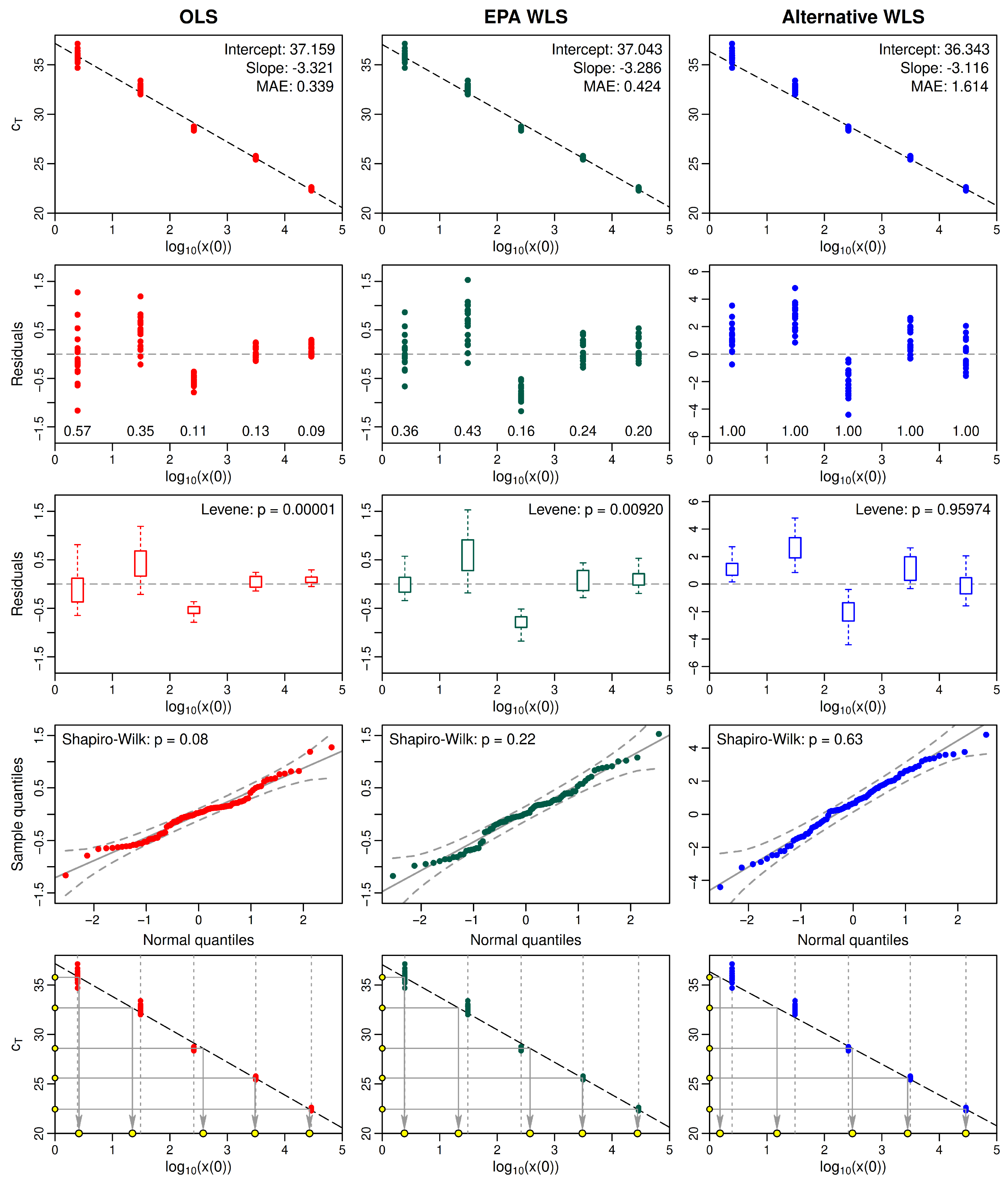
2.4. Fitting the Regression Model to Calibration Data

Estimates of intercept and slope parameters β 0 and β 1 are obtained by fitting Equation (19) to calibration data produced by measuring c T values for a set of different standards (calibrants), each with several replicates. Standards are solutions containing the target sequence at different concentrations that are prepared or measured in such a way that it is deemed reasonable to treat them as known. A potentially important source of systematic error in qPCR calibration is error in the TSC concentrations assigned to different standards. In practice, these concentrations are often estimated with ddPCR (e.g., EPA Draft Method C [52]). As we explain below in Section 3.2.3, they are, therefore, dependent on proper determination of the mean droplet volume for the particular laboratory instruments and assay mix employed by the lab performing the ddPCR analysis. In our experience, this determination is rarely performed; labs typically accept the default estimate of the mean droplet volume encoded in software supplied by the instrument manufacturer, which is known to be unreliable [53,54,55]. Since ddPCR concentration estimates are inversely proportional to the value of the mean droplet volume (Section 3.2.1), error in the estimated mean droplet volume can result in a meaningful error in the resulting estimate of TSC concentration in a  standard.
In addition to the problem of the accurate estimation of TSC standard concentrations, several purely statistical problems are encountered in fitting a linear regression model to the calibration data. For the estimates of β 0 (intercept) and β 1 (slope) to be valid, it is important to perform various quality control checks on the calibration data to determine if they exhibit excessive variability or a clearly nonlinear trend, or if a small number outliers are present that must be removed. If one wishes not only to obtain point estimates of β 0 and β 1 but also to estimate confidence intervals for them or test statistical hypotheses, then residuals of the fitted model must be examined carefully to assess the key assumptions of the type of regression analysis employed. This procedure often reveals that a different regression model is required, as briefly discussed later in this section.
The calibration data consist of a set of pairs ( u i , y i ) for i = 1 , 2 , 3 , , I , where u i is the log 10 -transformed value of the initial TSC concentration x i ( 0 ) in the i-th sample (that is, u i = log 10 ( x i ( 0 ) ) ), y i is the corresponding observed value of c T in sample i, and I is the total number of samples (“samples” here are replicates of the different standards, whose concentrations are assumed to be accurately known). In the typical case with equal replication, I is the number of different standards times the number of replicates per standard.
In classical linear regression, one assumes that the observed value of the response variable is a random variable that is the sum of two components: a predicted or “true” value that is a deterministic linear function of the predictor variable (in our case, u i ), and a random variable ξ i with mean zero that accounts for the discrepancy between the predicted and observed values. Let Y i be a random variable representing the observed value of the threshold cycle in the i-th sample, and let c ^ T i denote the corresponding predicted value. Using Equation (19), c ^ T i is given by
c ^ T i = β 0 + β 1 u i .
The random variable Y i , whose value y i is observed when c T is measured in sample i, is the sum of predicted value c ^ T i and random error ξ i . That is,
Y i = c ^ T i + ξ i = β 0 + β 1 u i + ξ i , i = 1 , 2 , 3 , , I .
We assume the ξ i are independent and have mean zero and finite variance, but we leave open the possibility that the variance of ξ i may be different for different standards. The set of I equations in Equation (30), together with assumptions regarding the mean and variance of ξ i , is the statistical model of the data.
To explain very briefly the process by which Equation (30) is used to estimate β 0 and β 1 , we will consider two different approaches, depending on whether one merely wishes to obtain valid estimates of these parameters and then use them to estimate initial copy number x 0 or log 10 ( x 0 ) (we will call this the simple estimation approach) or also wishes to estimate confidence intervals for the parameters or test statistical hypotheses (we will call this the statistically rigorous approach). Both approaches use the least-squares estimation framework and produce the same estimates, but the simple estimation approach makes no use of probability theory and requires no strong assumptions about statistical properties of errors. We will begin with the simple estimation approach, then indicate the additional assumptions that must be made and verified if one wishes to employ the statistically rigorous approach.
Both approaches use the quantity β 0 + β 1 u i as the predictor of response variable Y i for each value u i of the predictor variable. The difference between the observed value y i of response variable Y i and the corresponding predicted value β 0 + β 1 u i is used as a measure of error contained in the observed value y i (not the predicted value). To avoid confusing this type of error with random error ξ i , it is usually called the residual error or, simply, the residual. Thus, the residuals for observations i = 1 , 2 , 3 , , I can be expressed as
residual i = observed i predicted i = y i ( β 0 + β 1 u i ) .
The residual errors have two components: one due to errors in choosing values for β 0 and β 1 , and the other due to random errors ξ i , which are not observable.
In the ordinary least-squares (OLS) estimation framework, the goal is to find choices of β 0 and β 1 that minimize the sum Q ( β 0 , β 1 ) of squared residuals. For any values of β 0 and β 1 , this sum is given by
Q ( β 0 , β 1 ) = i = 1 I ( residual i ) 2 = i = 1 I [ y i ( β 0 + β 1 u i ) ] 2 .
Least-squares estimates of the intercept and slope parameters, denoted by β ^ 0 and β ^ 1 , are simply the values that minimize Q ( β 0 , β 1 ) and are easily found. The objective, then, is to minimize the contribution that errors in the values of β 0 and β 1 make to the total residual error, leaving random errors ξ i as the dominant contributors. The residuals should then be reasonable estimates of random errors ξ i if the underlying relationship between predictor and response variables truly is linear. With the simple estimation approach, it is unnecessary to make assumptions about the statistical properties of errors. In particular, we need not make assumptions about the specific probability distribution they come from, whether their variance is homogeneous for all u i , or even whether they are independent. This approach, then, is simply a “curve-fitting” approach.
The statistically rigorous approach to estimating β 0 and β 1 finds the estimates in exactly the same way but focuses on random variables Y i and ξ i and the probability distributions they are assumed to come from. It imposes several specializing assumptions about the statistical properties of errors ξ i that make it possible to estimate confidence intervals for β 0 and β 1 and, if desired, test statistical hypotheses about them. Specifically, the statistically rigorous approach assumes errors ξ i are independent and (approximately) normally distributed with constant mean zero and with a variance that is positive and finite for all i, and constant for all i corresponding to any given standard, but possibly different for different standards. If the qPCR analysis was performed correctly, the trend in the data should be well described by a straight line (as in Figure 4 above), in which case, the residuals should show no compelling evidence of serial correlation (which would violate the independence assumption). The normality assumption should be checked visually with a normal quantile–quantile plot (optionally supplemented with a formal test, such as the Shapiro–Wilk test) and, in our experience, usually is tenable. The simplest assumption regarding error variance is that it is homogeneous for all standards, in which case, the variance of the residuals should be homogeneous, as well. This property can be checked visually with a plot of residuals versus the log 10 -transformed standard concentration and a box plot (optionally supplemented with a Levene test for homogeneity) and often is dubious or clearly untenable.
Unless there is strong evidence to the contrary, the variance homogeneity assumption should be accepted as valid and OLS regression should be employed. If, however, variance is clearly not homogeneous across standards, weighted least-squares (WLS) regression is sometimes recommended (this is, in fact, the default method used in the spreadsheet workbook that accompanies EPA Draft Method C). With this type of regression, the squared residuals are multiplied by positive weights before summing. The weighted sum Q ( β 0 , β 1 ) of squared residuals is then given by
Q ( β 0 , β 1 ) = i = 1 I w i · ( residual i ) 2 = i = 1 I w i [ y i ( β 0 + β 1 u i ) ] 2
(e.g., [56], Section 2.1.3.1), where w i > 0 is the weight attached to the i-th squared residual. With the weights fixed, least-squares estimates of β 0 and β 1 are found by minimizing Q ( β 0 , β 1 ) , as with OLS regression.
Moving w i inside the brackets in Equation (33), Q ( β 0 , β 1 ) can be written in the equivalent form,
Q ( β 0 , β 1 ) = i = 1 I [ y ˜ i ( β 0 w i + β 1 u ˜ i ) ] 2 ,
where
y ˜ i = y i w i , u ˜ i = u i w i .
If we view y ˜ i as a response variable and w i and u ˜ i as predictor variables, then Equation (34) is just the sum of squared residuals for a two-predictor OLS regression model with response variable y ˜ i , predictor variables w i and u ˜ i , slope parameters β 0 and β 1 , and fixed intercept 0. The underlying model of the data is
Y ˜ i = β 0 w i + β 1 u ˜ i + w i ξ i ,
where the last term on the right is the error term. This two-predictor model is used to estimate β 0 and β 1 and their confidence intervals. The variance of the error term is w i σ i 2 , which can be made approximately constant for all i if the weights are chosen so that w i is inversely proportional to σ i 2 .
The residuals of the two-predictor model for observations 1 , 2 , 3 , , n are given by
residual i = y ˜ i ( β 0 w i + β 1 u ˜ i ) .
Once parameters β 0 and β 1 have been estimated, these residuals should be reasonable estimates of errors w i ξ i if the weights are chosen well, and they, therefore, should be approximately homogeneous over i. If so, valid confidence intervals for β 0 and β 1 can be estimated. However, because the variance of ξ i is often relatively low for high standards and high for low standards, greater weight will be attached to squared residuals for high standards than for low ones, potentially causing the fitted least-squares regression model to fit high standards better than low ones. As result, the accuracy of predicted target sequence copy numbers in samples with low concentrations may be lower than the accuracy at high concentrations (an example with real data is given below). In that case, if one is mainly interested in accurately estimating target sequence copy numbers in environmental samples and if some of these are likely to be low, then the use of OLS regression may be preferable.

2.5. Example: Comparing Statistical Properties of Fitted OLS and WLS Standard Curves

A fundamental principle of qPCR analysis is that measuring target-sequence copy numbers in environmental samples depends critically on a standard curve that has been fitted to a set of calibration data comprising pairs ( u i , y i ) of known log 10 -transformed initial copy numbers u i = log 10 ( x i ( 0 ) ) and corresponding measured threshold cycles y i for a set of standards with different concentrations of the target sequence. The fitted standard curve is linear and is, therefore, determined by its intercept and slope parameters β 0 and β 1 . The least-squares estimates of these parameters, when inserted in the inverted standard curve, determine the estimated target-sequence copy number for each c T value measured in an environmental sample. The purely statistical issue of how best to fit a standard curve to calibration data to obtain reasonable estimates of β 0 and β 1 is, therefore, of great importance in qPCR analysis but is not as simple as one might hope.
EPA Draft Method C has been used extensively in the United States for monitoring the E . c o l i contamination of aquatic habitats. A spreadsheet workbook distributed with this method performs various calculations that are required for assessing data quality, fitting standard curves, and calculating copy numbers in environmental samples. To simplify the use of the workbook by laboratory personnel with little statistical background, the current version of this workbook automatically uses WLS regression to fit standard curves to calibration data, without basing this choice of regression approach on a careful assessment of the assumptions of OLS and WLS regression or the resulting model fits. Additionally, the spreadsheet automatically employs as weights the known log 10 -transformed copy numbers for different standards, with no assessment of whether these weights successfully homogenize the variance of residuals for the fitted WLS model. The rationale for this choice of weights is that one often finds the variance of residuals to be higher for the lower standard concentrations than for the higher concentrations, so it is reasonable to think that standard concentrations might be approximately inversely proportional to the variance of the corresponding residuals. But like any other choice of weights, this choice requires careful assessment to determine whether it succeeds in homogenizing the variance of residuals and whether the resulting intercept and slope parameters perform better than (or as well as) those for standard OLS regression when used in Equations (22) or (23) for estimating copy numbers in samples.
We now consider an example with real qPCR calibration data that allows us to compare the performance of OLS and two types of WLS regression which use different weighting schemes, including the scheme used in the current EPA Method C workbook. The results of our comparison are specific to the particular data set we employ but illustrate the importance of assessing alternative regression models and their assumptions when fitting qPCR standard curves.
The data set we consider consists of six runs of a qPCR calibration study. Each run used five standards (i.e., five different known concentrations of a particular DNA target sequence), with three replicates of each. In each run, the threshold cycle c T was determined for each replicate of each standard, yielding six separate sets of calibration data. The spreadsheet workbook automatically runs preliminary quality-assurance checks to determine (among other things) whether the data sets for different runs are sufficiently consistent to be combined. In this example, the spreadsheet concluded that it was appropriate to combine the data from all six runs, yielding a composite data set with 18 replicates (six runs × three replicates per run) for each of the five standards. The workbook then used this composite data set to estimate intercept and slope parameters β 0 and β 1 and their 95% confidence intervals. EPA Draft Method C refers to the resulting standard curve as a “composite curve”.
We assessed three procedures for estimating β 0 and β 1 with these data:
  • Simple OLS regression;
  • WLS regression using the EPA Draft Method C weights;
  • WLS regression using alternative weights based on the data.
We will refer to these procedures as OLS, EPA WLS, and Alternative WLS regression. As mentioned above, the EPA WLS weights are the known log 10 -transformed copy numbers for the different standards. The Alternative WLS weights are 1 / s j 2 , where s j is the sample standard deviation of the 18 residuals for standard j in the OLS model or, equivalently, of the 18 measured c T values (e.g., [56], Section 2.1.3.1). We note that our parameter estimates and 95% confidence intervals for EPA WLS regression, computed with our own program written in the R programming language [57], agree exactly with results calculated by the EPA Draft Method C spreadsheet workbook.
The assumptions of the normality and variance homogeneity of residuals were assessed both visually and with formal statistical tests. Normality was assessed using quantile–quantile plots, supplemented with Shapiro–Wilk tests. Variance homogeneity was assessed using box plots, supplemented with Levene tests. The overall fit of the different regression models was quantified on the original measurement scale using the mean absolute error MAE, defined by
MAE = 1 n i = 1 I | residual i | ,
which avoids squaring the residuals and is, therefore, less sensitive to outliers than is the root mean squared error.
Figure 5 shows the results of our assessment. The first column of panels applies to OLS regression, the second to the EPA WLS regression, and the third to Alternative WLS regression. The first row of panels shows c T versus log 10 ( x 0 ) calibration data and fitted regression lines, the second shows residuals as defined by Equation (31) for OLS regression and by Equation (37) for WLS regression, the third shows corresponding box plots of the residuals, the fourth shows normal quantile–quantile plots of the residuals, and the last shows inverse predictions of log 10 ( x 0 ) for the five standards, based on means of the corresponding measured c T values and Equation (22).
Several interesting conclusions emerge from these results. The first row of panels suggests that all three regression models fit the calibration data well at high standard concentrations, but that the Alternative WLS model does not fit the data at the two lowest concentrations as well as the OLS and EPA WLS models do. The second and third rows of panels show that the variance homogeneity assumption for residuals is not tenable for either the OLS or EPA WLS models but clearly is for the Alternative WLS model. The first panel in the second row also shows that the standard deviations s j of c T values listed at the bottom of the panel (these are also the standard deviations of residuals for the OLS model) are smallest for the middle and highest standards and much larger for the two lowest standards. Because the Alternative WLS model weights residuals for each standard by 1 / s j 2 , residuals for the middle and highest standards are weighted most heavily and those for the two lowest standards are weighted least heavily. This is why the Alternative WLS model fits the middle and highest standards particularly well and the lowest standard particularly poorly. The fourth row of panels shows that the normality assumption is tenable for residuals of all three regression models. In the last row of panels, the means of the measured c T values for the different standards were inserted in the inverse prediction equation stated in Equation (22) to predict log 10 copy numbers for the standards. All of these predicted log 10 copy numbers should be close to the corresponding actual log 10 copy numbers in the standards if the calibration data are of good quality and the standard curve has been fitted well. Note that the OLS and EPA WLS models predict well at the lowest and two highest concentrations but noticeably worse at the two intermediate concentrations. The Alternative WLS model predicts well at the three highest concentrations but noticeably worse at the two lowest concentrations. These patterns in row 5 are consequences of the patterns in row 1 and result from the choice of regression model and weights used to fit the standard curve.
We conclude that, in this particular example using real data, it is not clear that using either type of WLS regression model is preferable to using the OLS model. The OLS and EPA WLS models performed similarly with regard to predicting TSC concentrations across the entire range of standards, but in neither case was the variance of residuals homogeneous, as required for proper parametric estimation of confidence intervals or tests of statistical hypotheses. By contrast, the Alternative WLS regression model successfully homogenized the variance of residuals but predicted concentrations less accurately than the OLS or EPA WLS models at low concentrations. When such cases arise in environmental applications, it seems more important to obtain accurate estimates of sample TSC concentrations across the entire range of standards at the cost of some heterogeneity of the regression residuals, than it is to resolve the problem of variance heterogeneity at the cost of inaccurate estimates for low TSC concentrations.
These conclusions, of course, apply only to the particular example considered. More generally, we may tentatively conclude that neither the desirability of using WLS regression nor the best weighting scheme to employ should simply be assumed; both choices should be assessed on a case-by-case basis. Because of the importance of proper fitting of the standard curve in qPCR analysis, we think a more thorough statistical assessment of alternative fitting methods is needed. Such an assessment, however, is beyond the scope of the present study.

3. Droplet Digital PCR

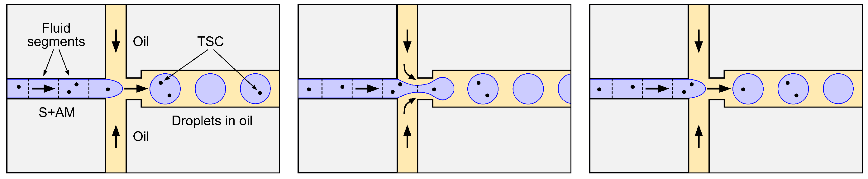
3.1. A Brief Overview of ddPCR

As in the case of qPCR, numerous protocols are available for ddPCR analysis of environmental samples. (An example of a ddPCR workflow that has been widely used in the state of Michigan for monitoring SARS-CoV-2 concentrations in wastewater is presented in Appendix C. Kokkoris et al. [58] give another example of a ddPCR protocol for environmental samples and provide an interesting assessment of the effects of modifying various protocol parameters.) Regardless of the protocol used, the first step in ddPCR analysis is sample preparation, which releases the genetic material contained in cells of the target taxon and cleans the sample to varying degrees for subsequent analysis. The methods used are the same as those described for qPCR in Section 2.1 and will not be repeated here.
Droplet digital PCR (ddPCR) is an endpoint form of PCR analysis where each sample is partitioned into roughly 10,000–20,000 nanoliter-size droplets, each functioning as a separate PCR reactor. As in qPCR, the prepared sample is combined with an assay mix containing primers, probes, dNTPs, DNA polymerase, and other constituents, with primers and probes binding specifically to the target sequence of DNA. But unlike qPCR, the fluorescence of droplets is not monitored in real-time; it is assessed only once, after the number of amplification cycles is large enough so droplets that fluoresce above background can be reliably distinguished from those that do not (typically, 40–60 cycles). An individual droplet will fluoresce above background if and only if it originally contained one or more copies of the target DNA sequence (which was then amplified). As will be shown in Section 3.2, the original concentration of the target sequence can be estimated from two simple pieces of information: the observed proportion of droplets that did not fluoresce above background and the mean droplet volume.
In order to understand how ddPCR works, it is essential to have a basic idea of the manner in which droplets of the mixture of prepared sample and ddPCR assay mix are created. Some of the details vary between different ddPCR systems, but the process is as follows for the Bio-Rad® QX200TM PCR system. Very briefly, an instrument called a droplet generator uses pressurized air to push 20 μL of aqueous S+AM and 60 μL of a special oil through three separate microchannels (width and depth typically less than 100 μm) in a plastic chip. Oil flows through two of the microchannels and S+AM through the third. The two oil microchannels join the S+AM microchannel from opposite sides at a common point (Figure 6). As the flowing oil and S+AM merge, the fact that the two liquids are immiscible becomes important: Instead of mixing, droplets of S+AM are sequentially pinched off by oil flowing in from opposite sides of the S+AM microchannel, then remain suspended within the oil as it flows through an outflow microchannel. This process partitions the 20 μL of S+AM into roughly 20,000 nanoliter-size droplets, each with a volume of approximately 1.0 nL (the actual volume is somewhat variable but, typically, is closer to 0.8 nL [53,54,55]).
When nearly the entire 20 μL of S+AM has been processed by the droplet generator, the emulsion of aqueous droplets in oil is transferred to a multi-well plate and placed on a thermocycler for PCR amplification, which occurs separately in each droplet that contains one or more copies of the target sequence. Once amplification is complete, the plate is placed on an instrument called a droplet reader. The emulsion in each well is aspirated sequentially by a needle and passed through a microchannel where the droplets pass, one at a time, through a beam of light at the excitation wavelength for the reporter being employed. The fluourescence of the droplet-in-oil emulsion at the emission wavelength of the reporter is continuously monitored. Software for the droplet reader employs an automated peak-detection algorithm that assesses each putative fluorescence peak to determine whether to accept it as corresponding to a valid droplet, and the fluorescence amplitude of each accepted peak is recorded.
Even droplets that contain no TSC may have a positive but small fluorescence amplitude, so the analyst must set a threshold level that reliably separates flourescence amplitudes in positive control droplets from fluorescence amplitudes in negative control and no-template control droplets. Software accompanying the droplet reader uses this threshold to classify each S+AM droplet as either positive (fluorescing above the threshold) or negative (not fluorescing above the threshold) for the target sequence. The software then uses the observed proportion of negative droplets and an assumed mean droplet volume to calculate an estimate of the target sequence concentration as TSC per 20 μL of S+AM (as discussed below, the reported concentration will require adjustment if there is a meaningful difference between the mean droplet volume coded into the instrument software and the actual mean volume of droplets produced by the particular droplet generator and master mix used in a given study).
Depending on the purpose of the study, it may be necessary to convert concentrations in the S+AM to concentrations in the original field samples, accounting for all concentration and dilution steps during sample preparation and analysis. Unlike qPCR, ddPCR does not require a standard curve and does not depend on estimates of amplification efficiency. These are important advantages.

3.2. Basic Equations of the ddPCR Process

As discussed in Section 3.1, the concentration of the target sequence in a sample can be estimated with ddPCR using only the proportion of negative droplets, as determined by the droplet reader, and the mean droplet volume. We now show why this is true. Our exposition is somewhat more detailed than the various expositions we have encountered in the literature and on instrument manufacturer and vendor websites, since we feel it is important to be aware of the key assumptions and approximations underlying the theory and the manner in which the main results can be logically derived.
The key result to be justified is the formula typically used in ddPCR analysis to estimate the concentration of TSC in the S+AM (number per volume of S+AM):
C = log e ( m 0 / m ) / v ¯
(e.g., [40], pp. 54–55). Here, C is the TSC concentration in the S+AM, m is the total number of accepted droplets scanned by the droplet reader, m 0 is the number of these droplets that were classified as negative (i.e., that did not fluoresce above background and, therefore, contained no TSC), m 0 / m is the proportion of droplets that were negative, and v ¯ is the mean droplet volume. It is important to be aware that the mean droplet volume depends on the type of droplet generator and master mix used (and, possibly, on other factors that have not yet been assessed), with most of the reported optically-measured values ranging from 0.7 and 0.9 nL [53,54,55,59].
In our derivation of Equation (38), we will assume that S+AM, oil, and droplets suspended in oil all move through the various microchannels shown in Figure 6 via plug flow. Thus, each type of fluid is assumed to move as if on a conveyor belt, and any arbitrary segment of the fluid (and any TSC it contains) remains intact as it moves through the microchannel, like a plug or piston. Consistent with the plug flow assumption, it is useful to think of the stream of S+AM flowing through the sample microchannel as consisting of a sequence of disjoint segments, each having approximately the same volume and each becoming a single droplet when pinched off by inflow of oil from the two oil microchannels, as illustrated in Figure 6.

3.2.1. Estimating the TSC Concentration

We begin with several assumptions regarding probabilistic properties of the number of TSC in different segments of the S+AM as it flows through the sample microchannel, prior to the inflow of oil (Figure 6):
  • Before being drawn into the sample microchannel, the S+AM is homogeneous (well mixed) in the sense that any given TSC that was present in the original sample is equally likely to be contained in any subset of the S+AM of fixed volume v V , where V is the total S+AM volume (≈20 μL).
  • The droplet generator partitions the entire S+AM volume V (or nearly so) into a large number n of droplets ( n 20 , 000 is typically assumed) of variable but similar volumes.
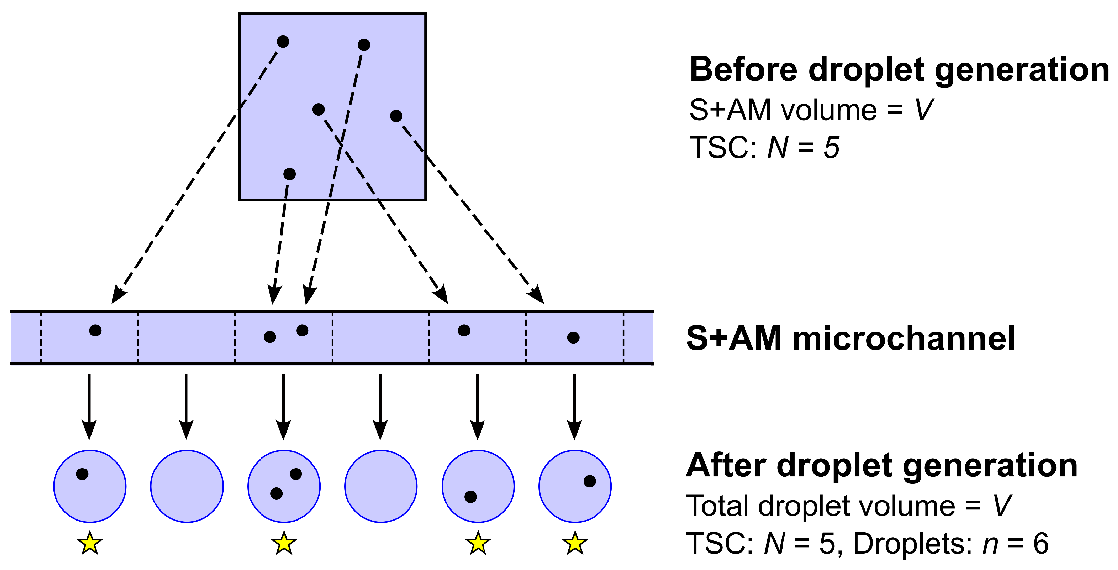
  • The process by which the N TSC present in the S+AM are allocated to the n disjoint segments of S+AM flowing through the sample microchannel, and, hence, to the n resulting droplets, is a stochastic partition process equivalent to independent random allocation of N objects (the TSC) to n boxes (the segments or droplets) labeled 1 , 2 , , n , where each object has probability π j of being allocated to box j (Figure 7).
  • The probability π j that any given TSC is allocated to S+AM segment or droplet j is simply the fraction of S+AM volume V that the segment or droplet contains, so that
    π j = v j / V , j = 1 , 2 , , n .
  • In order to arrive at the simple standard formula for TSC concentration C in the S+AM stated in Equation (38), we must make the additional assumption that the volumes of different droplets are similar enough so the approximation,
    v j v ¯ , j = 1 , 2 , , n ,
    is adequate, in which case, it follows that
    π j v ¯ / V : = π ¯ , j = 1 , 2 , , n .
These assumptions imply that the numbers Z 1 , Z 2 , , Z n of TSC in droplets (and segments) 1 , 2 , , n are random variables that jointly have a multinomial distribution M n ( N ; π 1 , π 2 , , π n ) with probability function
Pr ( Z 1 = z 1 , Z 2 = z 2 , , Z n = z n ) = N ! z 1 ! z 2 ! z n ! π 1 z 1 π 2 z 2 π n z n N ! z 1 ! z 2 ! z n ! π ¯ N ,
where realized values z 1 , z 2 , , z n are constrained to sum to N and we used (in the second step) the assumption that π j π ¯ for every droplet j. Symbols and associated dimensions employed in the qPCR equations here and below are summarized in Table 3.
An important property of the multinomial distribution (and the partition process it represents here) is that the numbers of objects allocated to different boxes are not independent, because the numbers of objects and boxes are fixed and finite (e.g., in the extreme case where all N objects happen to be allocated to a particular box j , none can be allocated to any other box). The correlation between the numbers of TSC in any two S+AM droplets is negative and is given by
Cor ( X i , X j ) = t π i π j t ( 1 π i ) ( 1 π j ) , i j
(e.g., [60]). Under our assumptions, then,
Cor ( X i , X j ) π ¯ / ( 1 π ¯ ) = 1 / ( n 1 ) .
Thus, for n = 10 k with k 3 , we find that Cor ( X i , X j ) 10 k . It follows that the between-droplet correlation in TSC counts is negligible for n > 1000 , which clearly holds for typical ddPCR applications with n 20 , 000 .
The key implication of this result is that, because the number n of droplets is so large, the numbers of TSC in different droplets can be assumed to be independent random variables, even if the entire 20 μL of S+AM is partitioned to produce the droplets. Under the independence assumption, the number of TSC in each droplet when it was created by the droplet generator has the same probability distribution and is not influenced by the number of TSC in any other droplet. This distribution is easily shown to be binomial with “success” probability π = 1 / n and number of “trials” N (hence, the mean number of TSC per droplet = N π = N / n ), but as we will see shortly, it is only necessary to determine the probability that any given S+AM droplet contains no TSC; the rest of the binomial distribution plays no role in estimating the concentration of TSC, nor do we have any way of knowing the number of TSC that were present in individual positive droplets when they were created.
The probability P 0 that any given S+AM droplet contains no TSC is simply the probability that none of the N TSC was allocated to the segment from which the droplet was formed. Under the independence assumption, and using Equation (39), P 0 is given by
P 0 = ( 1 π ) N = ( 1 1 / n ) N .
Taking the logarithm of both sides and solving for N yields the following formula for the total number of TSC in the S+AM:
N = log e ( P 0 ) log e ( 1 1 / n ) .
This formula actually holds for logarithms with respect to any base (provided the base is the same in the numerator and denominator), but the derivation of Equation (38) is simpler with base e.
The concentration C of TSC in the S+AM is the number N of TSC divided by the total volume V of S+AM. That is,
C = N V = log e ( P 0 ) V log e ( 1 1 / n ) = log e ( P 0 ) i = 1 n v i log e ( 1 1 / n ) .
Because n is so large (≈20,000), 1 / n is very small (≈0.00005). To a very good approximation, then, we may assume
log e ( 1 1 / n ) = 1 / n
(MacLaurin series with remainder). Equation (47) then becomes
C = log e ( P 0 ) ( 1 / n ) i = 1 n v i = log e ( P 0 ) v ¯ .
In practice, not all of the n droplets into which the S+AM was partitioned are scanned and accepted by the droplet reader. Therefore, let m < n denote the number of droplets that are scanned and accepted. To obtain a valid estimate of the TSC concentration in the S+AM with this subset of droplets, the m droplets in the subset must be a representative sample of the total number n of droplets in the S+AM. Because both m and n typically are large (> 10 4 ) and there is no apparent source of bias in determining which droplets will be read, it is reasonable to assume this requirement is satisfied. The following corollary properties then hold:
  • The probability P 0 that a randomly chosen droplet from the m scanned and accepted droplets contains no TSC is the same as the probability P 0 that a randomly chosen droplet from the full set of n droplets contains no TSC. That is, P 0 = P 0 .
  • The ratio N / m of TSC to droplets in the m scanned and accepted droplets is the same as the ratio N / n in the full set of n droplets. That is, N / m = N / n .
  • The mean droplet volume v ¯ in the m scanned and accepted droplets is the same as the mean droplet volume v ¯ in the full set of n droplets. That is, v ¯ = v ¯ .
  • It follows from properties 1 and 2 that, to a very good approximation, the ratio N / V of the cumulative number N of TSC in the m scanned and accepted droplets to the cumulative volume V of those droplets is the same as the ratio N / V of the cumulative number N of TSC in the total number n of droplets (and in the S+AM) to the total volume V of those droplets (and of the S+AM). That is,
    C = N V = N V = C ,
    where C is the TSC concentration in the combined n droplets (and in the S+AM) and C is the combined TSC concentration in the m droplets scanned and accepted by the droplet reader.
Properties 1, 3, and 4 imply that we may substitute P 0 for P 0 and v ¯ for v ¯ in Equation (49), and that, to a very good approximation, C = C . The formula for the concentration C of TSC in the S+AM, given by Equation (49), can then be written as
C = C = log e ( P 0 ) / v ¯ = log e ( P 0 ) / v ¯ .
As in the case of qPCR, it is often desirable to convert this concentration in S+AM to the corresponding concentration in the original sample or standard. The process for doing so is the same: We multiply the concentration in S+AM by a dimensionless dilution correction factor F that adjusts it appropriately to account for sample dilution and concentration steps that occurred during sample processing and analysis (for an example, see [53]). The concentration C sample in the original sample is, therefore, given by
C sample = F C = log e ( P 0 ) F / v ¯ .
In order to use Equation (51) to estimate the TSC concentration in the S+AM, the values of parameters v ¯ and P 0 must be determined. The value of P 0 can be determined statistically using a maximum-likelihood estimator (Section 3.2.2). An estimate of v ¯ is coded into software supplied by instrument manufacturers, but such universal estimates have been found to be unreliable. More specifically, it has been shown by multiple laboratories and metrology organizations around the world that the value of v ¯ differs meaningfully for different droplet generators and master mixes [53,54,55]. Thus, while it is true that ddPCR does not require a standard curve, it does require calibration. The recommended procedure is to estimate v ¯ for each combination of droplet generator and master mix used in a particular laboratory by measuring droplets under a microscope in accordance with published protocols (e.g., [53,54]). A simpler alternative, which we propose in Section 3.2.3, is to employ one-point calibration using a certified reference material (CRM) with known TSC concentration.
Before discussing the estimation of v ¯ and P 0 , we perhaps should explain why we have not mentioned what is referred to as “Poisson statistics” in ddPCR documentation on manufacturer websites. In the context of problems like the one we are considering, the standard theory of spatial Poisson stochastic processes does not apply, because TSC are allocated to droplets by partitioning a fixed number of TSC. Instead, the Poisson distribution arises as an approximation to the binomial distribution, which, in turn, is an approximation to the underlying multinomial distribution. The binomial approximation should be very good, because the extremely large number n of droplets ensures that the correlation between TSC numbers in different droplets is negligible, and variation in droplet size (hence, π j ) is minimal (see Section 3.2.2). Because n is so large, the Poisson approximation also should be fairly good, provided the average number of TSC per droplet ( N / n ) is less than about 10 (e.g., [61], p. 64). However, it is actually only necessary for the Poisson approximation to P 0 to closely approximate the corresponding binomial probability given by Equation (45) with P 0 = P 0 . The Poisson approximation to P 0 is
P 0 = e N / m = e N / n .
Numerical analysis of the difference between the binomial probabiity in Equation (45) and the Poisson approximation to it in Equation (53) show that for n 10 , 000 , the difference is less than 0.00002 for all values of TSC number N 1 . However, we see no reason to use the Poisson approximation instead of the binomial probability, which is simple to compute and has a more transparent relationship with the underlying multinomial distribution.

3.2.2. Estimating the Probability That a Droplet Has No TSC

We now outline the statistical theory for estimating P 0 , the probability that any given scanned droplet contains no TSC, based on droplet-reader results for a large number m < n of scanned and accepted droplets. Let Y j be a binary (Bernoulli) random variable indicating whether droplet j is negative ( Y j = 0 ) or positive ( Y j = 1 ) when scanned. Thus, for each droplet j, we will have either Y j = 0 , if the droplet contained no TSC when it was formed, or Y j = 1 , if the droplet contained one or more TSC when it was formed (which were then amplified by PCR before being scanned by the droplet reader). The probability distribution of Y j can, therefore, be expressed as
Y j = 0 , with probability P 0 1 , with probability 1 P 0
for all j.
Recalling the independence assumption justified by the multinomial argument presented in Section 3.2.1, we may treat Y 1 , Y 2 , Y 3 , as independent random variables. Without loss of generality, we may interpret Y j = 0 as a “success” and Y j = 1 as a “failure”. Then, by definition of the binomial distribution, the number of negative droplets in m accepted droplets has a binomial distribution with success probability P 0 and number of trials m. (Note: the number of positive droplets is also binomial but with success probability 1 P 0 ; we see no valid reason to approximate the binomial with a Poisson distribution, as is sometimes done, since this inevitably introduces additional error and all the necessary statistical theory is available for the binomial distribution.) It follows that the likelihood L ( P 0 ) of obtaining the observed number m 0 of successes in m Bernoulli trials ( 0 m 0 m ) is given by
L ( P 0 ) = m m 0 P 0 m 0 ( 1 P 0 ) m m 0 .
We wish to choose P 0 to maximize this likelihood. Note that L ( 0 ) = 0 = L ( 1 ) and L ( P 0 ) > 0 for all P 0 ( 0 , 1 ) , suggesting there is an interior maximum. The log-likelihood function ( P 0 ) : = log e ( L ( P 0 ) ) is given by
( P 0 ) = const + m 0 log e ( P 0 ) + ( m m 0 ) log e ( 1 P 0 ) .
Differentiating ( P 0 ) with respect to P 0 and setting the derivative to zero (and confirming the second derivative at the implied value of P 0 is negative), we find that the maximum-likelihood estimator P ^ 0 for P 0 is
P ^ 0 = m 0 / m .
Thus, P ^ 0 is simply the proportion m 0 / m of negative droplets among the m droplets accepted by the droplet reader. Values of both m 0 and m are automatically reported by the software that accompanies the ddPCR droplet reader.
Generally speaking, the two best methods for estimating a 95% confidence interval for a binomial success probability like P 0 , in terms of coverage probability and expected width, are the Wilson method and the Agresti–Coull method [62]. Simulation studies have shown that unless the number of trials is very large (≫100), the traditional Wald (asymptotic) method typically yields confidence intervals for a binomial probability that correspond to a true confidence level that is much lower than the nominal 95% (meaning that the actual probability that the true value of P 0 lies within the interval is much less than the nominal 95%) and, hence, are much narrower than they should be [62,63]. But, because the total number m of accepted droplets is so large in ddPCR applications (typically, m > 10,000), Wald confidence intervals tend to be very similar to the Wilson and Agresti–Coull intervals (see the examples below in Section 3.2.4).
Substituting maximum-likelihood estimator P ^ 0 for P 0 , Equations (51) and (52) become
C S + AM = log e ( m 0 / m ) / v ¯
C sample = log e ( m 0 / m ) F / v ¯ .
These formulas allow us to estimate the unknown concentration of TSC in the S+AM or in a sample, once we have determined the mean droplet volume v ¯ and, in the latter case, the dilution correction factor F. Note that when applying these formulas, the volume unit of v ¯ determines the volume unit of C S + AM and C sample . Thus, if we wish to express these concentrations in gene copies per μL (GC/μL), then v ¯ must be expressed in μL instead of nL (note: estimates of v ¯ usually are reported in nL).
Equations (58) and (59) provide point estimates of TSC concentration but give no estimate of their level of uncertainty. As we noted regarding qPCR estimates of TSC copy number per reaction, there are two main sources of this uncertainty: one due to error in the estimate of v ¯ used, and the other due to statistical error in estimating P 0 by m 0 / m .
Regarding the first source, let v ¯ ˜ and v ¯ denote the estimated and true values of the mean droplet volume, and suppose v ¯ ˜ contains proportional error η drop v ¯ so that
v ¯ ˜ = ( 1 + η drop ) v ¯ .
Then, the estimated sample TSC concentration C ˜ sample based on v ¯ ˜ is related to the concentration C sample based on the correct value v ¯ as
C ˜ sample = log e ( m 0 / m ) F v ¯ ˜ = log e ( m 0 / m ) F ( 1 + η drop ) v ¯ = C sample 1 + η drop .
Thus, the proportional error in the estimated TSC concentration in a sample is the inverse of the proportional error in the estimate mean droplet volume. That is,
C ˜ sample C sample = 1 1 + η drop .
(The same relationship holds for the ratio of C ˜ S + AM to C S + AM .) This relationship indicates that overestimates of the mean droplet volume encoded in droplet generator software, as have been well documented in the past, will result in systematic underestimates of sample concentrations. For example, if the original nominal value of 1.00 nL were used for the mean droplet volume and the actual value is 0.80 nL, then the estimated sample concentration C ˜ sample would be about 83% of the correct value, or 17% too low. If an estimate of 0.85 nL were used instead 0.80 nL, C ˜ sample would be about 95% of the correct value, or 5% too low. Clearly, it is very important to have an accurate estimate of v ¯ .
The other source or error in C ˜ sample can be addressed by obtaining estimates of the lower and upper 95% confidence limits for C S + AM or C sample . One way to do this is by substituting the upper and lower 95% confidence limits (respectively) for P 0 in Equations (58) or (59) (another way is by using bootstrapping [64]). As noted above regarding the confidence limits for P 0 , the total number m of scanned droplets is large enough so the Wilson, Agresti–Coull, and Wald confidence intervals typically will be very similar. Alternatively, we can estimate confidence limits directly for C S + AM or C sample by bootstrapping; e.g., using the percentile or BC a algorithm of Efron and Tibshirani [64]. Because m is so large, the confidence limits estimated by these algorithms typically will be very similar to each other, as well as to those based on the confidence intervals for P 0 just mentioned (see the examples in Section 3.2.4 below).
These confidence limits do not account for variation in droplet volume, which, in any case, cannot be quantified unless one can accurately measure the volumes of individual droplets. Currently, the only practical method we know of for estimating individual droplet volumes is the optical microscopy imaging method [53,54,55]. Estimates of the mean and standard deviation of droplet volume obtained in this way can be used to assess the plausibility of treating the sample mean droplet volume v ¯ as a constant, as well as the plausibility of the related assumption that, to a good approximation, v j = v ¯ and hence, π j = π ¯ for all droplets j that were required in deriving the simple standard formula for TSC concentration C in Section 3.2.1.
Toward this end, let us assume the droplets generated from the S+AM in a particular plate well have true mean volume μ v , and let v ¯ m denote the sample mean calculated for a set of m droplets whose individual volumes were estimated with optical microscopy imaging. By the strong law of large numbers, v ¯ m μ v with probability one as m . But, for any finite m, there will be error in estimating μ v by v ¯ m . Denoting the relative error by | v ¯ m μ v | / μ v , we ask how likely it is that relative error | v ¯ m μ v | / μ v > δ , where δ is a small positive number ( 0 < δ < 1 ). By Chebychev’s inequality,
P | v ¯ m μ v | / μ v > δ 1 m CV δ 2
(see Appendix D), where P { x } denotes the probability of event x and CV is the coefficient of variation of droplet volume. Dagata et al. [54] report CV estimates ranging from 0.0042 to 0.0096 for two different DNA sources and two different master mixes. For a human genomic DNA source and a master mix containing dUTP (deoxyuridine triphosphate), they report a CV of 0.0046. Rounding this value up to 0.005, and choosing δ = 0.1 and m = 10 , 000 , we find that
P | v ¯ m μ v | / μ v > 0.1 2.5 × 10 7 ,
and for a single droplet ( m = 1 ),
P | v j μ v | / μ v > 0.1 2.5 × 10 3 .
Thus, the coefficient of variation of droplet size is sufficiently small, and the number m of accepted droplets is sufficiently large, so it is reasonable to expect deviations of v j from μ v that are more than 1/10-th as large as μ v to be rare, and deviations of v ¯ m from μ v that are more than 1/10-th as large as μ v to be extremely rare.
An important property of Equations (58) and (59) is that estimates C S + AM and C sample of TSC concentration depend only indirectly and weakly on the efficiencies of amplification and fluorescence. Because ddPCR is based on an endpoint reaction, amplification and fluorescence only need to be sufficient to eventually produce detectable above-threshold fluorescence in droplets that initially contained one or more TSC. Therefore, in marked contrast to qPCR, ddPCR is relatively insensitive to sample constituents that interfere with amplification or fluorescence, as long as they do not fully block these processes. This property has been confirmed empirically (e.g., [20]).

3.2.3. Estimating the Mean Droplet Volume

Methods for estimating mean droplet volume v ¯ by optical microscopy imaging are detailed by several authors [53,54,55]. These methods are relatively straightforward and, aside from standard ddPCR instrumentation and supplies, require only a high-quality research microscope with a digital imaging system. Košir et al. [55] found that mean droplet volume showed statistically significant and meaningful differences for different droplet generator models and different master mixes, and they, therefore, recommended that “to accurately determine copy number, the droplet volume should be measured for all possible droplet generators and master mixes used in a laboratory.” In our experience, however, this admonition is routinely ignored by ddPCR users in the biological and environmental sciences.
A possible alternative method for determining the appropriate mean droplet volume for the specific combination of droplet generator and master mix used in a particular lab is to employ a CRM as a calibration standard. A CRM is simply a sample whose TSC concentration has been estimated by some other method (e.g., chamber-based digital PCR) that is trusted sufficiently so it is thought reasonable to consider the estimated concentration known. Once m 0 and m have been determined for a CRM, the only unknown in Equations (58) and (59) is v ¯ . The appropriate value of v ¯ for a particular droplet generator and master mix can then be estimated as the value that causes the concentration calculated with Equation (38) to match the known TSC concentration of a CRM. Rearranging Equation (59), this value is given by
v ¯ = log e ( m 0 / m ) F / C ˜ sample ,
where C ˜ sample is the estimated TSC concentration in the CRM (expressed in the same volume unit as v ¯ ), F is the dilution correction factor, and m 0 and m are the number of negative droplets and total number of droplets reported when the CRM is analyzed. Aside from ddPCR instrumentation and supplies, this method requires only the purchase of a CRM. It depends critically on the accuracy of the certified concentration, which is also true of standard curves in qPCR analysis. A variety of CRMs are currently available from, for example, the Joint Research Centre’s Institute for Reference Materials and Measurements (JRC-IRMM) and the American Oil Chemists’ Society (AOCS). This method is much simpler and much less time-consuming than the optical microscopy method, but its validity has not yet been assessed.
Once the mean droplet volume for a particular combination of droplet generator and master mix has been determined, TSC concentrations for samples processed with the same droplet generator and master mix can be calculated either by using Equation (38), with the value of v ¯ that was determined and the values of m 0 and m reported by the instrument software, or by multiplying the concentration reported by the instrument software by the ratio v ¯ soft / v ¯ meas , where v ¯ soft is the value of v ¯ used by the instrument software and v ¯ meas is the value determined by optical microscopy or calibration with a CRM. If the instrument software does not report the assumed mean droplet volume v ¯ soft , it can be determined from the values of m 0 , m, and C reported by the instrument software for one or more samples; if these values are inserted on the right side of Equation (66), the calculated mean droplet volume will be v ¯ soft (possibly with a small roundoff error).
The effect of error in estimated CRM concentration C ˜ CRM is to create error in the estimate of mean droplet volume, which, in turn, creates error in concentration estimates for field samples. To assess the magnitude of this error, suppose the estimate of CRM concentration C ˜ sample (i.e., the certified concentration) contains proportional error ( 1 + η CRM ) C CRM , where C CRM is the correct CRM concentration. The resulting estimate v ¯ ˜ of mean droplet volume is then
v ¯ ˜ = log ( m 0 / m ) ( 1 + η CRM ) C CRM = v ¯ 1 + η CRM .
In turn, the resulting estimate of sample TSC concentration is
C ˜ sample = log e ( m 0 / m ) F v ¯ ˜ = ( 1 + η CRM ) C sample .
It follows that
C ˜ sample C sample = 1 + η CRM .
As in the case of qPCR estimates of TSC copy numbers per reaction, the proportional error in calibration standards is passed on unaltered to estimates for field samples, underscoring the importance of minimizing error in estimating the TSC concentration in CRMs. The alternative method of estimating v ¯ by optical microscopy imaging avoids the issue of CRM concentration accuracy but is much more time consuming and also involves meaurement error.

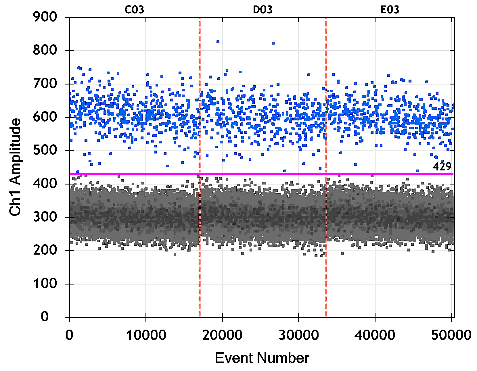
3.2.4. Example: Droplet Classification and Estimating the TSC Concentration

Figure 8 shows a plot of fluorescence amplitude (vertical axis) versus event or accepted droplet number (horizontal axis) created by Bio-Rad’s QuantaSoftTM software (version 1.7.4). In this example, three replicates of a positive control for the human-associated Bacteroidales genetic marker (target sequence) HF183 were analyzed with ddPCR. The horizontal magenta line at amplitude 429 on the vertical axis is the manually-set threshold fluorescence level used to classify droplets as positive (fluorescence amplitude greater than the threshold) or negative (fluorescence amplitude not greater than the threshold). Blue and gray dots are droplets classified as positive and negative, respectively. Sample well labels are listed at the top of the figure; classified droplets for different wells are separated by vertical dashed lines.
The numbers of negative droplets ( m 0 ) and all droplets (m) for each of the three wells shown in Figure 8 are shown in Table 4. Also shown are the maximum-likelihood estimates of binomial probability P 0 calculated with Equation (57), the estimated concentration C of the HF183 marker in S+AM calculated with Equation (58), three types of 95% confidence intervals for P 0 (computed with function binom.confint() in R package binom [65]), and six types of 95% confidence intervals for C (bootstrap confidence intervals were computed with function boot.ci() in R package boot [66] and function bcanon() in R package bootstrap [67]). Note that with one exception, the upper and lower 95% confidence limits for C are very similar for all types of confidence interval. The one exception is that the lower 95% confidence limits reported by Bio-Rad’s QuantaSoft software are consistently greater than the lower limits for the other types of confidence interval by more than 1.0  GC/μL (the QuantaSoft limits are based on a Poisson approximation to the actual binomial distribution, but the software documentation does not state which of the many methods for estimating Poisson confidence intervals is used). The mean droplet volume supplied by the instrument manufacturer ( v ¯ = 0.85 nL = 8.5 × 10 4  μL) was used in all calculations because no estimate was available for the specific combination of droplet generator and master mix used.

4. Discussion

Our review and assessment of the theoretical underpinnings of qPCR and ddPCR methods for estimating target sequence copy numbers and concentrations in water samples support the conclusion that both methods are sound. However, careful attention must be paid to specific details to ensure that the estimates obtained are accurate and precise. These key details differ between qPCR and ddPCR.
In the case of qPCR, it is particularly important to reduce any significant PCR inhibition by sample constituents, since qPCR copy number estimates depend strongly on the rate of amplification (amplicons produced per DAE cycle) and, therefore, are very sensitive to amplification efficiency. It is also important to ensure the proper choice and fitting of the regression model for the standard curve, including the assessment of potential outliers and potential nonlinearity. If one wishes to estimate confidence intervals for the slope or intercept parameters (e.g., for quality assurance purposes) or estimate confidence intervals for copy-number estimates produced by inverse prediction, then the statistical assumptions of the regression model must be carefully assessed. If any of these assumptions are not tenable, an alternative model must be chosen and assessed. This model selection process is nontrivial for three main reasons:
  • Over the range of standards typically required for analysis of water samples, the variance of measured c T values often differs markedly for different standards, meaning that the c T values are heteroskedastic. In such cases, the variance homogeneity assumption of classical OLS regression is not tenable.
  • One way to address heteroskedasticity is by employing WLS regression. However, any choice of weights must be carefully assessed to ensure it succeeds in homogenizing the variance in c T residuals.
  • Even if weights can be found so that WLS regression successfully homogenizes the variance of residuals, the resulting intercept and slope parameters may exaggerate errors in predicted sample copy numbers at low concentrations, due to heavier weighting of residuals for high concentrations, where c T values typically are less variable.
In the case of ddPCR, an important but commonly ignored issue is that the mean droplet volume—to which concentration estimates are quite sensitive—is known to differ meaningfully for different combinations of droplet generator and master mix. The fact that mean droplet volume is not constant across different instruments and assay mixes implies that no universal estimate of this critical parameter (e.g., a single value coded into instrument software by the instrument manufacturer) should be trusted. Instead, it is advisable to determine the appropriate mean droplet volume for the specific combination of droplet generator and master mix being used for a particular study, either by optical microscopy or by calibration with a CRM.
Both qPCR and ddPCR are potentially appropriate for many of the same types of analysis in studies of aquatic systems and may, therefore, be viewed as alternatives that one must choose between. With this choice in mind, we now summarize what we see as the main advantages and disadvantages of qPCR and ddPCR. Our comparison of the methods is structured around six groups of properties: cost, sample turnaround time, calibration, inhibition, limits of quantification, and simplicity (Table 5). Basu [9] provides an alternative comparison of these methods (which we recommend to the reader) that considers some of the same properties, but several others, as well. For the properties that both comparisons consider, our views regarding the advantages and disadvantages of qPCR and ddPCR largely agree with those of Basu [9].
Cost. The instrument and per-sample costs for ddPCR are substantially higher than those for qPCR at the time of this writing, but we expect both types of cost to become more similar to those for qPCR in the future.
Sample turnaround time. The difference in time required to prepare and analyze samples is mainly important in applications where decisions based on the results must be made as soon as possible after sample collection, as is often the case when monitoring fecal indicator bacteria at recreational beaches to assess compliance with a Beach Action Value for protecting human health. In our experience with water quality monitoring and microbial source tracking using the StepOnePlusTM real-time qPCR system (Applied Biosystems®) and the QX200TM ddPCR system (Bio-Rad®), the turnaround time is roughly two hours longer for ddPCR (5–6 h) than for qPCR (3–4 h). This difference is due mainly to the extra time required by ddPCR to read and count droplets from each well of a 96-well plate, which is done sequentially rather than in parallel.
Calibration. Contra an opinion that is commonly expressed in the literature, both qPCR and ddPCR require some form of calibration to achieve acceptable accuracy. For qPCR, this involves fitting a standard curve to a set of calibration data for each set of analyses performed, as well as the periodic purchasing and running of calibration plates provided by the instrument manufacturer. For ddPCR, a calibration procedure to determine the mean droplet volume for the specific combination of droplet generator and master mix used for a particular set of analyses is strongly recommended [53,54,55]; any value of this crucial parameter that was not estimated for the specific combination of droplet generator and master mix employed in a particular study is likely to differ meaningfully from the actual mean droplet volume, and if it does, the result will be systematic and meaningful errors in estimates of target sequence copy numbers or concentrations in samples.
Inhibition. ddPCR is inherently less sensitive to PCR inhibition than is qPCR, mainly because it is an endpoint PCR method and, therefore, depends only weakly on amplification efficiency [28,68,69]. This is an important advantage of ddPCR when significant inhibition by sample constituents occurs, which sometimes happens in studies of aquatic systems. In some cases, inhibition in qPCR analyses can be adequately reduced by sample dilution, sample cleaning, and/or use of a master mix such as TaqMan™ Environmental Master Mix 2.0 that is specifically formulated for this purpose [69].
Limits of quantification. Several studies have found that the lower limit of quantification is lower for ddPCR than for qPCR [28,70,71], two have found that the upper limit of quantification without sample dilution is higher for qPCR [69,71], and one study notes that the dynamic range (difference between the upper and lower limits of quantification) is substantially wider for qPCR [9]. In our opinion, however, these patterns require further assessment with a greater variety of sample types, including field samples containing PCR inhibitors. It is also important to bear in mind that one can relatively easily and quickly increase the effective upper limit of quantification by diluting samples, while decreasing the lower limit of quantification by concentrating samples is more time-consuming and may not be feasible.
Simplicity. It is our experience, based on working with many students, that qPCR is somewhat easier to perform properly than is ddPCR. On the other hand, the methods of data analysis and their theoretical underpinnings are much simpler for ddPCR than for qPCR, with the main difference from a data analyst’s perspective being that the ticklish statistical issues related to proper choice and fitting of a regression model for the standard curve are avoided when ddPCR is used.
In order to make general recommendations regarding which method, qPCR or ddPCR, is the most appropriate for a particular application, we first caution that it is often necessary to carefully consider all six groups of properties listed in Table 5 before making a decision. In some cases, however, practical constraints eliminate one of the options. For example, if the much higher instrument and per-sample costs of ddPCR are not affordable, then, qPCR is the appropriate choice. As a second example, suppose these costs are affordable but the significantly shorter sample turnaround time for qPCR is essential. Then, qPCR is the appropriate choice. In many cases, however, both methods must be considered. Suppose, then, that ddPCR is affordable and the longer sample turnaround time is acceptable. To proceed, we consider laboratory and field studies separately.
For laboratory studies, investigators often have significant control over the range of target sequence concentrations to be measured (e.g., in a laboratory experiment to estimate the persistence–time distribution of a particular genetic marker used in microbial source tracking, the initial concentration of the marker can be set by the investigator). If these concentrations are sufficiently high so the set of appropriate calibration standards does not include concentrations low enough to exhibit exaggerated variability in c T (in which case, fitting the standard curve properly should be straightforward), and if no significant concentration of PCR inhibitors is present, then qPCR is likely the best method (because it is less prone to lab error, has a shorter sample turnaround time, and is much less expensive), though ddPCR also would provide good results. But, especially if strong inhibition is present, ddPCR would be a better choice, provided concentrations exceeding its upper limit of quantification are not expected.
For field studies in aquatic systems, the general advice of Chandler [72] is apt: “To realize the full potential of the PCR in environmental situations, … one should be aware of its limitations at levels of chemical and genetic complexity not normally encountered in traditional molecular biology laboratories.” Several of these limitations differ between qPCR and ddPCR, and they are the ones that determine which method makes more sense for a particular application. Continuing to assume that ddPCR is affordable and its longer sample turnaround time is acceptable, ddPCR often will be preferable when the ability to quantify low concentrations is important, especially if inhibitors are likely to be present at concentrations that are problematic for qPCR. Otherwise, qPCR is likely the better choice (because, as noted previously, it is less prone to lab error, has a shorter sample turnaround time, and is much less expensive).

5. Conclusions

  • The theoretical basis of mathematical and statistical methods commonly used for estimating target sequence copy numbers and concentrations with qPCR and ddPCR is sound.
  • The reliance of qPCR on a standard curve creates both complications and uncertainties in fitting and assessing the standard curve, because the calibration data, typically, are heteroskedastic.
  • Compared to ddPCR, the method for estimating copy numbers and concentrations with qPCR is more sensitive to sample properties that interfere with fluorescence intensity or reduce amplification efficiency, making the use of effective methods to reduce interference particularly important.
  • Estimating copy numbers and concentrations with ddPCR does not rely on a standard curve and, therefore, avoids statistical complications and uncertainties regarding the proper fitting and assessment of standard curves when the calibration data are heteroskedastic.
  • The accuracy of ddPCR copy number and concentration estimates is sensitive to the mean droplet volume, which differs meaningfully for different combinations of droplet generator and master mix. Therefore, the mean droplet volume should be determined empirically for the particular combination of droplet generator and master mix used in a given analysis instead of relying on a rough universal estimate (e.g., one coded into software supplied by the instrument manufacturer).

Author Contributions

Conceptualization, J.N.M., R.R.R. and J.J.H.; methodology, J.N.M. and D.F.; formal analysis, J.N.M.; writing—original draft preparation, J.N.M. and J.J.H.; writing—review and editing, J.N.M., D.F., J.J.H., M.N.J., R.R.R. and D.C.S.; visualization, J.N.M. and M.N.J. All authors have read and agreed to the published version of the manuscript.

Funding

This research received no external funding.

Data Availability Statement

No new data were generated in this study.

Acknowledgments

We thank Rich Haugland of USEPA’s Office of Research and Development (Cincinnati, Ohio) for many stimulating discussions about qPCR and for helpful comments on an earlier draft of this paper. We also thank the Michigan Network for Environmental Health and Technology (MiNet) for its enduring commitment to state-of-the-art environmental technology and methods. Thanks also to several reviewers for their constructive and perceptive comments on the original version of this manuscript, which helped us significantly improve it. The graphical abstract was created with the online BioRender tool (Jamison, M. 2025. https://BioRender.com/f83u593 (accessed on 19 December 2024)).

Conflicts of Interest

John J. Hart was a graduate student at the Robert B. Annis Water Resources Institute when most of this research was completed. He is now employed by the company, Geosyntec Consultants, Inc. The remaining authors declare that the research was conducted in the absence of any commercial or financial relationships that could be construed as potential conflicts of interest.

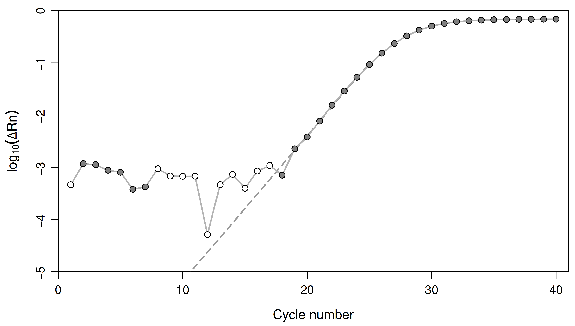
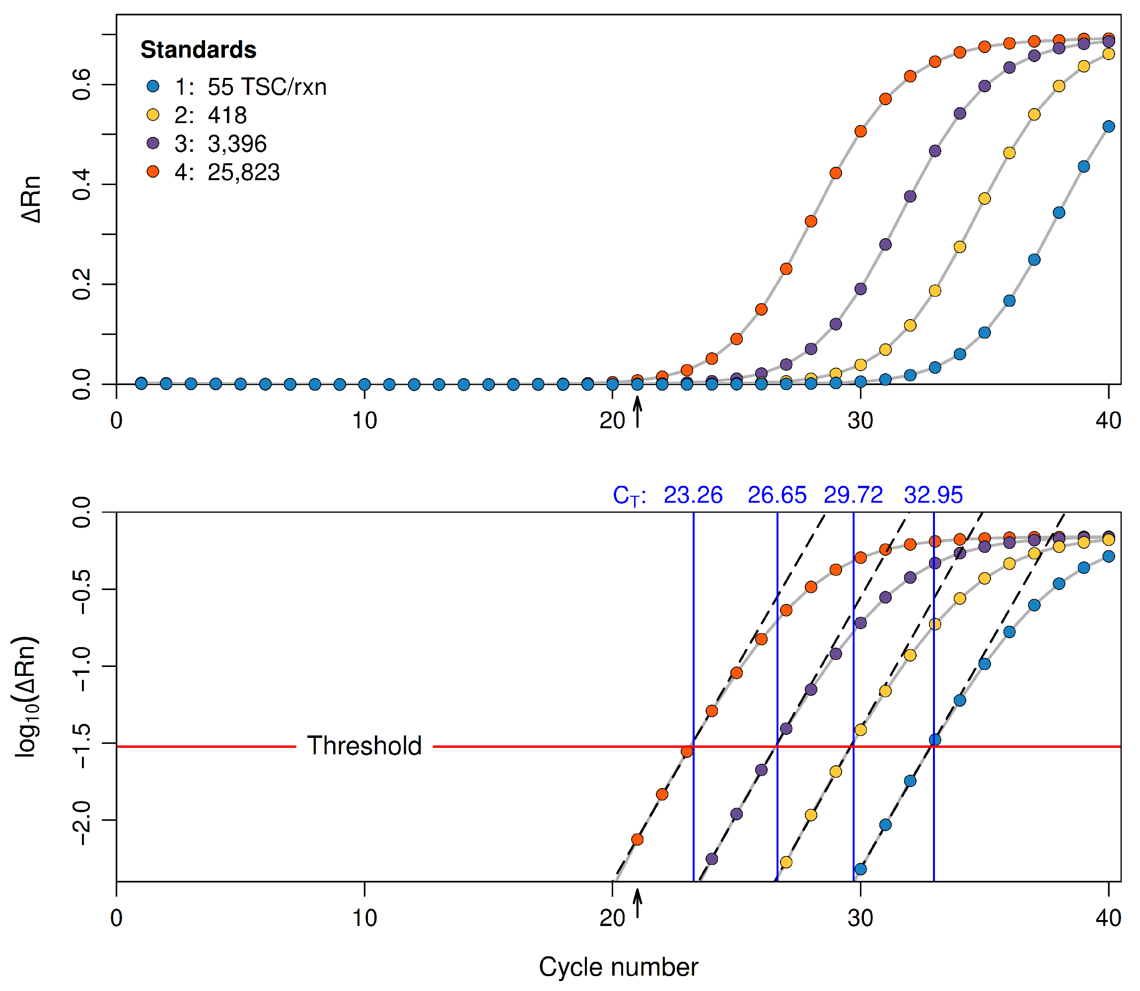
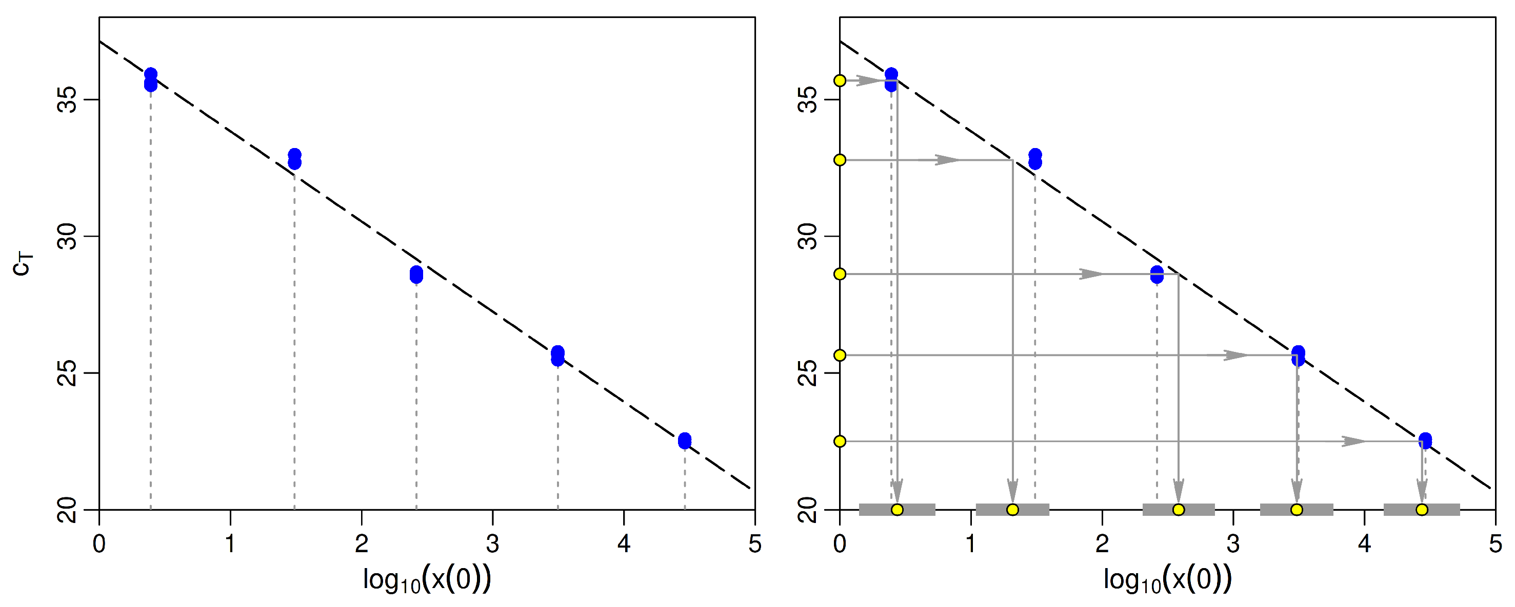
Appendix A. Example of a qPCR Workflow

To illustrate how qPCR is implemented in practice, we now outline the workflow for EPA Draft Method C [44,45,73]. This method is commonly used in the United States for estimating concentrations of the fecal indicator bacterium E. coli in recreational waterbodies when same-day results are desired. For the past nine years, our labs have used it with Applied Biosystems’ StepOnePlus® qPCR instruments (Thermo Fisher Scientific Inc., Waltham, Massachusetts, USA) to monitor E. coli levels at recreational beaches on various lakes and rivers in Michigan.
Prior to starting a qPCR run, all workspaces and pipets are thoroughly disinfected using UV light. All steps are performed using aseptic techniques to prevent contamination, and all preparatory work occurs on cold blocks.
After disinfecting surfaces, the assay mix containing all materials necessary for facilitating a polymerase chain reaction is prepared. The components consist of TaqMan master mix, bovine serum albumin (BSA), synthetic oligonucleotides (primers and probes), and certified nuclease-free water. The master mix contains thermostable DNA polymerase (Taq polymerase), deoxynucleotide triphosphate, and a reference dye, all suspended in a buffer for stability. This mix and the synthetic oligonucleotides facilitate the reaction in each sample. Typical concentrations of primers and probes in a qPCR reaction are 1000 nM for primers and 80 nM for probes. BSA is used as a stabilizer for the Taq polymerase enzyme and reduces the influence of inhibitors. Nuclease-free water is added to dilute the synthetic oligonucleotides to their appropriate concentrations. All of these components are thoroughly vortexed to form a homogeneous mixture and are added to a single tube. This tube is then vortexed, and an equal volume of the assay mix is added to each well of a multi-well plate, being careful to avoid creating droplets or air bubbles. Typical amounts are 20–23 μL of assay mix per well.
The next step is to add sample (or standard) and control solutions to the appropriate wells (methods of sample preparation are outlined above in Section 2.1). Typically, 2–5 μL of sample or control solution is added to the assay mix in each well, as required to yield a total volume of 25 μL. Every qPCR plate contains no-template controls consisting of nuclease-free water, a method blank that was run through the sample processing steps, and a positive control. In some cases, a standard curve (Section 2.3.2) is run with each plate to increase the accuracy of quantification.
After the assay mix, sample, and control solutions have been added to the wells, the qPCR plate is sealed and placed in a thermocycler, which monitors fluorescence in each well in real-time during a series of PCR amplification cycles. Software supplied with the thermocycler then determines the threshold cycle c T at which the appropriate measure of fluorescence ( log 10 ( Δ R n ) , Section 2.3.2) for each sample or standard first crossed the threshold. A typical run consists of 40 cycles and requires about 90 min.
Finally, a standard curve is fitted to data comprising pairs of known log 10 -transformed initial copy numbers for a series of standards (the “independent” variable, log 10 ( x 0 ) ) and corresponding measured c T values (the “dependent” variable), as discussed below in Section 2.4. Unknown log 10 -transformed copy numbers in the sample plus assay mix (S+AM) for environmental samples can then be estimated by inverting the fitted standard curve (so that c T becomes the independent variable and log 10 ( x 0 ) becomes the dependent variable, Section 2.3.3) and inserting the measured c T values for the samples. If desired, these copy numbers can be converted to concentrations in the S+AM, and can also be converted to concentrations in the original field samples by adjusting for all concentration and dilution steps during sample preparation and analysis.

Appendix B. Justification of an Approximation

Here, we justify the approximation by which we obtained Equation (18) from Equation (17) in the main text.
As noted in the main text, the definition of the threshold cycle implies that Δ R n ( c ) = τ when c = C T in Equation (14). That is, we require
φ ρ x 0 λ 1 = τ .
This equation can be rearranged to obtain
λ C T = τ ρ φ x 0 + 1 = τ ρ φ x 0 1 + φ x 0 τ ρ
Taking base-10 logarithms,
C T log 10 ( λ ) = log 10 τ ρ φ x 0 + log 10 1 + φ x 0 τ ρ .
From Equation (A2),
τ ρ φ x 0 = λ C T 1 , φ x 0 τ ρ = 1 λ C T 1 .
As pointed out in the main text, the cycle number at which Δ R n ( c ) crosses threshold τ typically ranges from roughly 20 to 35, and λ 2 . It follows that, in practice,
τ ρ φ x 0 > 10 6 , φ x 0 τ ρ < 10 6 .
Therefore,
log 10 τ ρ φ x 0 > 6 , log 10 1 + φ x 0 τ ρ log 10 ( e ) φ x 0 τ ρ < 10 6 .
All of which is to say that the second term on the right side of Equation (A3) is negligible in comparison with the first term on the right, so that, to a very good approximation,
C T log 10 ( λ ) = log 10 τ ρ φ x 0 .
A simple manipulation yields
C T = log 10 ( τ ρ / φ ) log 10 ( λ ) 1 log 10 ( λ ) · log 10 ( x 0 ) = β 0 + β 1 log 10 ( x 0 ) ,
which is Equation (18) of the main text.

Appendix C. Example of a ddPCR Workflow

We now provide a concrete example of a ddPCR workflow to illustrate how ddPCR is implemented in practice. The workflow we outline here was developed at Michigan State University [31] and has been used extensively in monitoring SARS-CoV-2 concentrations in wastewater samples across the state of Michigan. We have been using it for this purpose since 2019, with Bio-Rad’s QX200® ddPCR instruments (Bio-Rad Laboratories Inc., Hercules, CA, USA).
Similar to qPCR, all work surfaces are disinfected, all preparation is done using aseptic techniques, and all preparatory work occurs on cold blocks. The assay mix for ddPCR consists of supermix, synthetic oligonucleotides, and certified nuclease-free water. A key difference between supermix and master mix is that the supermix which normally is used contains no deoxynucleotide triphosphate. Typical concentrations for the oligonucleotides are 900 nM for the primers and 250 nM for the probe. Nuclease-free water is used to dilute the synthetic oligonucleotides to their appropriate concentration. All assay mix reagents are thoroughly vortexed to ensure a homogeneous solution, and the final combined mix is also vortexed before plating to ensure homogeneity. Each ddPCR reaction contains 16.5 μL of assay mix and 5.5 μL of sample or control. For quality control, every ddPCR run has a positive, negative, and no-template control. After the assay mix and samples/controls are plated, the plate is sealed with foil, vortexed to ensure homogeneity, and centrifuged to ensure all components are at the bottom of each reaction well. The plate is then placed in a droplet generator, where 20 μL of the S+AM is added to a generator cartridge.
Pressurized air pushes the S+AM and oil through separate microchannels which, as they merge, partition the S+AM into approximately 20,000 nanoliter-size droplets with a final volume (droplets in oil) of approximately 40 μL. This mixture of S+AM and oil is pipetted into a new plate. After all wells are filled in this way, the new plate is sealed with foil and placed on a thermocycler for amplification. When amplification is complete, the plate is placed on a droplet reader where a needle pierces each well, aspirates the contents, and passes the droplets through the droplet reader, where the fluorescence amplitude of droplets is measured, one droplet at a time. The analyst sets a fluorescence intensity threshold, which software for the droplet reader uses to classify droplets as positive (fluorescence intensity greater than the threshold) or negative (fluorescence intensity less than the threshold). The software then uses the number of negative droplets, the total number of droplets, and an assumed mean droplet volume to calculate the TSC concentration in the S+AM (Section 3.2.1).

Appendix D. Justification of an Upper Bound Based on Chebychev’s Inequality

Here, we derive the inequality in Equation (63) of the main text, using Chebychev’s inequality. Let X be a random variable with mean E ( X ) and finite variance V ( X ) > 0 . Then, for any δ > 0 , Chebychev’s inequality states that
P ( | X E ( X ) | > δ ) V ( X ) δ 2
e.g., [74] (p. 30). Now let
X = v ¯ m / μ v ,
where
v ¯ m = 1 m i = 1 m v i > 0 , μ v = E ( v i ) > 0 for all i .
We assume droplet volumes v i > 0 are independent identically distributed random variables with finite mean and variance. Then, E ( v ¯ m ) = μ v > 0 and
E ( X ) = 1 , V ( X ) = V ( v ¯ m ) μ v 2 = 1 m V ( v i ) μ v 2 = 1 m CV 2 ,
where CV denotes the coefficient of variation of droplet volume. It follows that
P ( | X E ( X ) | > δ ) = P v ¯ m μ v 1 > δ = P ( | v ¯ m μ v | / μ v > δ )
and
V ( X ) δ 2 = 1 m C V δ 2 .
Substituting these expressions for P ( | X E ( X ) | > δ ) and V ( X ) / δ 2 in Equation (A9) yields
P ( | v ¯ m μ v | / μ v > δ ) 1 m C V δ 2 ,
which is Equation (63) of the main text.

References

  1. Kleppe, K.; Ohtsuka, E.; Kleppe, R.; Molineux, I.; Khorana, H. Studies on polynucleotides: XCVI. Repair replication of short synthetic DNA’s as catalyzed by DNA polymerases. J. Mol. Biol. 1971, 56, 341–361. [Google Scholar] [CrossRef] [PubMed]
  2. Saiki, R.K.; Scharf, S.; Faloona, F.; Mullis, K.B.; Horn, G.T.; Erlich, H.A.; Arnheim, N. Enzymatic amplification of β-globin genomic sequences and restriction site analysis for diagnosis of sickle cell anemia. Science 1985, 230, 1350–1354. [Google Scholar] [CrossRef] [PubMed]
  3. Mullis, K.; Faloona, F.; Scharf, S.; Saiki, R.; Horn, G.; Erlich, H. Specific enzymatic amplification of DNA in vitro: The polymerase chain reaction. In Proceedings of the Cold Spring Harbor Symposia on Quantitative Biology; Cold Spring Harbor Laboratory Press: Cold Spring Harbor, NY, USA, 1986; Volume 51, pp. 263–273. [Google Scholar]
  4. Mullis, K.B.; Faloona, F.A. Specific synthesis of DNA in vitro via a polymerase-catalyzed chain reaction. In Methods in Enzymology; Elsevier: Amsterdam, The Netherlands, 1987; Volume 155, pp. 335–350. [Google Scholar]
  5. Shanks, O.C.; White, K.; Kelty, C.A.; Hayes, S.; Sivaganesan, M.; Jenkins, M.; Varma, M.; Haugland, R.A. Performance assessment PCR-based assays targeting Bacteroidales genetic markers of bovine fecal pollution. Appl. Environ. Microbiol. 2010, 76, 1359–1366. [Google Scholar] [CrossRef] [PubMed]
  6. Shanks, O.C.; Kelty, C.A.; Peed, L.; Sivaganesan, M.; Mooney, T.; Jenkins, M. Age-related shifts in the density and distribution of genetic marker water quality indicators in cow and calf feces. Appl. Environ. Microbiol. 2014, 80, 1588–1594. [Google Scholar] [CrossRef]
  7. USEPA. Recreational Water Quality Criteria; Technical Report 820-F-12-058; U.S. Environmental Protection Agency: Washington, DC, USA, 2012.
  8. Higuchi, R.; Fockler, C.; Dollinger, G.; Watson, R. Kinetic PCR analysis: Real-time monitoring of DNA amplification reactions. Bio/technology 1993, 11, 1026–1030. [Google Scholar] [CrossRef]
  9. Basu, A.S. Digital assays part I: Partitioning statistics and digital PCR. SLAS Technol. Transl. Life Sci. Innov. 2017, 22, 369–386. [Google Scholar] [CrossRef]
  10. Sykes, P.; Neoh, S.; Brisco, M.; Hughes, E.; Condon, J.; Morley, A. Quantitation of targets for PCR by use of limiting dilution. Biotechniques 1992, 13, 444–449. [Google Scholar]
  11. Vogelstein, B.; Kinzler, K.W. Digital PCR. Proc. Natl. Acad. Sci. USA 1999, 96, 9236–9241. [Google Scholar] [CrossRef]
  12. Burns, M.A.; Mastrangelo, C.H.; Sammarco, T.S.; Man, F.P.; Webster, J.R.; Johnsons, B.; Foerster, B.; Jones, D.; Fields, Y.; Kaiser, A.R.; et al. Microfabricated structures for integrated DNA analysis. Proc. Natl. Acad. Sci. USA 1996, 93, 5556–5561. [Google Scholar] [CrossRef]
  13. Burns, M.A.; Johnson, B.N.; Brahmasandra, S.N.; Handique, K.; Webster, J.R.; Krishnan, M.; Sammarco, T.S.; Man, P.M.; Jones, D.; Heldsinger, D.; et al. An integrated nanoliter DNA analysis device. Science 1998, 282, 484–487. [Google Scholar] [CrossRef]
  14. Ferrance, J.P.; Giordano, B.; Landers, J.P. Toward effective PCR-based amplification of DNA on microfabricated chips. In Capillary Electrophoresis of Nucleic Acids: Volume II: Practical Applications of Capillary Electrophoresis; Humana Press: Totowa, NJ, USA, 2001; pp. 191–204. [Google Scholar]
  15. Hindson, B.J.; Ness, K.D.; Masquelier, D.A.; Belgrader, P.; Heredia, N.J.; Makarewicz, A.J.; Bright, I.J.; Lucero, M.Y.; Hiddessen, A.L.; Legler, T.C.; et al. High-throughput droplet digital PCR system for absolute quantitation of DNA copy number. Anal. Chem. 2011, 83, 8604–8610. [Google Scholar] [CrossRef] [PubMed]
  16. Sekar, R.; Jin, X.; Liu, S.; Lu, J.; Shen, J.; Zhou, Y.; Gong, Z.; Feng, X.; Guo, S.; Li, W. Fecal contamination and high nutrient levels pollute the watersheds of Wujiang, China. Water 2021, 13, 457. [Google Scholar] [CrossRef]
  17. McNair, J.N.; Lane, M.J.; Hart, J.J.; Porter, A.M.; Briggs, S.; Southwell, B.; Sivy, T.; Szlag, D.C.; Scull, B.T.; Pike, S.; et al. Validity assessment of Michigan’s proposed qPCR threshold value for rapid water-quality monitoring of E. coli contamination. Water Res. 2022, 226, 119235. [Google Scholar] [CrossRef] [PubMed]
  18. McNair, J.N.; Rediske, R.R.; Hart, J.J.; Jamison, M.N.; Briggs, S. Performance of Colilert-18 and qPCR for monitoring E. coli contamination at freshwater beaches in Michigan. Environments 2025, 12, 21. [Google Scholar] [CrossRef]
  19. Ballesté, E.; Demeter, K.; Masterson, B.; Timoneda, N.; Sala-Comorera, L.; Meijer, W.G. Implementation and integration of microbial source tracking in a river watershed monitoring plan. Sci. Total Environ. 2020, 736, 139573. [Google Scholar] [CrossRef]
  20. Cao, Y.; Raith, M.R.; Griffith, J.F. Droplet digital PCR for simultaneous quantification of general and human-associated fecal indicators for water quality assessment. Water Res. 2015, 70, 337–349. [Google Scholar] [CrossRef]
  21. Frick, C.; Vierheilig, J.; Nadiotis-Tsaka, T.; Ixenmaier, S.; Linke, R.; Reischer, G.H.; Komma, J.; Kirschner, A.K.; Mach, R.L.; Savio, D.; et al. Elucidating fecal pollution patterns in alluvial water resources by linking standard fecal indicator bacteria to river connectivity and genetic microbial source tracking. Water Res. 2020, 184, 116132. [Google Scholar] [CrossRef]
  22. Flood, M.T.; Hernandez-Suarez, J.S.; Nejadhashemi, A.P.; Martin, S.L.; Hyndman, D.; Rose, J.B. Connecting microbial, nutrient, physiochemical, and land use variables for the evaluation of water quality within mixed use watersheds. Water Res. 2022, 219, 118526. [Google Scholar] [CrossRef]
  23. Hart, J.J.; Jamison, M.N.; McNair, J.N.; Woznicki, S.A.; Jordan, B.; Rediske, R.R. Using watershed characteristics to enhance fecal source identification. J. Environ. Manag. 2023, 336, 117642. [Google Scholar] [CrossRef]
  24. Jamison, M.N.; Hart, J.J.; Szlag, D.C. Improving the identification of fecal contamination in recreational water through the standardization and normalization of microbial source tracking. Environ. Sci. Technol. Water 2022, 2, 2305–2311. [Google Scholar] [CrossRef]
  25. Pendergraph, D.P.; Ranieri, J.; Ermatinger, L.; Baumann, A.; Metcalf, A.L.; DeLuca, T.H.; Church, M.J. Differentiating sources of fecal contamination to wilderness waters using droplet digital PCR and fecal indicator bacteria methods. Wilderness Environ. Med. 2021, 32, 332–339. [Google Scholar] [CrossRef] [PubMed]
  26. Shrestha, A.; Kelty, C.A.; Sivaganesan, M.; Shanks, O.C.; Dorevitch, S. Fecal pollution source characterization at non-point source impacted beaches under dry and wet weather conditions. Water Res. 2020, 182, 116014. [Google Scholar] [CrossRef] [PubMed]
  27. Steinbacher, S.; Savio, D.F.; Demeter, K.; Karl, M.; Kandler, W.; Kirschner, A.K.; Reischer, G.H.; Ixenmaier, S.K.; Mayer, R.; Mach, R.L.; et al. Genetic microbial faecal source tracking: Rising technology to support future water quality testing and safety management. Österreichische Wasser-Abfallwirtsch. 2021, 73, 468–481. [Google Scholar] [CrossRef]
  28. Doi, H.; Takahara, T.; Minamoto, T.; Matsuhashi, S.; Uchii, K.; Yamanaka, H. Droplet digital polymerase chain reaction (PCR) outperforms real-time PCR in the detection of environmental DNA from an invasive fish species. Environ. Sci. Technol. 2015, 49, 5601–5608. [Google Scholar] [CrossRef]
  29. Doi, H.; Uchii, K.; Takahara, T.; Matsuhashi, S.; Yamanaka, H.; Minamoto, T. Use of droplet digital PCR for estimation of fish abundance and biomass in environmental DNA surveys. PLoS ONE 2015, 10, e0122763. [Google Scholar] [CrossRef]
  30. Te, S.H.; Chen, E.Y.; Gin, K.Y.H. Comparison of quantitative PCR and droplet digital PCR multiplex assays for two genera of bloom-forming cyanobacteria, Cylindrospermopsis and Microcystis. Appl. Environ. Microbiol. 2015, 81, 5203–5211. [Google Scholar] [CrossRef]
  31. Flood, M.T.; D’Souza, N.; Rose, J.B.; Aw, T.G. Methods evaluation for rapid concentration and quantification of SARS-CoV-2 in raw wastewater using droplet digital and quantitative RT-PCR. Food Environ. Virol. 2021, 13, 303–315. [Google Scholar] [CrossRef]
  32. Schmitz, B.W.; Innes, G.K.; Prasek, S.M.; Betancourt, W.Q.; Stark, E.R.; Foster, A.R.; Abraham, A.G.; Gerba, C.P.; Pepper, I.L. Enumerating asymptomatic COVID-19 cases and estimating SARS-CoV-2 fecal shedding rates via wastewater-based epidemiology. Sci. Total Environ. 2021, 801, 149794. [Google Scholar] [CrossRef]
  33. Wu, J.; Wang, Z.; Lin, Y.; Zhang, L.; Chen, J.; Li, P.; Liu, W.; Wang, Y.; Yao, C.; Yang, K. Technical framework for wastewater-based epidemiology of SARS-CoV-2. Sci. Total Environ. 2021, 791, 148271. [Google Scholar] [CrossRef]
  34. Ciesielski, M.; Blackwood, D.; Clerkin, T.; Gonzalez, R.; Thompson, H.; Larson, A.; Noble, R. Assessing sensitivity and reproducibility of RT-ddPCR and RT-qPCR for the quantification of SARS-CoV-2 in wastewater. J. Virol. Methods 2021, 297, 114230. [Google Scholar] [CrossRef]
  35. Hart, J.J.; Jamison, M.N.; McNair, J.N.; Szlag, D.C. Frequency and degradation of SARS-CoV-2 markers N1, N2, and E in sewage. J. Water Health 2023, 21, 514–524. [Google Scholar] [CrossRef] [PubMed]
  36. Raeymaekers, L. Basic principles of quantitative PCR. Mol. Biotechnol. 2000, 15, 115–122. [Google Scholar] [CrossRef] [PubMed]
  37. Rutledge, R.; Cote, C. Mathematics of quantitative kinetic PCR and the application of standard curves. Nucleic Acids Res. 2003, 31, e93. [Google Scholar] [CrossRef] [PubMed]
  38. Stephenson, F.H. Calculations for Molecular Biology and Biotechnology; Academic Press: New York, NY, USA, 2016. [Google Scholar]
  39. Thermo-Fisher. Real-Time PCR Handbook; Technical report; Thermo Fisher Scientific Inc.: Waltham, MA, USA, 2016. [Google Scholar]
  40. Bio-Rad. Droplet Digital PCR Applications Guide; Technical Report Bulletin 6407 B; Bio-Rad Laboratories, Inc.: Hercules, CA, USA, 2018. [Google Scholar]
  41. Vadde, K.K.; Moghadam, S.V.; Jafarzadeh, A.; Matta, A.; Phan, D.C.; Johnson, D.; Kapoor, V. Precipitation impacts the physicochemical water quality and abundance of microbial source tracking markers in urban Texas watersheds. PLoS Water 2024, 3, e0000209. [Google Scholar] [CrossRef]
  42. Kaltenboeck, B.; Wang, C. Advances in real-time PCR: Application to clinical laboratory diagnostics. Adv. Clin. Chem. 2005, 40, 219. [Google Scholar]
  43. Arya, M.; Shergill, I.S.; Williamson, M.; Gommersall, L.; Arya, N.; Patel, H.R. Basic principles of real-time quantitative PCR. Expert Rev. Mol. Diagn. 2005, 5, 209–219. [Google Scholar] [CrossRef]
  44. Aw, T.G.; Sivaganesan, M.; Briggs, S.; Dreelin, E.; Aslan, A.; Dorevitch, S.; Shrestha, A.; Isaacs, N.; Kinzelman, J.; Kleinheinz, G.; et al. Evaluation of multiple laboratory performance and variability in analysis of recreational freshwaters by a rapid Escherichia coli qPCR method (Draft Method C). Water Res. 2019, 156, 465–474. [Google Scholar] [CrossRef]
  45. Sivaganesan, M.; Aw, T.G.; Briggs, S.; Dreelin, E.; Aslan, A.; Dorevitch, S.; Shrestha, A.; Isaacs, N.; Kinzelman, J.; Kleinheinz, G.; et al. Standardized data quality acceptance criteria for a rapid Escherichia coli qPCR method (Draft Method C) for water quality monitoring at recreational beaches. Water Res. 2019, 156, 456–464. [Google Scholar] [CrossRef]
  46. Thermo-Fisher. Application Note: Understanding Ct; Technical report; Thermo Fisher Scientific Inc.: Waltham, MA, USA, 2016. [Google Scholar]
  47. Thermo-Fisher. Application Note: ROX Passive Reference Dye for Troubleshooting Real-Time PCR; Technical report; Thermo Fisher Scientific Inc.: Waltham, MA, USA, 2015. [Google Scholar]
  48. Bio-Rad. Real-Time PCR Applications Guide; Technical Report Bulletin 5279; Bio-Rad Laboratories, Inc.: Hercules, CA, USA, 2006. [Google Scholar]
  49. Parker, P.A.; Vining, G.G.; Wilson, S.R.; Szarka, J.L., III; Johnson, N.G. The prediction properties of classical and inverse regression for the simple linear calibration problem. J. Qual. Technol. 2010, 42, 332–347. [Google Scholar] [CrossRef]
  50. Nappier, S.P.; Ichida, A.; Jaglo, K.; Haugland, R.; Jones, K.R. Advancements in mitigating interference in quantitative polymerase chain reaction (qPCR) for microbial water quality monitoring. Sci. Total Environ. 2019, 671, 732–740. [Google Scholar] [CrossRef]
  51. Sidstedt, M.; Rådström, P.; Hedman, J. PCR inhibition in qPCR, dPCR and MPS—Mechanisms and solutions. Anal. Bioanal. Chem. 2020, 412, 2009–2023. [Google Scholar] [CrossRef] [PubMed]
  52. Sivaganesan, M.; Varma, M.; Siefring, S.; Haugland, R. Quantification of plasmid DNA standards for US EPA fecal indicator bacteria qPCR methods by droplet digital PCR analysis. J. Microbiol. Methods 2018, 152, 135–142. [Google Scholar] [CrossRef] [PubMed]
  53. Corbisier, P.; Pinheiro, L.; Mazoua, S.; Kortekaas, A.M.; Chung, P.Y.J.; Gerganova, T.; Roebben, G.; Emons, H.; Emslie, K. DNA copy number concentration measured by digital and droplet digital quantitative PCR using certified reference materials. Anal. Bioanal. Chem. 2015, 407, 1831–1840. [Google Scholar] [CrossRef]
  54. Dagata, J.A.; Farkas, N.; Kramer, J. Method for measuring the volume of nominally 100 μm diameter spherical water-in-oil emulsion droplets. NIST Spec. Publ. 2016, 260, 260-184. [Google Scholar]
  55. Košir, A.B.; Divieto, C.; Pavšič, J.; Pavarelli, S.; Dobnik, D.; Dreo, T.; Bellotti, R.; Sassi, M.P.; Žel, J. Droplet volume variability as a critical factor for accuracy of absolute quantification using droplet digital PCR. Anal. Bioanal. Chem. 2017, 409, 6689–6697. [Google Scholar] [CrossRef] [PubMed]
  56. Ryan, T. Modern Regression Methods; John Wiley & Sons, Inc.: Hoboken, NJ, USA, 1997. [Google Scholar]
  57. R Core Team. R: A Language and Environment for Statistical Computing; R Foundation for Statistical Computing: Vienna, Austria, 2024. [Google Scholar]
  58. Kokkoris, V.; Vukicevich, E.; Richards, A.; Thomsen, C.; Hart, M.M. Challenges using droplet digital PCR for environmental samples. Appl. Microbiol. 2021, 1, 74–88. [Google Scholar] [CrossRef]
  59. Pinheiro, L.B.; Coleman, V.A.; Hindson, C.M.; Herrmann, J.; Hindson, B.J.; Bhat, S.; Emslie, K.R. Evaluation of a droplet digital polymerase chain reaction format for DNA copy number quantification. Anal. Chem. 2012, 84, 1003–1011. [Google Scholar] [CrossRef]
  60. Balakrishnan, N.; Nevzorov, V.B. A Primer on Statistical Distributions; John Wiley & Sons: Hoboken, NJ, USA, 2003. [Google Scholar]
  61. Forbes, C.; Evans, M.; Hastings, N.; Peacock, B. Statistical Distributions; John Wiley & Sons: Hoboken, NJ, USA, 2011. [Google Scholar]
  62. Brown, L.D.; Cai, T.T.; DasGupta, A. Interval estimation for a binomial proportion. Stat. Sci. 2001, 16, 101–133. [Google Scholar] [CrossRef]
  63. Agresti, A.; Coull, B.A. Approximate is better than “exact” for interval estimation of binomial proportions. Am. Stat. 1998, 52, 119–126. [Google Scholar]
  64. Efron, B.; Tibshirani, R.J. An Introduction to the Bootstrap; Chapman and Hall/CRC: New York, NY, USA, 1994. [Google Scholar]
  65. Dorai-Raj, S. binom: Binomial Confidence Intervals for Several Parameterizations; R Package Version 1.1-1.1. 2022. [Google Scholar]
  66. Canty, A.; Ripley, B. boot: Bootstrap R (S-Plus) Functions; R Package Version 1.1-1.1. 2024. [Google Scholar]
  67. Tibshirani, R.; Leisch, F. bootstrap: Functions for the Book “An Introduction to the Bootstrap”; R Package Version 2019.6. 2019. [Google Scholar]
  68. Dingle, T.C.; Sedlak, R.H.; Cook, L.; Jerome, K.R. Tolerance of droplet-digital PCR vs real-time quantitative PCR to inhibitory substances. Clin. Chem. 2013, 59, 1670–1672. [Google Scholar] [CrossRef]
  69. Verhaegen, B.; De Reu, K.; De Zutter, L.; Verstraete, K.; Heyndrickx, M.; Van Coillie, E. Comparison of droplet digital PCR and qPCR for the quantification of Shiga toxin-producing Escherichia coli in bovine feces. Toxins 2016, 8, 157. [Google Scholar] [CrossRef] [PubMed]
  70. Sze, M.A.; Abbasi, M.; Hogg, J.C.; Sin, D.D. A comparison between droplet digital and quantitative PCR in the analysis of bacterial 16S load in lung tissue samples from control and COPD GOLD 2. PLoS ONE 2014, 9, e110351. [Google Scholar] [CrossRef] [PubMed]
  71. Choi, C.H.; Kim, E.; Yang, S.M.; Kim, D.S.; Suh, S.M.; Lee, G.Y.; Kim, H.Y. Comparison of real-time PCR and droplet digital PCR for the quantitative detection of Lactiplantibacillus plantarum subsp. plantarum. Foods 2022, 11, 1331. [Google Scholar] [CrossRef]
  72. Chandler, D. Redefining relativity: Quantitative PCR at low template concentrations for industrial and environmental microbiology. J. Ind. Microbiol. Biotechnol. 1998, 21, 128–140. [Google Scholar] [CrossRef]
  73. Lane, M.J.; McNair, J.N.; Rediske, R.R.; Briggs, S.; Sivaganesan, M.; Haugland, R. Simplified analysis of measurement data from a rapid E. coli qPCR method (EPA Draft Method C) using a standardized Excel workbook. Water 2020, 12, 775. [Google Scholar] [CrossRef] [PubMed]
  74. Çinlar, E. Introduction to Stochastic Processes; Dover Publications, Inc.: Mineola, NY, USA, 2013. [Google Scholar]
Figure 1. An individual amplification curve for an E. coli target sequence standard with 25,823 copies per reaction. Points represent background-corrected normalized reporter fluorescence ( Δ R n , Section 2.3.1) in an individual plate well during successive PCR cycles, plotted on a log 10 scale. Transformed values begin to increase roughly linearly at cycle 19 (indicating geometric increase), with approximate linearity extending to cycle 25. For cycles prior to cycle 19, fluorescence due to free reporters is well below background, leaving only random measurement error after correction. Because background correction is not exact, several of the Δ R n values prior to cycle 19 were negative. These values were incremented by 0.0011 to permit log 10 transformation, then plotted as white-filled circles; unadjusted values are plotted as red-filled circles. The dashed line represents fluorescence due to free reporters that would be seen at early cycles of geometric increase if background correction were exact and the low background-corrected fluorescence levels were measurable. Data: Molly J. Lane, Robert B. Annis Water Resources Institute.
Water 17 00381 g001
Figure 2. Amplification curves for a series of four E. coli target sequence standards with known numbers of target sequence copies per reaction (TSC/rxn). Points are averages of three replicates per standard. Standard concentrations increase from right to left and are plotted with different colors. (Top) Background-corrected normalized reporter fluorescence Δ R n (a measure of fluorescence reported by the analytical instrument, Section 2.3.1) versus PCR cycle number. (Bottom) Log10 background-corrected normalized reporter fluorescence log 10 ( Δ R n ) versus cycle number. Dashed black lines are linear regression models fitted to the linear portion of each Δ R n curve. The red horizontal line passing through the linear portions of these curves is the fluorescence threshold; the fractional cycle numbers at which the Δ R n ( c ) curves intersect this threshold are indicated by vertical blue lines and are the corresponding threshold cycles c T (blue numbers at the top of the panel), which are discussed in Section 2.3.2. The arrow on the horizontal axis in the top panel indicates the lowest cycle number for which data are included in the bottom panel. Data: Molly J. Lane, Robert B. Annis Water Resources Institute; data for standard 4 were used to create Figure 1.
Water 17 00381 g002
Figure 3. The main steps in target sequence amplification and the corresponding production of fluorescing free reporters with qPCR. (Top) Schematic diagram of the main steps within a single amplification cycle of a target DNA sequence, which comprise denaturation of DNA at 95 °C, annealing of forward and reverse primers and probe at 50 °C, and primer extension and probe cleavage at 72 °C. (Middle) Schematic diagram of four amplification cycles of a target sequence, including production of fluorescing free reporters. D: denaturation; A: annealing; E: extension. (Bottom) Summary of the cumulative numbers of DAE cycles, target sequence copies, and fluorescing free reporters produced in the four amplification cycles shown in the middle panel for the ideal case where amplification efficiency is 100%.
Water 17 00381 g003
Figure 4. Example of the relationship between measured c T values (blue dots) and log 10 ( x 0 ) in standards for a qPCR calibration run employing five standards with three replicates each. The dashed line is the fitted standard curve (linear regression model). Dotted vertical lines indicate log 10 ( x 0 ) values in standards. Left: Data and standard curve only. Standard concentrations are 2.5, 30.8, 261.3, 3125.3, and 29,066.7 gene copies per reaction. Right: Data and standard curve supplemented with five new c T values (yellow-filled dots on the vertical axis) and corresponding predicted log 10 ( x 0 ) values (yellow-filled dots on the horizontal axis) calculated with Equation (22). Arrows indicate direction of prediction. Also shown are estimated 95% confidence intervals (gray bars on the horizontal axis) for the predicted log 10 ( x 0 ) values. Numerical values of estimates are shown in Table 2. Data: John J. Hart, Robert B. Annis Water Resources Institute.
Water 17 00381 g004
Figure 5. Calibration results for a composite data set that includes data from six qPCR calibration runs, each with three replicates of the same five standards (total replicates per standard = 18). Standard concentrations are the same as in Figure 4. Three regression models were assessed and are listed at the top of the figure. Row 1: Data and fitted standard curves, with estimates of the intercept, slope, and mean absolute error (MAE). Row 2: Plots of regression residuals versus log 10 ( x 0 ) . Residuals for WLS models are those for the equivalent two-predictor model in Equation (36), since this is the model used to estimate parameter values and confidence intervals. Standard deviations of the residuals for each standard are listed at the bottom of the panel. Row 3: Box plots of regression residuals versus log 10 ( x 0 ) . P-values for Levene’s test are also shown. Row 4: Normal quantile–quantile plots of residuals, with 95% confidence envelopes. P-values for the Shapiro–Wilk test are also shown. Row 5: Inverse prediction of log 10 initial copy numbers of the five standards (filled yellow circles on the horizontal axis), based on means of the corresponding measured c T values (filled yellow circles on the vertical axis). Dotted vertical lines: actual log 10 initial copy numbers of the standards. Data: John J. Hart, Robert B. Annis Water Resources Institute.
Water 17 00381 g005
Figure 6. Schematic diagram of the process of droplet formation by a droplet generator as oil and S+AM flow through converging microchannels in a chip. Arrows in microchannels indicate direction of flow. Black dots represent TSC in the S+AM and are not drawn to scale. Average droplet diameter varies with experimental conditions but, typically, is on the order of 100 μm [53,54,55].
Water 17 00381 g006
Figure 7. Simplified example to illustrate how the multinomial distribution arises from partitioning the S+AM into droplets, with random allocation of TSC to droplets. In this simple case, there are only N = 5 TSC (black dots) and n = 6 droplets (blue disks). Each TSC has probability π j of being allocated to droplet j. Stars indicate droplets that, after amplification, will fluoresce in the droplet reader.
Water 17 00381 g007
Figure 8. Fluorescence amplitude (peak minus baseline) of individual droplets versus droplet or event number for three sample wells (C03, D03, and E03) containing replicates of an HF183 positive control. The horizontal magenta line at 429 on the vertical axis is the threshold fluorescence level; droplets fluorescing above this level are classified as positive for the HF183 marker (blue dots), and droplets below it as negative (gray dots). Results for different wells are separated by dashed vertical lines. The original figure was exported from Bio-Rad QuantaSoft software and enhanced to increase contrast. Data: John J. Hart, Robert B. Annis Water Resources Institute.
Water 17 00381 g008
Table 1. Symbols used in the qPCR equations. J: luminous intensity; –: dimensionless; DAE: denaturation, annealing, and extension; TSC: target sequence copies; S+AM: sample plus assay mix; WLS: weighted least-squares.
SymbolDimensionMeaning
ε Proportional amplification efficiency, 0 < ε 1
λ Amplification factor, λ = 1 + ε ( 1 , 2 ]
φ JFluorescence intensity per free reporter
κ w Well effect factor
B w JBackground fluorescence intensity
ρ JPassive dye fluorescence intensity
τ Threshold level of Δ R n
cDAE cycle number
c T Threshold cycle number
x ( c ) Number of TSC per reaction at the end of cycle c
x 0 Initial number x ( 0 ) of TSC per reaction, x 0 1
r ( c ) Number of free reporters per reaction
f ( c ) JNotional S+AM fluorescence with no background or well effect
g w ( c ) JNotional S+AM fluorescence with background but no well effect
R w ( c ) JMeasured S+AM fluorescence with background and well effect
P w JMeasured reference dye fluorescence with well effect
R n w ( c ) Normalized S+AM fluorescence with well effect removed
Δ R n ( c ) – *Normalized S+AM fluorescence with background and well effects removed
Y i Random variable representing the value of c T in sample i
y i Measured value of c T in sample i
β 0 c T intercept of a linear standard curve
β 1 Slope of a linear standard curve
ξ i Random error in the measured value of c T in sample i
u i Log10-transformed value of x 0 in sample i
w i Weight applied to the residual for sample i in WLS regression
Q ( β 0 , β 1 ) Sum of squared residuals, with or without weighting
Y ˜ i Re-scaled random variable Y ˜ i = Y i w i in WLS regression
y ˜ i Re-scaled measured value y ˜ i = y i w i in WLS regression
u ˜ i Re-scaled measured value u ˜ i = u i w i in WLS regression.
Note: * Dimensionless but sometimes reported in “relative fluorescence units” (RFU).
Table 2. Predicted values of log 10 ( x 0 ) and corresponding 95% confidence intervals for the five new c T values in Figure 4. LCL, UCL: 95% lower and upper confidence limits. Standard: log 10 initial copy numbers log 10 ( x 0 ) for the five standards in Figure 4.
New c T Predicted log 10 ( x 0 ) 95% LCL95% UCLStandard
35.690.440.150.730.39
32.791.321.041.601.49
28.622.582.312.862.42
25.653.483.203.763.49
22.504.444.154.734.46
Table 3. Symbols used in the ddPCR equations. L: length, –: dimensionless, S+AM: sample plus assay mix.
SymbolDimensionMeaning
v j L3Volume of droplet j
v ¯ L3Average droplet volume
VL3S+AM volume
nNumber of droplets
NNumber of TSC
π j Probability that any given TSC in S+AM is allocated to droplet j
π ¯ Average of π j over all droplets
Z j Random variable representing number of TSC allocated to droplet j
z j Realized number of TSC allocated to droplet j
P 0 Probability that any given droplet contains no TSC
mTotal number of droplets counted by the droplet reader
m 0 Number of negative droplets counted by the droplet reader
CL−3Estimated number of TSC per unit volume of S+AM.
Table 4. Counts of negative and all droplets m 0 and m, the resulting estimates of binomial probability P 0 and HF183 marker concentration C in S+AM (GC/μL), three types of 95% confidence interval (CI) for P 0 , and six types of 95% confidence interval for TSC concentration C S + AM (GC/μL) for the data plotted in Figure 8. “(boot)” indicates bootstrap methods. CI type “QuantaSoft” refers to the 95% confidence limits reported by Bio-Rad QuantaSoft software. For purposes of illustration, an estimated mean droplet volume of v ¯ = 0.85 nL = 8.5 × 10 4 μL, supplied by the instrument manufacturer, was used in calculations. LCL, UCL: lower and upper 95% confidence limits.
Well m 0 m P 0 CCI Type P 0 LCL P 0 UCLC LCLC UCL
C0316,56317,0730.9701335.7Wilson0.967470.9725832.738.9
Agresti–Coull0.967460.9725832.738.9
Wald0.967570.9726832.638.8
Percentile (boot)32.738.7
BC a (boot)32.838.9
QuantaSoft34.138.8
D0316,07216,5130.9732931.8Wilson0.970720.9756429.035.0
Agresti–Coull0.970720.9756529.035.0
Wald0.970830.9757528.934.8
Percentile (boot)28.834.9
BC a (boot)28.834.9
QuantaSoft30.334.8
E0316,32516,8090.9712134.4Wilson0.968570.9736331.437.6
Agresti–Coull0.968570.9736331.437.6
Wald0.968680.9737331.337.4
Percentile (boot)31.337.4
BC a (boot)31.337.9
QuantaSoft32.837.4
Table 5. Comparison of qPCR and ddPCR with respect to several factors that merit consideration when choosing between these methods for a particular application.
PropertyFactorqPCRddPCR
CostInstrumentation costLowerHigher
Per-sample costLowerHigher
Sample turnaround timeSample preparation and analysis timeShorterLonger
CalibrationStandard curve required?YesNo
Other calibration required or advisable?YesYes
InhibitionSensitivity to PCR inhibitionHigherLower
Limits of quantificationUpper limit of quantificationHigherLower
Lower limit of quantificationHigherLower
Dynamic rangeWiderNarrower
SimplicitySimplicity of laboratory analysisHigherLower
Simplicity of proper data analysisLowerHigher
Simplicity of the underlying theoryLowerHigher
Disclaimer/Publisher’s Note: The statements, opinions and data contained in all publications are solely those of the individual author(s) and contributor(s) and not of MDPI and/or the editor(s). MDPI and/or the editor(s) disclaim responsibility for any injury to people or property resulting from any ideas, methods, instructions or products referred to in the content.

