
A Case Study of the Debris Flows Event in the Chalk Cliffs Basin, Colorado, USA: Numerical Simulations Based on a Multi-Phase Flow Model

Abstract
1. Introduction
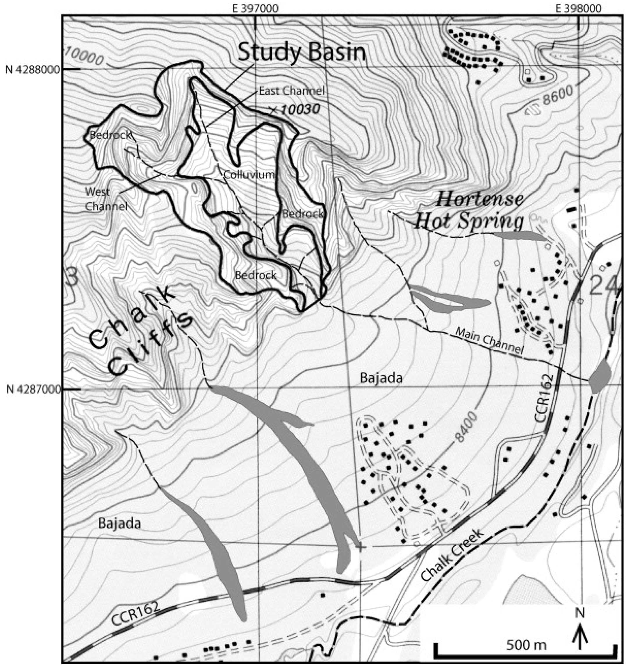
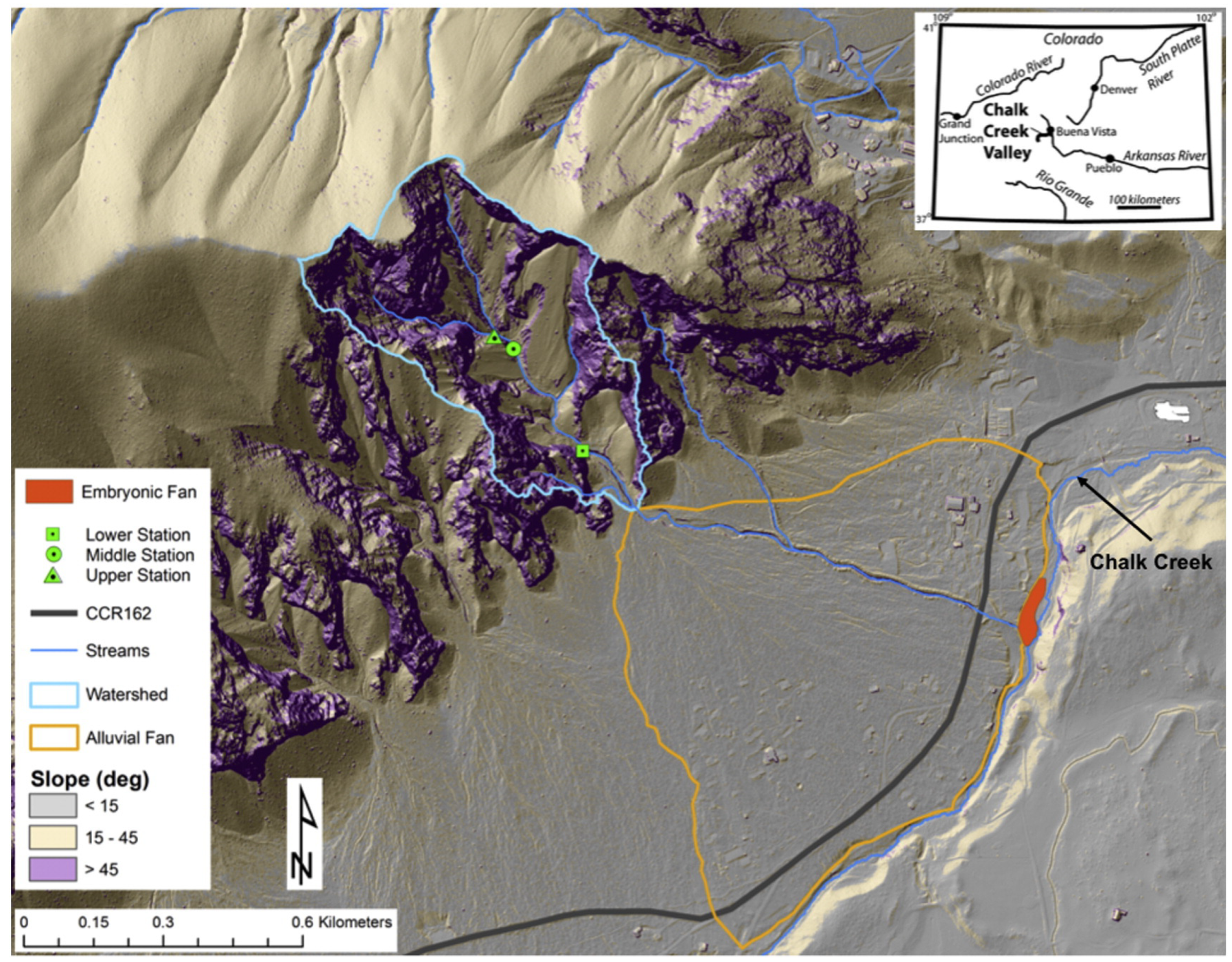
2. Study Area
3. Method
3.1. The Studied Debris Flow Event
3.2. Input Parameters
3.3. Sensitivity Analysis
4. Results
4.1. Analysis of the 15 September 2009 Event
4.2. Sensitivity Analysis
5. Discussion
6. Concluding Remarks
Author Contributions
Funding
Data Availability Statement
Conflicts of Interest
References
- Costa, J.E. Physical geomorphology of debris flows. In Developments and Applications of Geomorphology; Springer: Berlin/Heidelberg, Germany, 1984; pp. 268–317. [Google Scholar]
- Iverson, R.M.; Denlinger, R.P. The physics of debris flows—A conceptual assessment. In Proceedings of the International Symposium on Erosion and Sedimentation in the Pacific Rim, Corvallis, OR, USA, 3–7 August 1987; p. 165. [Google Scholar]
- Iverson, R.M. The physics of debris flows. Rev. Geophys. 1997, 35, 245–296. [Google Scholar] [CrossRef]
- Bozhinskiy, A.N.; Nazarov, A.N. Two-phase model of debris-flow. In Proceedings of the 2nd International Conference on Debris-Flow Hazards Mitigation: Mechanics, Prediction, and Assessment, Taipei, Taiwan, 16–18 August 2000; pp. 263–269. [Google Scholar]
- Coussot, P. Mudflow rheology and dynamics. In Mudflow Rheology and Dynamics; A.A. Balkema: Rotterdam, The Netherlands, 1997. [Google Scholar]
- Julien, P.; Leon, C. Mud floods, mudflows and debris flows. Classification, rheology and structural design. Jornadas Investig. JIFI 2000, 33, 1–15. [Google Scholar]
- Takahashi, T. Debris Flow: Mechanics, Prediction and Countermeasures; Taylor & Francis: London, UK, 2007. [Google Scholar]
- Iverson, R.M. Debris-flow mechanics. In Debris-flow Hazards and Related Phenomena; Springer: Berlin/Heidelberg, Germany, 2007; pp. 105–134. [Google Scholar]
- Trujillo-Vela, M.G.; Ramos-Canon, A.M.; Escobar-Vargas, J.A.; Galindo-Torres, S.A. An overview of debris-flow mathematical modelling. Earth Sci. Rev. 2022, 232, 104135. [Google Scholar] [CrossRef]
- Bagnold, R.A. Experiments on a gravity-free dispersion of large solid spheres in a Newtonian fluid under shear. Proc. R. Soc. Lond. Ser. Math. Phys. Sci. 1954, 225, 49–63. [Google Scholar]
- Johnson, A.M. Physical Processes in Geology: A Method for Interpretation of Natural Physical Processes in Geology Phenomena; Freeman Cooper: San Francisco, CA, USA, 1970. [Google Scholar]
- Takahashi, T. Debris Flow. Annu. Rev. Fluid Mech. 1981, 13, 57–77. [Google Scholar] [CrossRef]
- Davies, T.R.H. Large debris flows: A macro-viscous phenomenon. Acta Mech. 1986, 63, 161–178. [Google Scholar] [CrossRef]
- Chen, C. Generalized viscoplastic modeling of debris flow. J. Hydraul. Eng. 1988, 114, 237–258. [Google Scholar] [CrossRef]
- Pitman, E.B.; Le, L. A two-fluid model for avalanche and debris flows. Philos. Trans. R. Soc. Math. Phys. Eng. Sci. 2005, 363, 1573–1601. [Google Scholar] [CrossRef]
- Mousavi Tayebi, S.A.; Moussavi Tayyebi, S.; Pastor, M. Depth-Integrated Two-Phase Modeling of Two Real Cases: A Comparison between r.avaflow and GeoFlow-SPH Codes. Appl. Sci. 2021, 11, 5751. [Google Scholar] [CrossRef]
- Zhang, X.; Tang, C.; Yu, Y.; Tang, C.; Li, N.; Xiong, J.; Chen, M. Some Considerations for Using Numerical Methods to Simulate Possible Debris Flows: The Case of the 2013 and 2020 Wayao Debris Flows (Sichuan, China). Water 2022, 14, 1050. [Google Scholar] [CrossRef]
- KC, D.; Naqvi, M.W.; Hu, L. A Case Study and Numerical Modeling of Post-Wildfire Debris Flows in Montecito, California. Water 2024, 16, 1285. [Google Scholar] [CrossRef]
- Abraham, M.T.; Satyam, N.; Kowalski, J. Numerical Modelling of Debris Flows for Simulation-Based Decision Support: An Indian Perspective. Indian Geotech. J. 2024. [Google Scholar] [CrossRef]
- Pudasaini, S.P.; Fischer, J.T. A mechanical erosion model for two-phase mass flows. Int. J. Multiphase Flow 2020, 132, 103416. [Google Scholar] [CrossRef]
- Somos-Valenzuela, M.A.; Oyarzun-Ulloa, J.E.; Fustos-Toribio, I.J.; Garrido-Urzua, N.; Chen, N. The mudflow disaster at Villa Santa Lucia in Chilean Patagonia: Understandings and insights derived from numerical simulation and postevent field surveys. Nat. Hazards Earth Syst. Sci. 2020, 20, 2319–2333. [Google Scholar] [CrossRef]
- Mergili, M. Simulation of geomorphic mass flows: Recent advances of the open-source simulation framework r.avaflow. In Proceedings of the 84th EAGE Annual Conference & Exhibition, Vienna, Austria, 5–8 June 2023; pp. 1–3. [Google Scholar]
- McCoy, S.W.; Kean, J.W.; Coe, J.A.; Staley, D.M.; Wasklewicz, T.A.; Tucker, G.E. Evolution of a natural debris flow: In situ measurements of flow dynamics, video imagery, and terrestrial laser scanning. Geology 2010, 38, 735–738. [Google Scholar] [CrossRef]
- Marcel, H.; Claudia, A.; Jose, M. Debris-Flow Monitoring at the Rebaixader Torrent, Central Pyrenees, Spain. Results on Initiation, Volume and Dynamic Behaviour. Eng. Geol. Soc. Territ. 2015, 2, 469–472. [Google Scholar]
- Huang, C.J.; Yin, H.Y.; Chen, C.Y.; Yeh, C.H.; Wang, C.L. Ground vibrations produced by rock motions and debris flows. J. Geophys. Res. Earth Surf. 2007, 112, F02014. [Google Scholar] [CrossRef]
- Navratil, O.; Liébault, F.; Bellot, H.; Travaglini, E.; Theule, J.; Chambon, G.; Laigle, D. High-frequency monitoring of debris-flow propagation along the Real Torrent, Southern French Prealps. Geomorphology 2013, 201, 157–171. [Google Scholar] [CrossRef]
- Kean, J.W.; Staley, D.M.; Cannon, S.H. In situ measurements of post-fire debris flows in southern California: Comparisons of the timing and magnitude of 24 debris-flow events with rainfall and soil moisture conditions. J. Geophys. Res. Earth Surf. 2011, 116. [Google Scholar] [CrossRef]
- Comiti, F.; Marchi, L.; Macconi, P.; Arattano, M.; Bertoldi, G.; Borga, M.; Brardinoni, F.; Cavalli, M.; D’Agostino, V.; Penna, D. A new monitoring station for debris flows in the European Alps: First observations in the Gadria basin. Nat. Hazards 2014, 7, 1175–1198. [Google Scholar] [CrossRef]
- Schimmel, A.; Hubl, J.; McArdell, B.W.; Walter, F. Automatic Identification of Alpine Mass Movements by a Combination of Seismic and Infrasound Sensors. Sensors 2018, 18, 1658. [Google Scholar] [CrossRef] [PubMed]
- Jochim, C.L. Debris-Flow Hazard in the Immediate Vicinity of Ouray, Colorado; Colorado Geological Survey: Denver, CO, USA, 1986. [Google Scholar]
- Cannon, S.H.; Powers, P.S.; Savage, W.Z. Fire-related hyperconcentrated and debris flows on Storm King Mountain, Glenwood Springs, Colorado, USA. Environ. Geol. 1998, 35, 210–218. [Google Scholar] [CrossRef]
- Cannon, S.H.; Kirkham, R.M.; Parise, M. Wildfire-related debris-flow initiation processes, Storm King Mountain, Colorado. Geomorphology 2001, 39, 171–188. [Google Scholar] [CrossRef]
- Coe, J.A.; Godt, J.W.; Henceroth, A.J. Debris Flows Along the Interstate 70 Corridor, Floyd Hill to the Arapahoe Basin Ski Area, Central Colorado; a Field Trip Guidebook; Geological Survey (U.S.): Reston, VA, USA, 2002. [Google Scholar]
- Coe, J.A.; Bigio, E.R.; Blair, R.W., Jr.; Burke, M.; Cannon, S.H.; de Wolfe, V.G.; Ey, J.; Gartner, J.E.; Gillam, M.L.; Knowlton, N.D.; et al. Mass Wasting Following the 2002 Missionary Ridge Fire near Durango, Colorado, a Field Trip Guidebook; Geological Survey (U.S.): Reston, VA, USA, 2007. [Google Scholar]
- Coe, J.A.; Godt, J.W.; Wait, T.C.; Kean, J.W. Field Reconnaissance of Debris Flows Triggered by a July 21, 2007, Thunderstorm in Alpine, Colorado, and Vicinity; Geological Survey (U.S.): Reston, VA, USA, 2007. [Google Scholar]
- Godt, J.W.; Coe, J.A. Alpine debris flows triggered by a 28 July 1999 thunderstorm in the central Front Range, Colorado. Geomorphology 2007, 84, 80–97. [Google Scholar] [CrossRef]
- Coe, J.A.; Kinner, D.A.; Godt, J.W. Initiation conditions for debris flows generated by run-off at Chalk Cliffs, central Colorado. Geomorphology 2008, 96, 270–297. [Google Scholar] [CrossRef]
- Coe, J.A.; Kean, J.W.; McCoy, S.W.; Staley, D.M.; Wasklewicz, T.A. Chalk Creek Valley: Colorado’s natural debris-flow laboratory. In Geological Society of America Field Guide 18 (June 2014); Geological Society of America: Boulder, CO, USA, 2010; pp. 95–117. [Google Scholar]
- Pudasaini, S.P.; Mergili, M. A Multi-Phase Mass Flow Model. J. Geophys. Res. Earth Surf. 2019, 124, 2920–2942. [Google Scholar] [CrossRef]
- Naqvi, M.W.; KC, D.; Hu, L. Numerical modeling and a parametric study of various mass flows based on a multi-phase computational framework. Geotechnics 2022, 2, 506–522. [Google Scholar] [CrossRef]
- Naqvi, M.W.; KC, D.; Hu, L. Numerical modelling and sensitivity analysis of the Pitztal Valley debris flow event. Geosciences 2024, 13, 378. [Google Scholar] [CrossRef]
- Colman, S.M.; McCalpin, J.P.; Ostenaa, D.A.; Kirkham, R.M. Map Showing Upper Cenozoic Rocks and Deposits and Quaternary Faults, Rio Grande Rift, South-Central Colorado; U.S. Geological Survey: Reston, VA, USA, 1985. [Google Scholar]
- Miller, M.G. Active breaching of a geometric segment boundary in the Sawatch Range normal fault, Colorado, USA. J. Struct. Geol. 1999, 21, 769–776. [Google Scholar] [CrossRef]
- Tweto, O. Guidebook to the Rio Grande Rift, Circular 163; New Mexico Bureau of Mines and Mineral Resources: Socorro, NM, USA, 1978. [Google Scholar]
- Kellogg, K.S. Neogene basins of the northern Rio Grande rift: Partitioning and asymmetry inherited from Laramide and older uplifts. Tectonophysics 1999, 305, 141–152. [Google Scholar] [CrossRef]
- Wasklewicz, T.; Scheinert, C. Development and maintenance of a telescoping debris flow fan in response to human-induced fan surface channelization, Chalk Creek Valley Natural Debris Flow Laboratory, Colorado, USA. Geomorphology 2016, 252, 51–65. [Google Scholar] [CrossRef]
- McCoy, S.W.; Coe, J.A.; Kean, J.W.; Tucker, G.E.; Staley, D.M.; Wasklewicz, T.A. Observations of debris flows at Chalk Cliffs, Colorado, USA: Part 1, in-situ measurements of flow dynamics, tracer particle movement and video imagery from the summer of 2009. Ital. J. Eng. Geol. Environ. 2011, 1, 65–75. [Google Scholar]
- Staley, D.M.; Wasklewicz, T.A.; Coe, J.A.; Kean, J.W.; McCoy, S.W.; Tucker, G.E. Observations of debris flows at Chalk Cliffs, Colorado, USA: Part 2, changes in surface morphometry from terrestrial laser scanning in the summer of 2009. Ital. J. Eng. Geol. Environ. 2011, 759–768. [Google Scholar] [CrossRef]
- Pandey, N.K.; Satyam, N.; Gupta, K. Landslide-induced debris flows and its investigation using r.avaflow: A case study from Kotrupi, India. J. Earth Syst. Sci. 2024, 133, 93. [Google Scholar] [CrossRef]
- McCoy, S. San Isabel NF, CO: Debris Flow Mechanics and Landscape Evolution Airborne Lidar; Open Topography: San Diego, CA, USA, 2012. [Google Scholar] [CrossRef]
- ESRI, ArcGIS Desktop. Environmental Systems Research Institute (ESRI). Available online: https://www.esri.com/en-us/arcgis/geospatial-platform/overview (accessed on 22 January 2020).
- Qiao, Z.; Li, T.; Simoni, A.; Gregoretti, C.; Bernard, M.; Wu, S.; Shen, W.; Berti, M. Numerical modelling of an alpine debris flow by considering bed entrainment. Front. Earth Sci. 2023, 10, 1059525. [Google Scholar] [CrossRef]
- Mikos, M.; Bezak, B.N. Debris Flow Modelling Using RAMMS Model in the Alpine Environment With Focus on the Model Parameters and Main Characteristics. Front. Earth Sci. 2021, 8, 605061. [Google Scholar] [CrossRef]
- Frank, F.; McArdell, B.W.; Huggel, C.; Vieli, A. The importance of entrainment and bulking on debris flow runout modeling: Examples from the Swiss Alps. Nat. Hazards Earth Syst. Sci. 2015, 15, 2569–2583. [Google Scholar] [CrossRef]
- Rinzin, S.; Dunning, S.; Carr, R.; Sattar, A.; Mergili, M. Exploring implications of input parameter uncertainties on GLOF modelling results using the state-of-the-art modelling code, r.avaflow. EGUsphere 2024. [Google Scholar] [CrossRef]
- Mergili, M.; Fischer, J.T.; Krenn, J.; Pudasaini, S.P. R.avaflow v1, an advanced open-source computational framework for the propagation and interaction of two-phase mass flows. Geosci. Model Dev. 2017, 10, 553–565. [Google Scholar] [CrossRef]
- Simons, D.B.; Richardson, E.V. The effect of bed roughness on depth-discharge relations in alluvial channels. In Geological Survey Water-Supply Paper 1498-E; US Department of the Interior: Washington, DC, USA, 1962. [Google Scholar]
- Zhang, J.; Lin, C.; Tang, H.; Wen, T.; Tannant, D.D.; Zhang, B. Input-parameter optimization using a SVR based ensemble model to predict landslide displacements in a reservoir area—A comparative study. Appl. Soft Comput. 2024, 150, 111107. [Google Scholar] [CrossRef]
- Shen, P.; Zhang, L.; Wong, H.F.; Peng, D.; Zhou, S.; Zhang, S.; Chen, C. Debris flow enlargement from entrainment: A case study for comparison of three entrainment models. Eng. Geol. 2020, 270, 105581. [Google Scholar] [CrossRef]
- Du, J.; Fan, Z.-J.; Xu, W.-T.; Dong, L.-Y. Research Progress of Initial Mechanism on Debris Flow and Related Discrimination Methods: A Review. Front. Earth Sci. 2021, 9, 629567. [Google Scholar] [CrossRef]


| Observation | Value |
|---|---|
| Cumulative rainfall | 24.6 mm |
| Rainstorm duration | 115 min |
| Event volume at US | 822 |
| Peak discharge at US | 13.5 |
| Max frontal velocity , | 3.7, 1.2 |
| Max flow depth at US, MS, and LS | 1.1, 0.45, 1.02 |
| Basal change at US, MS, and LS | −1.1, −0.28, +0.14 |
| Parameter | Value |
|---|---|
| Density of solid | 1750 |
| Density of fluid | 1000 |
| Internal friction angle | |
| Basal friction angle () | |
| Fluid friction coefficient () | 0.1 |
| Ambient drag coefficient | 0.01 |
| Kinematic viscosity | |
| Entrainment coefficient () | |
| Solid–fluid ratio | 0.75:0.25 |
Disclaimer/Publisher’s Note: The statements, opinions and data contained in all publications are solely those of the individual author(s) and contributor(s) and not of MDPI and/or the editor(s). MDPI and/or the editor(s) disclaim responsibility for any injury to people or property resulting from any ideas, methods, instructions or products referred to in the content. |
© 2025 by the authors. Licensee MDPI, Basel, Switzerland. This article is an open access article distributed under the terms and conditions of the Creative Commons Attribution (CC BY) license (https://creativecommons.org/licenses/by/4.0/).
Share and Cite
Naqvi, M.W.; KC, D.; Hu, L. A Case Study of the Debris Flows Event in the Chalk Cliffs Basin, Colorado, USA: Numerical Simulations Based on a Multi-Phase Flow Model. Water 2025, 17, 406. https://doi.org/10.3390/w17030406
Naqvi MW, KC D, Hu L. A Case Study of the Debris Flows Event in the Chalk Cliffs Basin, Colorado, USA: Numerical Simulations Based on a Multi-Phase Flow Model. Water. 2025; 17(3):406. https://doi.org/10.3390/w17030406
Chicago/Turabian StyleNaqvi, Mohammad Wasif, Diwakar KC, and Liangbo Hu. 2025. "A Case Study of the Debris Flows Event in the Chalk Cliffs Basin, Colorado, USA: Numerical Simulations Based on a Multi-Phase Flow Model" Water 17, no. 3: 406. https://doi.org/10.3390/w17030406
APA StyleNaqvi, M. W., KC, D., & Hu, L. (2025). A Case Study of the Debris Flows Event in the Chalk Cliffs Basin, Colorado, USA: Numerical Simulations Based on a Multi-Phase Flow Model. Water, 17(3), 406. https://doi.org/10.3390/w17030406