Enhancing the Operating Efficiency of Mixed-Flow Pumps Through Adjustable Guide Vanes

Abstract

The guide vane mixed-flow pump is a crucial component in medium-to-low-head pumping stations. The guide vanes are mostly fixed in traditional designs. The efficiency of these pumps under off-design operating conditions tends to be low, leading to higher energy consumption. This study explores the design of an adjustable guide vane for the conventional guide vane of a mixed-flow pump at a certain pumping station. Through numerical simulations and two sets of three-factor, five-level orthogonal experiments, we investigate the impact of flow rate, guide vane angle, and impeller angle on efficiency. Through numerical simulation, we identify the optimal relationships between an impeller angle of ±2° and 0° and guide vane angles of ±6°, ±3°, and 0°, focusing on the entropy production rate (EPR) as a key performance metric. The results demonstrate that adjustable guide vanes significantly improve the performance of mixed-flow pumps under off-design conditions. Efficiency increases by up to 17.71% at high flow rates, and by up to 5.48% at low flow rates. Energy consumption is notably reduced. As the flow rate and impeller blade angle vary, the adjustable guide vane rotates to match with the impeller, enhancing flow adaptation, expanding the high-efficiency operating range, and reducing overall energy consumption.

1. Introduction

The guide vane mixed-flow pump is a type of pump extensively employed in agricultural irrigation and drainage, sewage treatment, flood prevention and drainage, and low-head water management [1]. In daily water regulation tasks, due to the influence of climate and frequent changes in regulation orders, the guide vane mixed-flow pump is kept at non-operating points for a long time [2]. The specific speed of the guide vane mixed-flow pump is relatively high and its performance is close to that of an axial flow pump [3]. Minor changes in the water level difference may significantly affect the operational efficiency of the pump unit [4]. Currently, the most mature and widely used technology in this field is blade adjustment technology [5]. By rotating the blade angle to cope with operating condition changes, the high-efficiency zone is expanded to a certain extent [6]. However, when dealing with deviations from design conditions, relying solely on the monotonic section of the blades to maintain the operational performance and stability of the unit is limited [7]. In the field of water pump turbines, especially in mixed-flow turbines and pumped storage units [8,9], adjustable guide vanes are widely used to cope with frequent changes in turbine operating conditions [10,11]. In addition, after the variable angle adjustment of the mixed-flow pump, there is a phenomenon of unreasonable blade inlet and outlet angle matching between the impeller (moving blade cascade) and the guide vane (stationary blade cascade), which may lead to a decrease in flow stability [12]. Scholars have already improved device efficiency by optimizing blade angles [13].

The guide vane mixed-flow pump has a long average daily operating time and a large installed capacity in low-head water regulation. The energy consumption of the pump station is particularly sensitive to the fluctuation of unit efficiency caused by changes in operating conditions [14]. The phenomenon of the internal flow of water pumps changing with working conditions has been extensively studied by scientists. Among them, there are many studies related to centrifugal pumps. Liu [15] studied the internal turbulent flow of centrifugal pumps under different operating conditions, decomposed the vibration signals under biased conditions and extracted temporal features, and constructed a centrifugal pump biased condition diagnosis model to monitor the operating conditions of centrifugal pumps. Tao [16] found through studying the flow energy dissipation of centrifugal water pump turbine that there is high flow energy dissipation (FED) near the wall (<2 mm) and at a distance (>10 mm), and found that local eddies are the main source. Effectively eliminating eddies can improve adaptability under different working conditions. Qi [17] compared the energy loss of the original model and the optimized model based on entropy generation theory and found that the impeller and volute of the centrifugal pump had the highest entropy generation rate in the changing operating conditions, as well as that turbulent entropy is an important reason for the decline in hydraulic performance. Optimizing the high entropy area can improve the performance of the centrifugal pump. There are also many studies on axial flow pumps or through-flow pumps. Al-Obaidi [18] explored the performance of axial flow pumps under extreme working conditions in coastal areas by building a high-precision and fully functional axial flow pump system test bench. He found that complex pressure pulsation signals and ultra-high-pressure pulsation amplitudes can cause damage to the system. Amiri K [19] studied the transition process during the shutdown of axial flow pumps and found that the speed, flow rate, and torque of axial flow pumps decreased rapidly and the axial force was low, providing theoretical support for the selection of pump types for large pumping stations. Favrel A [20] studied the effect of different guide vane rotation angles and inlet angles on the efficiency of axial flow pumps and found that the influence of angles on efficiency was more reflected in high-flow conditions. The high-efficiency zone area was almost doubled, and adjusting the angle could effectively improve the efficiency of axial flow pumps in engineering. Olimstad G [21] used a multi-objective orthogonal optimization method to determine the key parameters of blade number, thickness, airfoil, and guide vane spacing for a cross-flow pump. The optimized cross-flow pump was able to achieve improved efficiency and reduced shaft power, giving it a wide and efficient range. This provides theoretical support for the application of cross-flow pumps in engineering. The change in operating conditions is reflected in the change in flow rate, and the absolute and relative flow direction before and after the flow rate change will change, causing the original blade profile to no longer adapt to the direction of incoming flow. If the angle of the guide vane can be adjusted, it can better adapt to changes in operating conditions. Otherwise, secondary flows such as vortices will dominate, affecting the smoothness of the flow channel and causing losses [22].

This article will conduct computational fluid dynamics (CFD) simulation analysis on a high-specific-speed guide vane mixed-flow pump with an adjustable impeller blade angle. Using the Euler equation of turbomachinery and the angle matching relationship under relative motion, the traditional fixed guide vane will be designed as an adjustable guide vane. By comparing the efficiency and energy consumption of dual regulation and single regulation, we determine the hydraulic stability of dual regulation guide vane mixed-flow pumps under frequent operating conditions. This provides support for high efficiency of the pump stations when operating beyond the design point for a long time.

2. Simulation Model

2.1. Model Before Renovation

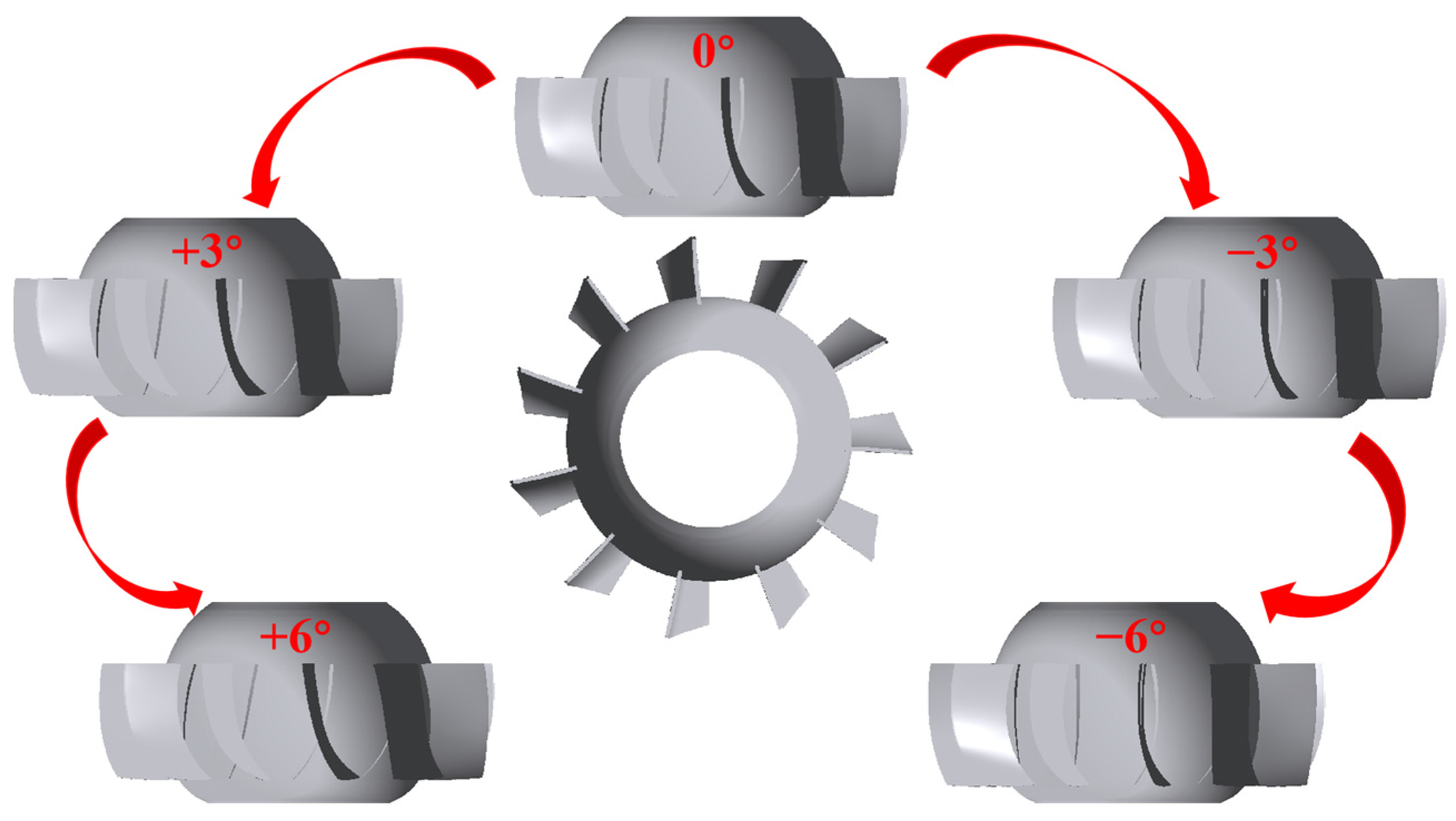
According to the research of a mixed-flow pump in a low-head pumping station, the pump station comprises an elbow-shaped inlet passage, impeller head, servomotor, oil receiver, hydraulic device, guide vane system, outlet passage, and forebay for both the inlet and outlet. The model is composed of the inlet passage, impeller, guide vane assembly, outlet passage, and wheel hub. Specific parameters are shown in

Table 1. Parameters of mixed-flow water pump.

Parameter	Value	Unit
Design Pump Head Hd	7.6	[m]
Design Flow Rate Qd	34	[m3/s]
Shaft Power P	2157.22	[kW]
Rated Rotational Speed nr	125	[r/min]
Total Efficiency η	93.13	[%]
Specific Speed ns	581	[-]
Impeller Blade Number zimp	4	[-]
Vane Blade Number zv	12	[-]

.

The calculation formula for the specific speed is:

$${\mathrm{n}}_{\mathrm{s}}={\displaystyle \frac{3.65n_r\sqrt{Q_d}}{H_d^{0.75}}}$$

(1)

The inlet passage adopts an elbow-shaped inlet pipeline, with a length of 11.2 m and a height of 3 m from the centerline of the first inlet section to the final outlet section (circular outlet section). The transition from the inlet to the outlet is a gradual transition from rectangular to circular.

The mixed-flow impeller has four blades. At the design load, the leading-edge angles of the impeller blades are 40.274°, 72.520°, and 78.168°; the trailing-edge placement angles are 30.875°, 52.462°, and 66.404°; and the impeller diameter is 2950 mm. The original number of fixed guide vanes is 12, the wrap angle is 30°, and the type is a space twisted blade. The leading-edge placement angles are 48.564°, 58.299°, and 65.345° in sections of 0%, 50%, and 100% from the inside out, respectively. The trailing-edge placement angle is 90°. The length of the outlet passage is 27.8 m (from the center of the circular cross-section to the center line of the rectangular cross-section at the end), and the overall passage adopts a gradient type. The specific model used is shown in Figure 1.

2.2. Modified Model

We attempt to transform the fixed guide vane in the guide vane body into an adjustable guide vane, replace the cylindrical hub of the fixed guide vane with a spherical one, and redesign the inlet angle of the adjustable guide vane using a velocity triangle based on the Euler motion equation. We attempted to transform the fixed guide vanes into adjustable guide vanes, replacing the cylindrical hub with a spherical hub and redesigning the inlet angle of the adjustable guide vanes using velocity triangles based on Euler’s equations of motion. As for the predetermined rotation axis, the guide vane can be rotated ±3° and ±6°. According to the right-hand rule, the rotation direction is roughly perpendicular to the paper surface. Clockwise rotation is a negative angle (the leading-edge placement angle of the guide vane increases), and counterclockwise rotation is a positive angle (the leading-edge placement angle of the guide vane decreases), as shown in Figure 2.

2.3. Grid Division

We establish a three-dimensional unsteady flow numerical analysis model for the entire passage, with the fluid domain including an elbow inlet passage, impeller domain, guide vane domain, and siphon outlet passage. Hexahedral and tetrahedral meshes are used to discretize the computational domain. In the orthogonal experiment, five different angles of the impeller were used, with a total of five impeller grids. The guide vane body had a fixed guide vane and five angle-adjustable guide vanes, with a total of six guide vane grids. The grid is shown in Figure 3.

3. CFD Settings

3.1. Computational Fluid Dynamics Equations

In this study, numerical simulations of three-dimensional incompressible fluids are carried out using the Reynolds time-averaged method, under which the continuity, momentum, and total energy equations are given in Equations (2)–(4).

$${\displaystyle \frac{\partial \overline{u_i}}{\partial x_i}}=0$$

(2)

$$\rho {\displaystyle \frac{\partial \overline{u_i}}{\partial t}}+\rho \overline{u_j}{\displaystyle \frac{\partial \overline{u_i}}{\partial x_j}}={\displaystyle \frac{\partial }{\partial x_j}}\left(-\overline{p}{\delta }_{ij}+2\mu \overline{S_{ij}}-\rho \overline{u_i^{\prime }{u}_j^{\prime }}\right)$$

(3)

$${\displaystyle \frac{\partial }{\partial t}}(\rho h_{tot})-{\displaystyle \frac{\partial p}{\partial t}}+{\displaystyle \frac{\partial }{\partial x_j}}(\rho u_j{h}_{tot})={\displaystyle \frac{\partial }{\partial x_j}}\left({\lambda }_t{\displaystyle \frac{\partial T}{\partial x_j}}-\overline{u_j{h}_{sta}}\right)+{\displaystyle \frac{\partial }{\partial x_j}}\left[u_j\left(2\mu \overline{S_{ij}}-\rho \overline{u_i^{\prime }{u}_j^{\prime }}\right)\right]$$

(4)

where $u$ is velocity, $p$ is the pressure, $t$ is time, $\rho$ is density, $T$ is temperature, $x$ is the coordinate component, ${\delta }_{ij}$ is the Kroneker delta, $\mu$ is the dynamic viscosity, $S_{ij}$ is the mean rate of the strain tensor, $h_{sta}$ is static enthalpy, $h_{tot}$ is total enthalpy, and ${\lambda }_t$ is thermal conductivity.

These three equations [23] are the core of numerical simulation methods. They describe the transfer of mass, momentum, and energy in the flow field. By discretizing the equation, important information about the velocity, pressure, temperature distribution, and other aspects of the flow field can be obtained. The model needs to consider the flow characteristics near the wall, taking into account the applicability of different turbulence models to different flow situations and engineering problems. Different degrees of turbulence have different computational complexity and accuracy, and the wall treatment methods are also different. The SST $k-\omega$ model has high accuracy near the wall and saves computational resources. The SST model is based on temperature correction parameters for calculation and can accurately predict the loss coefficient of inviscid flow within five boundary layer thicknesses. It can also accurately predict the uniformity of turbulent flow accumulation areas. This model has a wide range of applications and combines the characteristics of the $k-\epsilon$ and $k-\omega$ turbulence models in free flow, making it suitable for low-Reynolds-number models. Compared to other turbulence models, this turbulence model is more stable and effectively simulates divergent or unstable situations on the wall. In the later stage of this experiment, a large amount of data processing will be carried out, with high computational complexity, limited computing resources, and high computational efficiency. This is suitable for the high computational complexity of this model. Based on the above advantages, this article employs the SST $k-\omega$ turbulence model as the turbulence prediction model. The turbulent flow energy equation $k$ and turbulent dissipation rate equation $\omega$ are expressed as the following equations:

$${\displaystyle \frac{\partial (\rho k)}{\partial t}}+{\displaystyle \frac{\partial \left(\rho u_{i}k\right)}{\partial x_i}}=P_k-{\displaystyle \frac{\rho k^{3/2}}{l_{k-\omega }}}+{\displaystyle \frac{\partial }{\partial x_i}}\left[\left(\mu +{\sigma }_k{\mu }_t\right){\displaystyle \frac{\partial k}{\partial x_i}}\right]$$

(5)

$${\displaystyle \frac{\partial (\rho \omega )}{\partial t}}+{\displaystyle \frac{\partial \left(\rho u_i\omega \right)}{\partial x_i}}=C_{\omega }{P}_{\omega }-\beta \rho {\omega }^2+{\displaystyle \frac{\partial }{\partial x_i}}\left[\left({\mu }_l+{\sigma }_{\omega }{\mu }_t\right){\displaystyle \frac{\partial \omega }{\partial x_i}}\right]+2\left(1-F_1\right){\displaystyle \frac{\rho {\sigma }_{\omega 2}}{\omega }}{\displaystyle \frac{\partial k}{\partial x_i}}{\displaystyle \frac{\partial \omega }{\partial x_i}}$$

(6)

$$l_{k-\omega }=k^{1/2}{\beta }_k\omega$$

(7)

In Formulas (2) to (7), $\rho$ is the fluid density; $k$ is the turbulence kinetic energy per unit mass; $\omega$ is the specific kinetic energy dissipation rate; $t$ is time; $x$ is the coordinate; $p$ is pressure; $\mu$ is the dynamic viscosity coefficient; $u_i$ (I = 1, 2, 3) is the velocity component of the fluid; $f_i$ is the mass force component; ${\mu }_t$ is the eddy viscosity coefficient; $l_{k-\omega }$ is the turbulence scale; $F_1$ is a blending function; and $C_{\omega }$, ${\sigma }_k$, ${\sigma }_{\omega }$, ${\sigma }_{\omega 1}$, ${\sigma }_{\omega 2}$, $\beta$ are the constants.

3.2. CFD Parameter Adjustment

Numerical simulation calculations rely on ANSYS CFX 2023 R1commercial software and relevant theories of computational fluid dynamics. We specify the simulation problem, including determining the geometric shape, flow type, boundary conditions, and fluid medium. In order to better explore the effects of the flow rate, impeller angle, and guide vane angle on the hydraulic efficiency of mixed-flow pumps, we conducted orthogonal experiments. Based on the consideration of the above issues, the turbulent energy of mixed-flow water pump with 2°, 0°, −2°, −4°, and −6° impeller blades and ±6°, ±3°, and 0° adjustable guide vanes under typical operating conditions was studied and calculated. This step numerically simulated water in a fluid medium of 25 °C at a reference pressure of 1 atm. We established the inlet surface of the elbow inlet passage as the inlet of the fluid domain and set the mass flow rate as the inlet boundary condition. Regarding others, we determined the outlet surface of the outlet channel as the outlet of the fluid domain and set it as an outlet boundary condition with average static pressure. The outlet is connected to the atmosphere, with a pressure value of 0 Pa. The impeller is the only rotating component with a rotation speed of 125 r/min. The dynamic and static reference frame is set between the impeller and the inlet passage, as well as between the impeller and the guide vane, while the frozen rotor reference frame is set between the other components. A universal grid-connected GGI model is used for data transmission between different interfaces. We choose SST $k-\omega$ for the turbulence model. The boundary conditions between the walls are all smooth and slip-free. Regarding the calculation problem of the model, a steady simulation calculation is adopted, with minimum iteration steps of 1000 in the steady calculation. The convergence criterion of the numerical simulation is the continuity equation, and the root mean square residuals of the momentum equation and energy equation are less than 1 × 10⁻⁵.

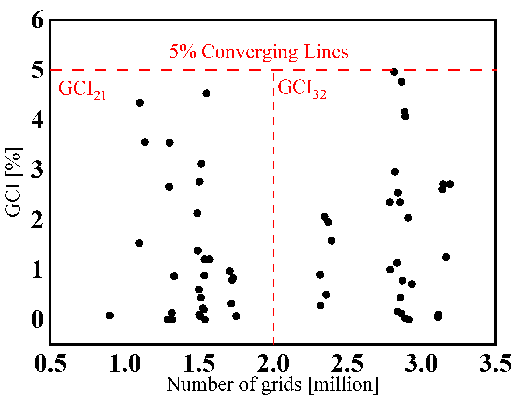
3.3. Grid Independence Test

The grid independence test is a crucial step in CFD numerical simulation, as it plays a crucial role in the accuracy and reliability of the simulation. In this article, orthogonal experiments are used to screen the primary and secondary factors. A three-factor, five-level orthogonal table is used in the orthogonal experiment. Two control experiments are conducted, with a total of 30 matching models for impeller and different types or angle guide vane. Among of them are 5 models for fixed guide vanes and 25 models for adjustable guide vanes. Due to the subsequent research focus on the performance of the impeller and guide vane, a full passage simulation was adopted. The number of grids in the elbow inlet passage and the siphon outlet passage remained unchanged, with 179,148 and 281,164, respectively. Grid independence was verified for 30 models, and the fluid domains of the impeller and guide vane were discretized, refined, and sparse, resulting in a total of 90 sets of grids. There were three sets of grids with significant resolution in the models used in each orthogonal experiment. The GCI [24] value is shown in Figure 4.

After analysis, it can be seen that the values converged at a moderate level as the number of grids increased. However, due to the later calculation of models with multiple operating conditions and multiple combinations of dynamic and static blades, in order to, as much as possible, save certain computational resources without sacrificing computational accuracy, it was ultimately decided to use each moderate-level grid as the choice for their respective schemes.

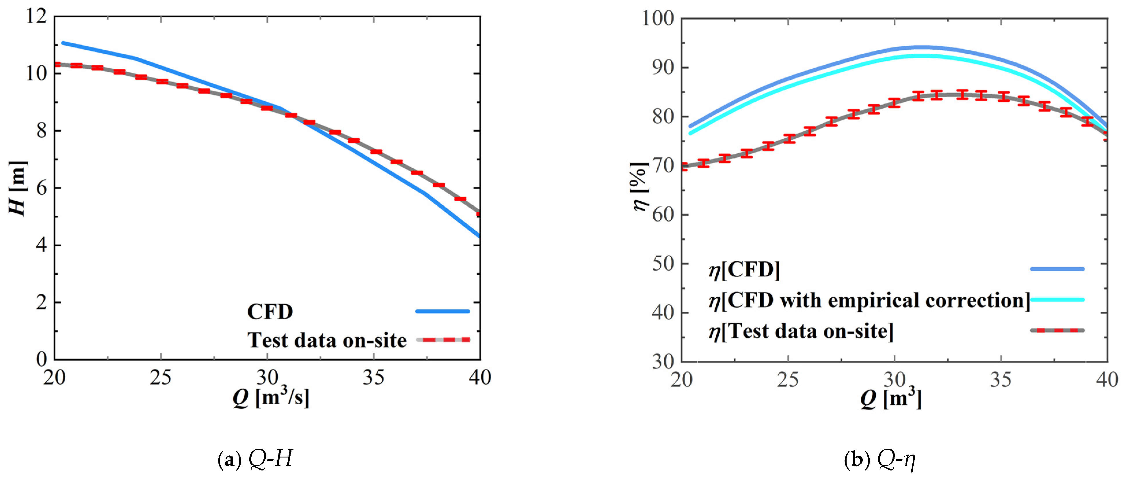
4. Performance and Verification

In this study, by controlling the flow inlet boundary conditions at the inlet face of the model inlet passage, the working conditions from the 0.6 Q_d~1.2 Q_d rated flow rate were calculated. By studying the external characteristic curves, we can verify that mathematical and physical models had similar characteristics to real machines. Through CFD post-processing, we read the pressure value of the interface to find the hydraulic loss of each component, then finally read the head and efficiency values. The external characteristic curve is shown in Figure 5.

In Figure 5, η [CFD] is the numerical value read from CFD post, with the specific formula as follows [25]:

$$\eta [CFD]=(p_{van-ef}-p_{impeller-if})Q/M\omega$$

(8)

where $p_{van-ef}$ is the vane export flange total pressure, $p_{impeller-if}$ is the impeller inlet flange total pressure, M is the impeller shaft torque, and $\omega$ is the angular velocity.

Since the efficiency calculated by CFD does not take into account mechanical and volumetric losses, it is corrected by an empirical equation, which is given as:

Mechanical efficiency:

$${\eta }_{\mathrm{m}}=1-0.07{\displaystyle \frac{1}{{\left(n_s/100\right)}^{7/6}}}$$

(9)

Volumetric efficiency:

$${\eta }_{\mathrm{v}}={\displaystyle \frac{1}{1+{0.68n_s}^{-2/3}}}$$

(10)

Total efficiency:

$${\eta }_h=\eta [CFD]$$

(11)

$$\eta ={\eta }_h{\eta }_m{\eta }_v=\eta [CFD with empirical correetion]$$

(12)

${\eta }_h$ is the CFD-calculated hydraulic efficiency of 93.13%, ${\eta }_m$ is the mechanical efficiency of 99.10%, ${\eta }_v$ is the volumetric efficiency of 99.03%, and the total efficiency correction value is 98.14% for the figure of CFD with empirical correction. It can be seen that the head and efficiency curves are in line with the basic law, and the calculated value and the real value of the data are basically fitted to the model to achieve the hydraulic performance.

5. Orthogonal Experiments

5.1. Experimental Design

The dimensions and mesh division of each component model are described above. During the actual operation of the pumping station, operating condition changes are manifested as the flow rate changes. The flow rate affects the head and efficiency of the pump. Either too small or too large a flow rate can cause a decrease in efficiency. The positive angle rotation of the adjustable impeller can improve the boosting efficiency, and the head will be significantly increased. But at the same time, the torque of the impeller increases, which will cause an increase in power while maintaining the rated speed of the original motor. And the overall efficiency will decrease. The use of an improved rotating adjustable guide vane instead of a traditional fixed guide vane can be adjusted according to changes in the impeller angle.

In order to explore the coupling effects of the flow rate, impeller angle, and guide vane angle on the hydraulic efficiency of high-specific-speed mixed-flow pumps, two schemes were designed in this orthogonal experiment. The first type is a fixed guide vane, and the second type is an adjustable guide vane with an improved design. This experiment uses five flow rates (working conditions) from small to large, namely 0.6 Q_d (20.4 m³/s), 0.8 Q_d (27.2 m³/s), 1.0 Q_d (34.0 m³/s), 1.2 Q_d (40.8 m³/s), and 1.4 Q_d (47.6 m³/s). The first fixed guide vane scheme adopts a guide vane angle of all 0°, while the second adjustable guide vane scheme adopts five guide vane angles: +6°, +3°, 0°, −3°, and −6°, respectively. The five impeller angles are +2°, 0°, −2°, −4°, and −6°, respectively. Taking the flow rate, guide vane angle, and impeller angle as experimental influencing factors, five levels are set for each factor without considering the interaction between factors. The specific orthogonal experimental plan is shown in

Table 2. Three-factor, five-level orthogonal table for adjustable guide vane.

Orthogonal Design	A Flow Rate (m3/s)	B Guide Vane Angle (°)	C Impeller Angle (°)
1	20.4	+6	+2
2	20.4	+3	0
3	20.4	0	−2
4	20.4	−3	−4
5	20.4	−6	−6
6	27.2	+6	0
7	27.2	+3	−2
8	27.2	0	−4
9	27.2	−3	−6
10	27.2	−6	+2
11	34	+6	−2
12	34	+3	−4
13	34	0	−6
14	34	−3	+2
15	34	−6	0
16	40.8	+6	−4
17	40.8	+3	−6
18	40.8	0	+2
19	40.8	−3	0
20	40.8	−6	−2
21	47.6	+6	−6
22	47.6	+3	+2
23	47.6	0	0
24	47.6	−3	−2
25	47.6	−6	−4

Set all factor B values to 0° for a fixed guide vane.

.

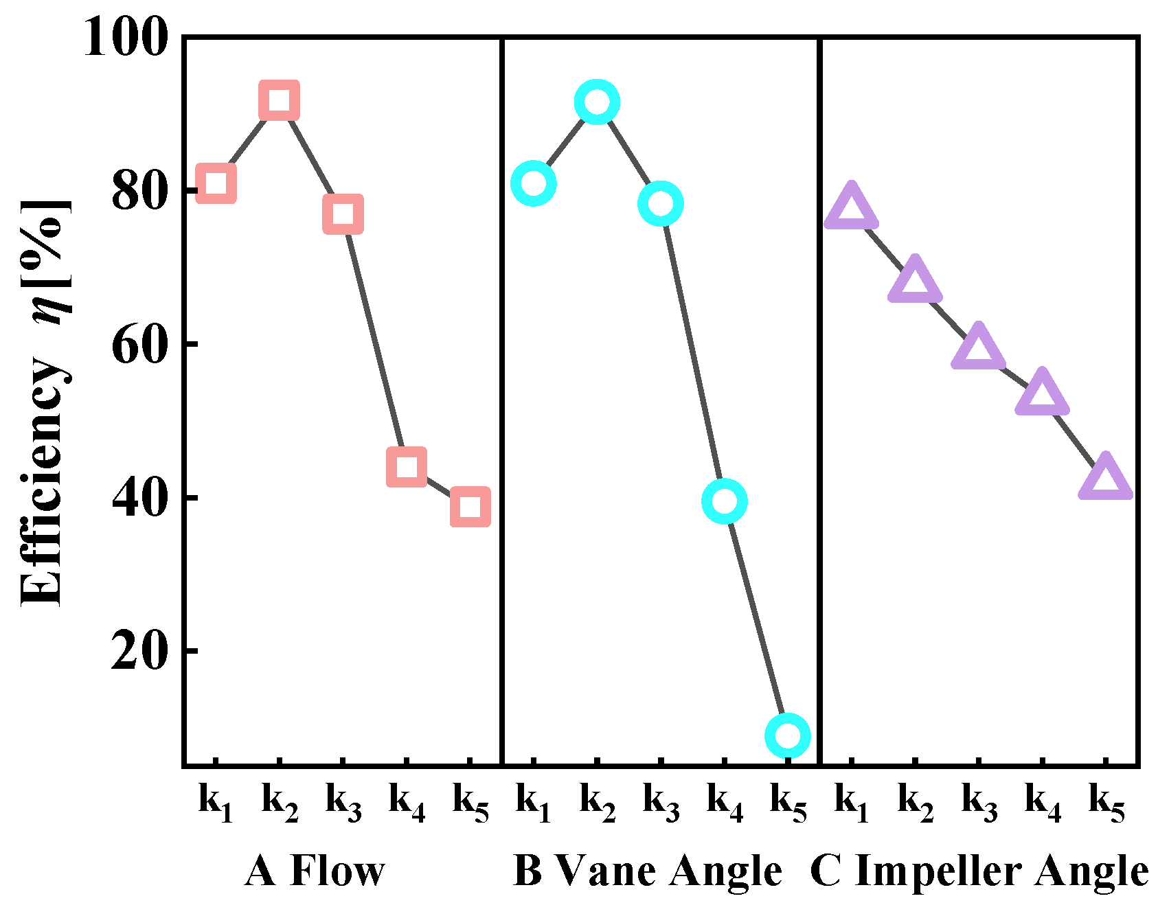
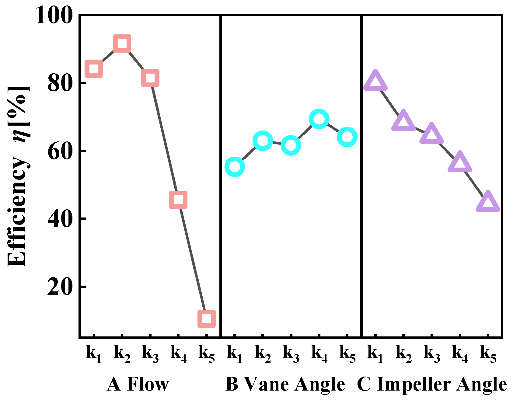
5.2. Analysis of Orthogonal Experimental Results

The experimental results can achieve the following goals through range analysis: 1. evaluate the reliability of experimental data and determine the primary and secondary factors that affect the experimental results to improve experimental efficiency; 2. determine the relationship between experimental factors and experimental results, and be able to predict and optimize the experimental results; 3. the influence of experimental factors on experimental results provides ideas for controlling experiments.

5.2.1. Analysis of Fixed Guide Vane Scheme

According to Figure 6 of the range analysis of the fixed guide vane orthogonal experiment, it can be concluded that the primary and secondary relationships of the factors are B > A > C. From the results of range analysis alone, we can see that the angle of the guide vane has a significant impact on efficiency. However, since the angle of the guide vane in this experiment is fixed at 0°, the highest R_B value does not necessarily indicate that changes in the guide vane angle will have a significant impact on efficiency. But the highest R_B can indicate that the adaptability of the fixed guide vane angle to the increase in factor A (flow rate) and the rotation of factor C (impeller angle) is extremely poor, which is why the maximum range occurs.

Due to the angle of the fixed guide vane remains constant at 0°, the influence of factor B (guide vane angle) on the efficiency can be eliminated.

The change in efficiency caused by factor B (guide vane angle) fluctuates due to changes in the levels of other factors. According to Figure 7, it can be clearly seen that as the angle of the impeller increases with factor C (impeller angle), the efficiency of the pump steadily decreases with changes in angles of +2°, 0°, −2°, −4°, and −6°. The increase in factor A (flow rate) will first increase and then decrease the efficiency, which is consistent with our current research on high-specific-speed mixed-flow pumps. With respect to factor C (impeller angle), as the impeller angle rotates from positive to negative, it can be seen that the k-avg value continuously decreases. This indicates that its adaptability to the flow rate has deteriorated, leading to a decrease in pump efficiency. Figure 7 shows the influence of factor A’s flow rate on the five impeller angle levels for factor C (impeller angle).

On the left side of the small-flow area (rated flow rate A₃ 34 m³/s), the operating efficiency of the negative-angle impeller is higher, especially at A₁ 20.4 m³/s, where the efficiency appears as C₅ > C₄ > C₃ > C₂ > C₁. On the right side of the high-flow area (rated flow A₃ 34 m³/s), the operating efficiency of the positive-angle impeller is higher. At A₄ 40.8 m³/s, the efficiency shows a phenomenon of C₁ > C₂ > C₃ > C₄ > C₅. The efficiency attenuation of the negative-angle impeller is particularly severe in high-flow areas. Taking factor C₅ as an example, at A₁ (20.4 m³/s), the efficiency was 89.06%, but at the rated flow rate A₃ (34.0 m³/s), it increased to 29.87%, almost reducing by 2/3. The remaining negative angles of C₃ and C₄ also experienced a sharp drop. This means thatthe negative-angle impeller can maintain high efficiency in small-flow areas, but exceeding the rated flow rate and further increasing the flow rate will cause a sharp decrease in efficiency. The positive-angle impellers still maintain a certain efficiency in high-flow areas, but their efficiency is relatively low in small-flow areas compared to negative-angle impellers. The 0° impeller combines two characteristics. But it cannot be ignored that the pattern is generated at a 0° guide vane. The efficiency of a mixed-flow pump with a fixed guide vane is more sensitive to changes in operating conditions.

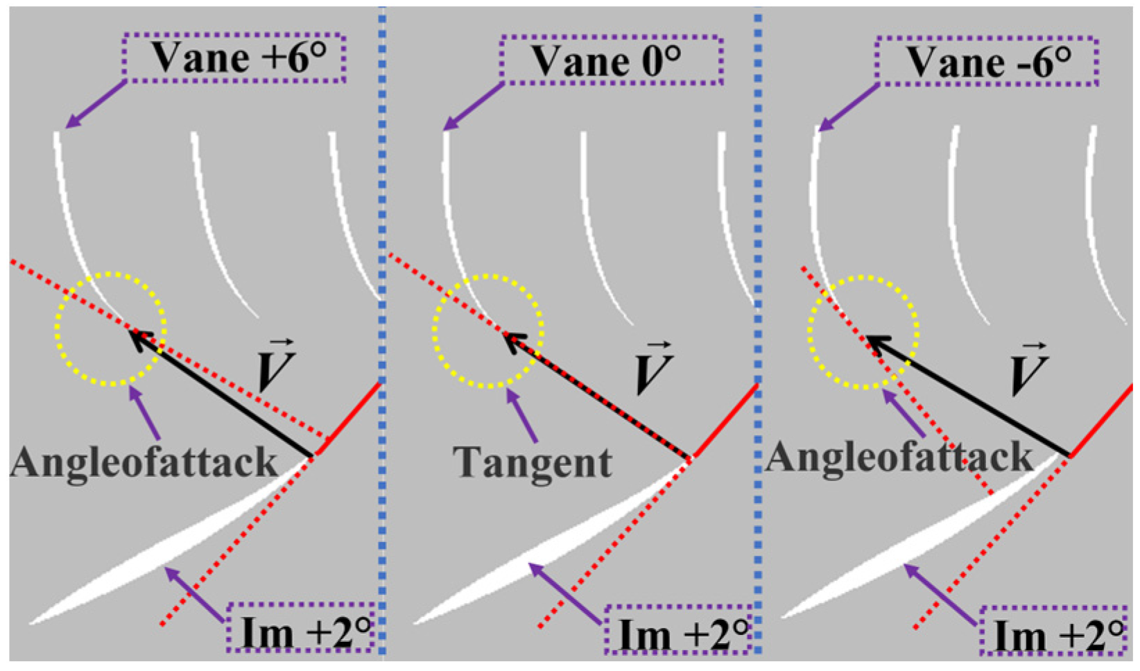
5.2.2. Analysis of Adjustable Guide Vane Scheme

After analyzing the fixed guide vane, we found that the angle of the fixed guide vane was not suitable for an operation with variable working conditions and an adjustable impeller. After improving the design of the guide vane, the angle of the guide vane could be adjusted, as shown in Figure 2. The results of the orthogonal experiment are shown in Figure 8.

According to the range analysis figure, it can be concluded that the primary and secondary relationships of the factors were A > C > B. After using the adjustable guide vane, the impact of the factor (A flow rate) on the efficiency showed an absolute advantage among the three factors. This is because, in orthogonal experiments, there is a certain degree of randomness in the angle matching of the guide vane and the impeller. The angle match between the guide vane and the impeller greatly affects the flow of water through the system. Once mismatched, it can cause serious phenomena, such as separation vortices, impeller outflow impact on guide vane inlet, and blade passage blockage, that affect pump efficiency. In the orthogonal experiment with a fixed guide vane angle in Section 5.2.1, the range of factor C (impeller angle) is R_c35.31. In this orthogonal experiment with an adjustable-angle guide vane, the range of factor C (impeller angle) is R_c35.66, which is basically consistent. In the analysis of Section 5.2.1, we believe that the fixed guide vane 0° has a range value R_B of 82.64, indicating that the fixed guide vane 0° cannot adapt well to changes in the impeller angle and flow rate caused by changes in the operating conditions. Therefore, there are significant differences in efficiency and range. The guide vane was improved to be adjustable, which could match to some extent with the impeller after angle adjustment. Although it was not a perfect match, the random matching of the dynamic and static blade angles reflected a relatively uniform distribution in the k-avg value. There was no significant range observed in the first experiment. In the past, the idea of orthogonal experiments often relied on large fluctuations in the value of k to determine which factor and level were most suitable. But it is difficult for us to analyze which angle is the so-called optimal angle because the flow rate, guide vane angle, and impeller angle have a coupled relationship. Perhaps only one combination of moving and stationary blades can achieve the highest efficiency under each operating condition (flow rate). After using the adjustable guide vane, the k-avg value did not change significantly with changes in flow rate and impeller angle, indicating that the adjustable guide vane improved the adaptability of the mixed-flow pump to changes in operating conditions.

According to Figure 8, the k-avg value of factor A showed a consistent trend compared to Figure 6, the difference being that the efficiency was very low at k₅, only 10.60%, and k₅, as shown in Figure 6, was 38.76%. This phenomenon can be analyzed based on the three-level shape of the velocity. As shown in Figure 9, with the increase in flow rate, the absolute flow rate inside the pump increased. Due to the constant rotational speed, the circumferential velocity of liquid particles at various locations on the impeller did not change, resulting in a change in the direction of the absolute flow velocity. The specific variation pattern can be obtained from the orthogonal table and velocity triangle analysis: as the flow rate increased and the impeller rotated at a positive angle, the absolute speed direction rotated clockwise, as shown in Figure 9; when the flow rate decreased and the impeller rotated at a negative angle, the absolute speed direction rotated counterclockwise, as shown in Figure 9. According to Figure 2, showing the rotation direction of the guide vane, when the flow rate increases, the guide vane needs to rotate in the negative direction (clockwise rotation on the vertical paper surface), and when the flow rate decreases, the guide vane needs to rotate in the positive direction (counterclockwise rotation on the vertical paper surface). When adjusting the positive angle of the impeller, the negative angle of the guide vane can be matched, and when adjusting the negative angle of the impeller, the positive angle of the guide vane can be matched. This is the physical problem with mismatched dynamic and static blades in adjustable-blade mixed-flow pumps. And as shown in Figure 9, we used an adjustable-angle guide vane. With the angle of the impeller or the flow rate increasing, when their angles do not match, the absolute velocity direction forms an angle of attack with the tangent extension line of the guide vane’s leading edge. When the impeller angle is regular (+2° in the figure) and the flow rate is fixed (axial flow velocity is fixed), theoretically, by rotating the guide vane towards a negative angle, the tangent line of the leading edge of the guide vane can correspond to the direction of the pressurized water flow flowing out of the impeller. This can not only reduce the hydraulic loss of water flow in the guide vane body, but also reduce the problem of water flow blockage in the boundary area due to the smooth flow of the impeller, which is necessary for large-sized, high-specific-speed pumps. At the same time, there are also two situations shown in Figure 9, which are the positive and negative angles of attack caused by the mismatch of the tangent lines of the guide vane inlet profile. After simple mathematical calculations, the k₅ of factor A (flow rate) forms different degrees of positive angles of attack with five different guide vane angles. Under the conditions of k₁ and k₂ of factor A (flow rate), there is also a negative impact angle after a simple calculation, but its efficiency does not sharply decrease. The research on and discussion of this issue will be presented later. From the perspective of factor B (guide vane angle), it can be seen from Figure 8 that its efficiency was almost maintained at a certain level. Even though its range R_B was only 14.07 compared to 82.64 of the range R_B in the orthogonal experiment described in Section 5.2.1, we still believe that the angle of the guide vane can greatly affect the efficiency of the pump.

In the orthogonal experiment, we used a three-factor, five-level orthogonal table and found that the mismatch between the moving and stationary blades caused the efficiency of the water pump to drop sharply to zero, making it unable to operate under high-flow conditions; the impact of changes in the impeller angle on the pump efficiency was not only stable but also limited; and the change in the guide vane angle had a certain effect on the improvement of the efficiency.

6. Matching Analysis of Moving and Stationary Blades

In order to verify the effects of the flow rate, guide vane angle, and impeller angle on the efficiency of the pump, we used some matching models of moving and stationary blades with adjustable guide vanes in an orthogonal table for an orthogonal experiment. In order to further investigate the effect of variable-angle adjustable guide vanes on improving the efficiency of mixed-flow pumps, we used a combination of improved design with adjustable guide vane angles of ± 6°, ± 3°, and 0° and impeller angles of +2°, 0°, and −2°. The flow rates were set to 0.6 Q_d, 0.7 Q_d, 0.8 Q_d, 0.9 Q_d, 1.0 Q_d, 1.1 Q_d, and 1.2 Q_d. The first boundary condition of Dirichlet is as follows:

Inlet of inlet passage:

$$\mathit{Q}=\mathit{Q}\mathit{V},\mathit{V}={\mathit{V}}_{\mathit{c}},{\displaystyle \frac{\partial \mathit{p}}{\partial \mathit{x}}}=0$$

(13)

Outlet of water outlet passage:

$$\mathit{p}={\mathit{p}}_{\mathit{c}},{\displaystyle \frac{\partial \mathit{v}}{\partial {\mathit{x}}_{\mathit{i}}}}=0$$

(14)

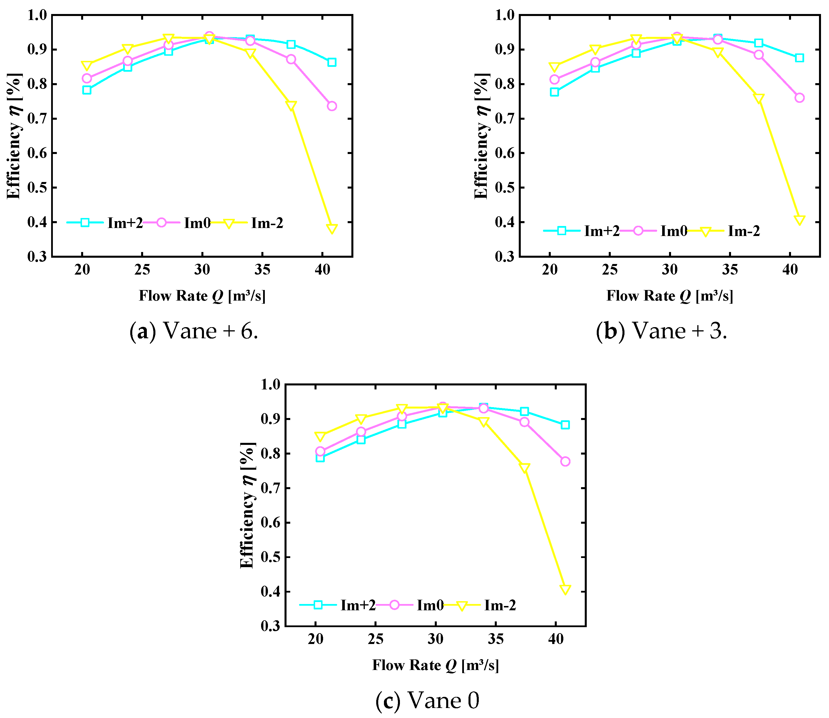
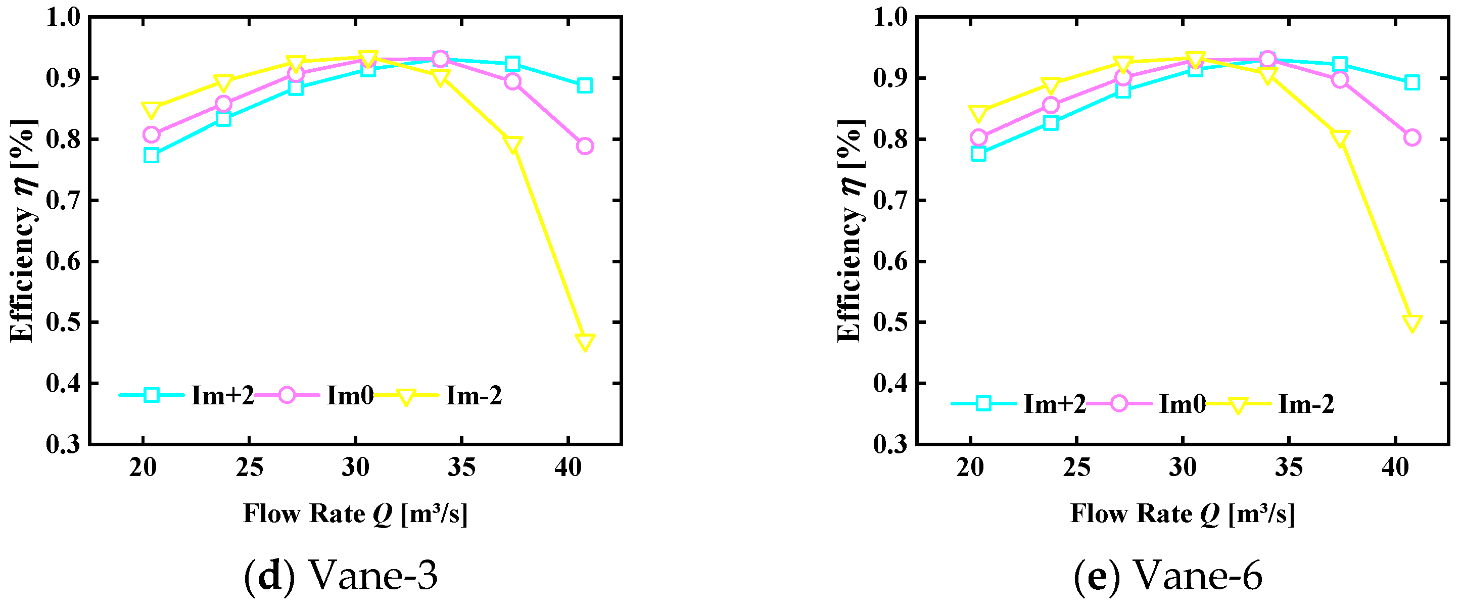
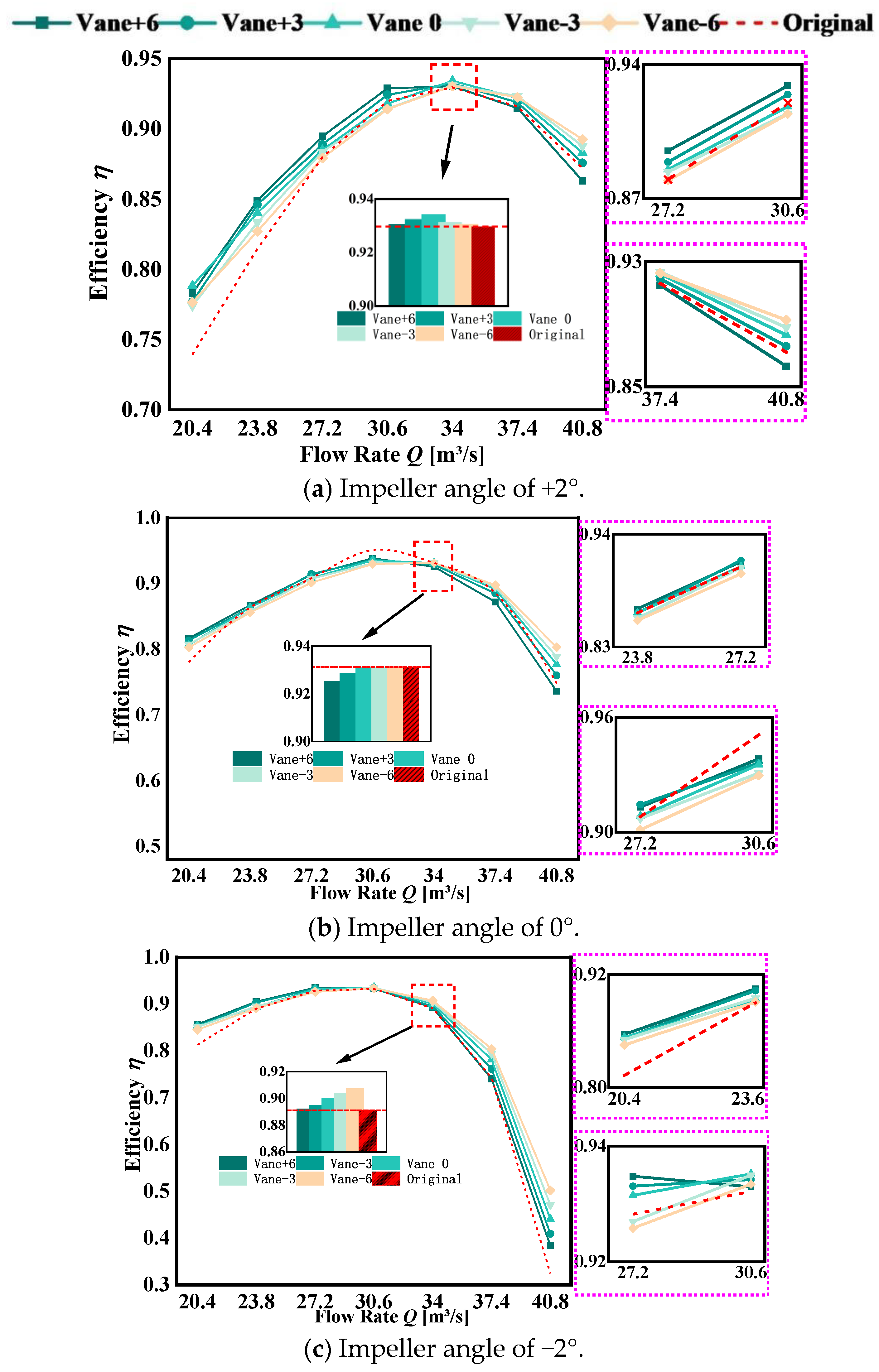
6.1. Analysis of Single Flow Efficiency Curve

We controlled changes in operating conditions through the volumetric flow rate, as analyzed in the previous orthogonal experiment. Our GCI validated the model’s stability for five different guide vane angles and five different impeller angles. In the orthogonal experiment, we found that the matching effect with the existing five adjustable guide vane angles was not good when the impeller angles were −4° and −6°. Therefore, models with impeller angles of −4° and −6° were excluded, and only models with impeller angles of +2°, 0°, and −2° and adjustable guide vane angles of ±6°, ±3°, and 0° were studied here. The fifteen models used in this study have already been included in the previous GCI grid validation. There is no need to verify them again this time. After post-processing, reading, and organizing the calculation results, the flow efficiency curve was obtained, and is shown in Figure 10.

From Figure 10, it can be seen that different impeller angles at the same guide vane angle resulted in different positions of the highest efficiency point. The change in efficiency was related to the rotation angle of the impeller: according to the size of traffic, the order in which the highest efficiency point appeared was impeller −2°, impeller 0°, and impeller +2°. The highest efficiency occurred when the impeller operated at a negative angle in a small-flow area. The highest efficiency was achieved when the impeller operated at a positive angle in high-flow areas. At the rated operating point, the zero-degree impeller had the highest efficiency.

During the actual operation of the pumping station, the opening adjustment of the guide vane was intended to match the opening adjustment of the impeller. Therefore, the efficiency curves under the same impeller angle but different guide vane openings were organized as shown in Figure 11.

Figure 11a shows the flow efficiency when the impeller angle was +2° and matched with five different guide vane angles. At low-flow operating points of 20.4 m³/s, 23.8 m³/s, 27.2 m³/s, and 30.6 m³/s, the guide vane with the best matching angle with the impeller was +6°, because its highest efficiency operating condition occurred three times. The worst match was the −6° guide vane, as its efficiency was always the lowest. The average efficiency of the +6° guide vane at these four operating points was about 1.47% higher than that of the −6° guide vane. And the average efficiency of the +6° guide vane at these four operating points was about 2.55% higher than that of the original guide vane model. The combination with the highest efficiency at 0.6 Q_d matched the 0° guide vane. The efficiency of the original guide vane model gradually exceeded that of the modified model through an increase in the flow rate from 0.8 Q_d to 0.9 Q_d. The efficiency of the original model exceeded the −6°, −3°, and 0° guide vanes in sequence. At the rated operating point, the most efficient one was no longer the +6° guide vane, but the 0° guide vane, which was 3.80% more efficient than the former at this operating point. However, from Figure 11a, we can see that the efficiency of the original model was the lowest at the rated operating point, and the modified guide vane 0° model was 0.40% higher than the original model. As the flow rate increased to the high-flow operating point (37.4 m³/s, 40.8 m³/s), the highest efficiencies were −3° and −6°. But at this point, the model with the lowest efficiency was the +6° model, which had a difference of 0.86% in efficiency compared to −3° and a difference of 2.96% compared to −6°. With model conversion from low-traffic to high-traffic areas and from minimum efficiency to maximum efficiency, the highest-efficiency model in small-flow areas became the lowest-efficiency model when entering large-flow areas, while the lowest-efficiency model in the low-flow area became the highest-efficiency model in the high-flow area.

Figure 11b shows the flow efficiency when the impeller angle was 0° and matched with five different guide vane angles. The best match between the impeller angle at low-flow operating points of 20.4 m³/s, 23.8 m³/s, 27.2 m³/s, and 30.6 m³/s was the guide vane model of 6°. It had the highest efficiency at three operating points (at 27.2 m³/s, the efficiency was only 0.13% lower than +3°) and the lowest efficiency is the −6° guide vane model. The average efficiency of the 6° guide vane at these three operating points was about 1.15% higher than that of the −6° guide vane. However, as the flow rate increased from 0.8 Q_d to 0.9 Q_d, the efficiency of the original model sequentially exceeded the 0°, 3°, and 6° guide vanes. At the rated operating point, it was evident that the highest efficiency was achieved by the original model at 93.13%, while the lowest efficiency was achieved by the +6° guide vane, with a difference of 0.6% between the two. As the flow rate increased to 37.4 and 40.8, the efficiency of the −6° guide vane became the highest, and the efficiency of the +6° guide vane became the lowest, with an average difference of 4.62% between them.

Figure 11c shows the flow efficiency diagram after matching with five different guide vane angles at an impeller angle of −2°. The best match for the −2° impeller in the low-flow area was still the +6° guide vane, and the worst match was still the −6° guide vane. At the rated operating point, the model with the highest efficiency was the −6° guide vane. In the high-flow region, the efficiency decreased rapidly with the increasing flow rate, the highest efficiency changed to −6°, and the lowest efficiency changed to +6°.

Through the above analysis, we noticed that the adjustment of the impeller angle affected the distribution of the pump efficiency zone. When the impeller rotated at a positive angle, the high-efficiency area of the pump moved to the right, making it more adaptable to high flow rates. The pump was still able to maintain a high-efficiency operation in the high-flow-rate area. But as the flow rate decreased, the efficiency of the water pump decreased by about 15%. When the impeller rotated at a negative angle, the high-efficiency zone moved to the left. At this time, the pump maintained high efficiency when working in the small-flow zone, which was more suitable for operating in the small-flow aera. And with the flow rate increasing, the efficiency of the water pump dropped sharply by about 50%. The adjustment of the guide vane angle also had an impact on the efficiency of pumps operating at the same impeller angle: the efficiency of the 6° guide vane model was relatively high in small-flow areas, and as the flow rate increased, the efficiency of the −6° guide vane model was higher in large-flow areas. The sensitivity of efficiency to mismatched guide vane angles varied with different impeller angles. When the impeller was adjusted to a positive angle, it was more sensitive to the mismatch between the moving and stationary blades in the small-flow area. The efficiency difference was greater when the guide vanes were at different angles, and the mismatch between the moving and stationary blades had a more significant impact in the high-flow area when the impeller was adjusted towards a negative angle.

Based on the velocity triangle theory, we can determine that, during the transition process from small-flow area to large-flow area, the theoretical highest-efficiency curves at each operating point should be 6°, 3°, 0°, −3°, and −6° in sequence. However, we noticed more significant changes in the curves of 6° and −6° in the graph. The selection interval of our operating points was every 0.1 Q_d (3.4 m³/s), so the large interval resulted in poor conversion of 3°, 0°, and −3°. However, we noticed a trend of changes in the sub-graphs of Figure 11a–c.

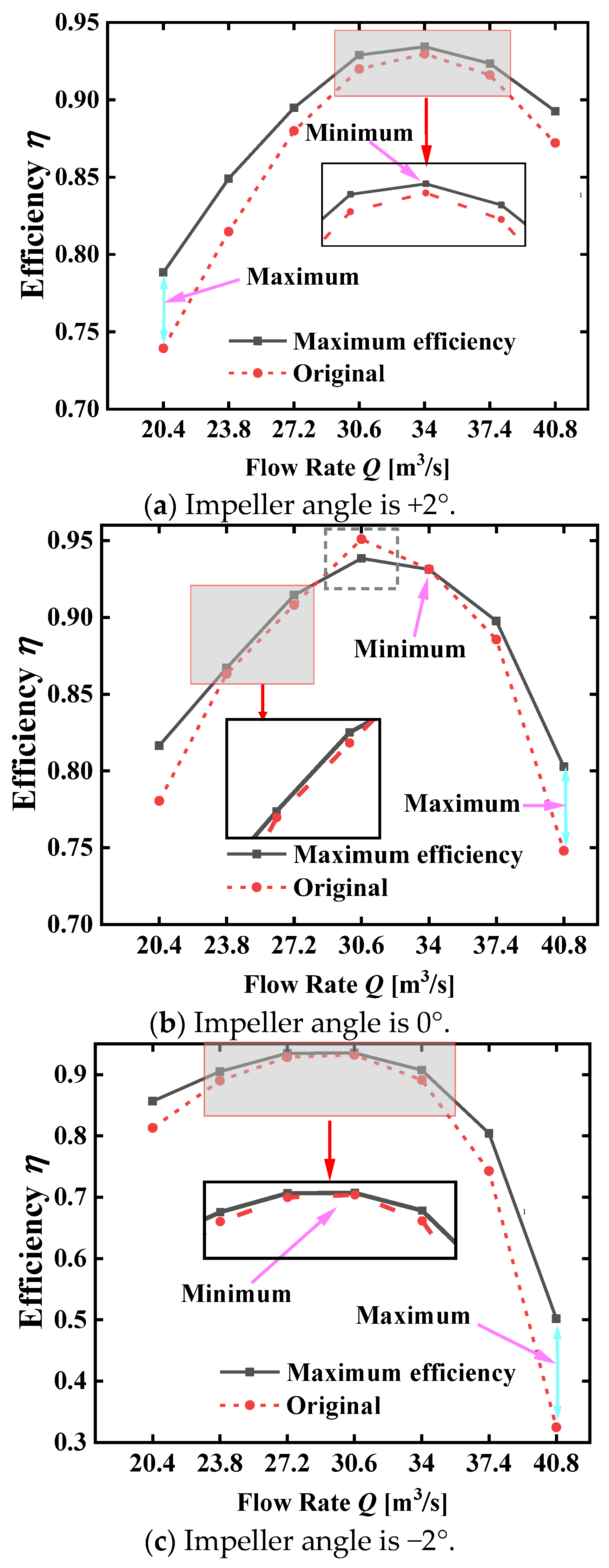
6.2. Analysis of Comprehensive Efficiency Curve

After the analysis in 6.1, we discovered the pattern of matching between the moving and stationary blades. However, in the actual operation process of a pump station, the impeller angle often rotates to a certain angle according to the water regulation task (the operating area changes) and works at this angle for a considerable period of time. During the flood season, the head decreases but inflow increases, so the flow rate of the pump station increases. The impeller needs to be adjusted at a positive angle to shift the efficiency curve to the right as a whole so that the efficiency area remains at the high-flow operating point. During the dry season, the head increases but inflow decreases, and the flow rate of the pump station decreases. The impeller needs to be adjusted towards a negative angle to shift the efficiency curve to the left as a whole, keeping the high-efficiency zone at the low-flow operating point.

According to the operating rules of the pumping station, we organized and combined the maximum efficiency points of different guide vane openings at the same impeller angle to form a comprehensive efficiency diagram of the adjustable guide vane at a certain impeller angle, as shown in Figure 12.

According to Figure 12, the different high-efficiency zones can be clearly seen. When the impeller angle was 2°, the high-efficiency zone was between 30.6 m³/s and 40.8 m³/s, and it was still able to maintain an efficiency close to 90% at 40.8 m³/s. When the impeller angle is 0°, the efficiency range was between 27.2 m³/s and 37.4 m³/s, but when the flow rate exceeded 37.4 m³/s, there was a significant decrease in−34 m³/s, and there was a significant decrease in efficiency when the flow rate exceeded 34 m³/s. Comparing and analyzing the efficiency curve of the red original fixed guide vane (0 opening), the trend of the efficiency curve was almost the same as that of the adjustable guide vane. This indicates that the angle of the impeller had a significant impact on the efficiency curve of the water pump, which can also be seen from the range analysis of the impeller factor in the orthogonal experiment. Figure 13 was formed by cutting and organizing the highest-efficiency curve based on the impeller angles of +2°, 0°, and −2°. It can be seen that the change in the opening of the guide vane also significantly improved the efficiency. When the impeller angles were 2°, 0°, and −2°, the comprehensive efficiency reached up to 4.90%, 5.48%, and 17.71% higher than when using a fixed guide vane. The comprehensive efficiency values were, on average, 2.00%, 1.43%, and 4.61% higher than when using a fixed guide vane.

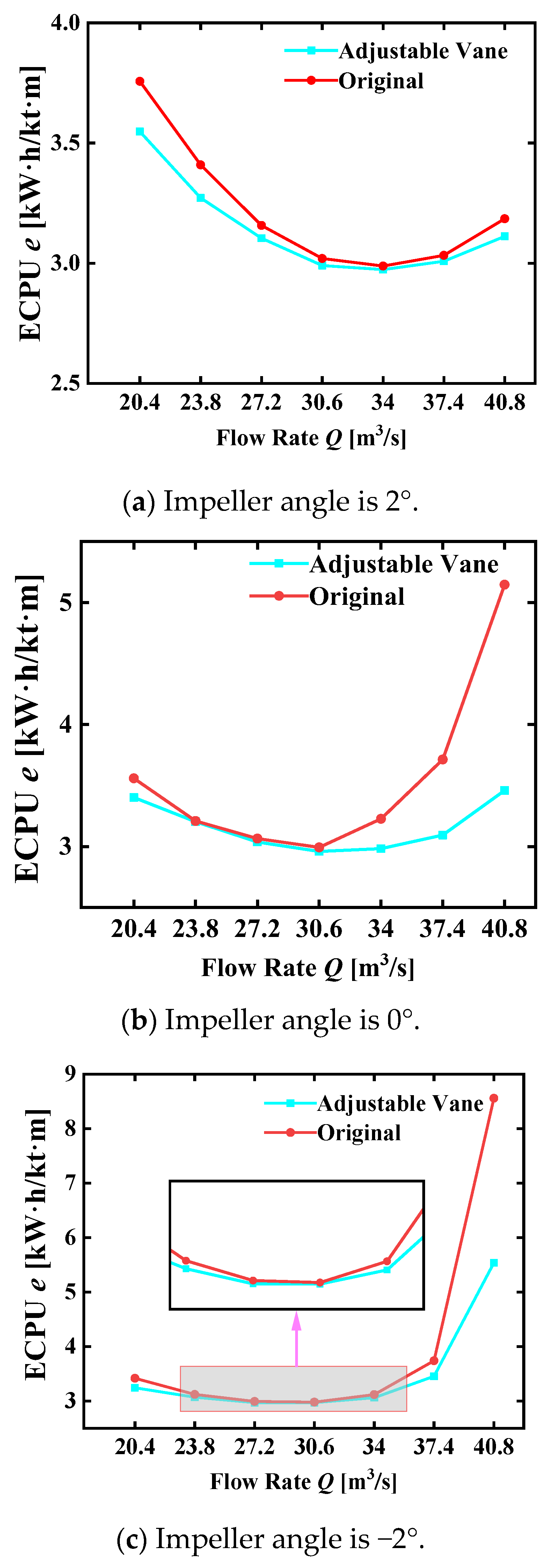
6.3. Energy Consumption Analysis

High-specific-speed guide vane mixed-flow pumps are mainly used in low-head water-regulating pump stations with the following two characteristics: 1. long running time, almost non-stop throughout the year; and 2. the unit has a large size and high power consumption during operation. These two characteristics have a significant impact on energy consumption for pumping stations using high-specific-speed guide vane mixed-flow pumps. Next, by leveraging the energy consumption indicator—energy consumption per thousand tons per meter—in pump station management, we analyze the energy consumption performance of this unit with an adjustable guide vane in comparison to the original unit. The energy consumption formula is as follows:

$$\mathit{e}=\mathit{P}/3.6\mathit{Q}\mathit{H}{\eta }_{\mathit{m}}$$

(15)

• $\mathit{e}$—Energy consumption, kW·h/(kt·m);
• $\mathit{Q}$—Flow rate of water pump under different working conditions, m³/s;
• $\mathit{P}$—Power of water pump under different working conditions, kW;
• $\mathit{H}$—Head of water pump under different working conditions, m;
• ${\mathit{\eta }}_{\mathrm{m}}$—Motor efficiency, [%].

In order to pursue more realistic energy consumption data, we read the power value in CFD as the shaft power and corrected it for motor efficiency. The unit used a 10 kW vertical synchronous motor with high efficiency. After being corrected by 98%, the corresponding energy consumption values were calculated, and they are summarized in the following figure:

According to the energy consumption chart in Figure 14, we can see that the pump with the adjustable guide vane had significantly improved energy consumption compared to the original model in both low-flow and high-flow operating conditions. From Figure 14a, after the transformation, the overall energy consumption significantly decreased, and the operating point with an average reduction effect was the rated operating point (Figure 14b). Except for the 0.9 Q_d operating point, the energy consumption at other operating points decreased, with a particularly significant reduction effect of 1.2 Q_d. From Figure 14c, it can be seen that the effect of reducing energy consumption was not significant, but the energy consumption reduction effect was significant under high-flow conditions. We noticed that under extreme operating conditions, the energy consumption curve of the original model showed a sharp increase when the impeller angle was 0° or −2°. However, after being transformed into an adjustable guide vane, the energy consumption under extreme operating conditions was smoothly transitioned.

This means that the use of an adjustable guide vane can change the operating conditions during the operation process without causing a jump in energy consumption. This not only reduces the load on the power grid, making its operation more stable, but also makes the working conditions of the motors in the pumping station units more friendly.

7. Flow Field Analysis of Moving and Stationary Blades

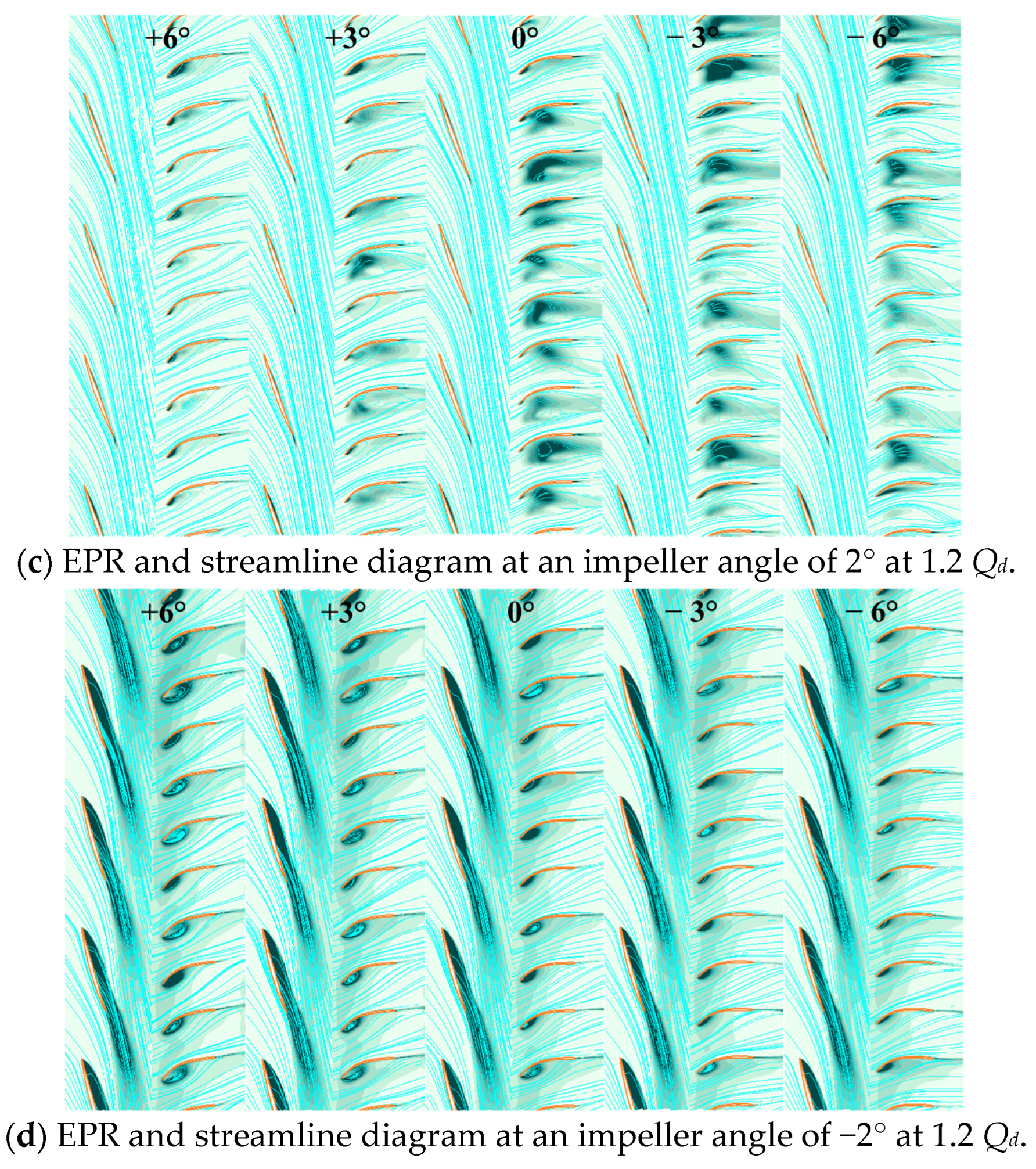
In the previous section, we analyzed the improvement in efficiency and the decrease in energy consumption after matching the moving and stationary blades. The efficiency improvement effect of using an adjustable guide vane is particularly significant under high-flow and low-flow conditions, and the adaptation of adjustable guide vanes varies with different impeller angles. In order to explore the internal flow patterns of the adjustable guide vane more clearly, we used the entropy production value method to analyze the local energy loss in the impeller and guide vane domains of the mixed-flow pump in this chapter, as well as to track its flow characteristics along with surface streamlines.

7.1. EPR Method

The formula for EPR is as follows:

$$S_{PD}={\displaystyle \frac{\mu }{\overline{T}}}\left[2\left\{{\left({\displaystyle \frac{\partial \overline{u}}{\partial x}}\right)}^2+{\left({\displaystyle \frac{\partial \overline{v}}{\partial y}}\right)}^2+{\left({\displaystyle \frac{\partial \overline{v}}{\partial z}}\right)}^2\right\}+{\left({\displaystyle \frac{\partial \overline{u}}{\partial y}}+{\displaystyle \frac{\partial \overline{v}}{\partial x}}\right)}^2+{\left({\displaystyle \frac{\partial \overline{u}}{\partial z}}+{\displaystyle \frac{\partial \overline{w}}{\partial x}}\right)}^2+{\left({\displaystyle \frac{\partial \overline{v}}{\partial z}}+{\displaystyle \frac{\partial \overline{v}}{\partial y}}\right)}^2\right]$$

(16)

$$S_{P{D}^{\prime }}={\displaystyle \frac{\mu }{\overline{T}}}\left[2\left\{\overline{{\left({\displaystyle \frac{\partial u^{\prime }}{\partial x}}\right)}^2}+\overline{{\left({\displaystyle \frac{\partial v^{\prime }}{\partial y}}\right)}^2}+\overline{{\left({\displaystyle \frac{\partial w^{\prime }}{\partial z}}\right)}^2}\right\}+\overline{{\left({\displaystyle \frac{\partial u^{\prime }}{\partial y}}+{\displaystyle \frac{\partial v^{\prime }}{\partial x}}\right)}^2}+\overline{{\left({\displaystyle \frac{\partial u^{\prime }}{\partial z}}+{\displaystyle \frac{\partial w^{\prime }}{\partial x}}\right)}^2}+\overline{{\left({\displaystyle \frac{\partial v^{\prime }}{\partial z}}+{\displaystyle \frac{\partial w^{\prime }}{\partial y}}\right)}^2}\right]$$

(17)

$$S_P=S_{P\overline{D}}+S_{P{D}^{\prime }}$$

(18)

$$\epsilon =S_{p}T{\displaystyle \frac{Q}{P}}\sqrt{{\displaystyle \frac{H}{g}}}$$

(19)

We input the formula for EPR into the CFD post to form a new parameter, then used this parameter to analyze the internal energy loss and flow characteristics of the impeller angle at 0.6 Q_d and 1.2 Q_d, which were 2° and −2°, respectively. We expanded the perspective to blade-to-blade, which is shown in the following figure.

7.2. Flow Field Analysis

According to the comparison between Figure 15a and Figure 15b, respectively, we can see that when the impeller angle was 2°, the angle of attack between the water flow and the impeller was very obvious, and there was significant energy loss in the area between adjacent impellers. When the impeller rotates at a positive angle, the guide vane should rotate from zero degrees to a positive angle to match the changes in the impeller (we discussed the angle issue in Section 2.2). Therefore, the best matching angle should be a positive-angle guide vane, and the worst should be a negative-angle guide vane. From Figure 15, it can be seen that the adjustment from −6° to +6° caused different positions of energy loss in the guide vane. At −6°, it can be seen that there was significant energy dissipation at the leading edge of the convex surface of the guide vane, and there were vortices caused by secondary flow in the guide vane channel, with significant energy loss at the edges of the vortices. The change in the −3° guide vane relative to the −6° one was that the position where energy dissipation occurred on the convex surface of the guide vane moved back a bit, causing the vortex clusters to contract and become smaller. When the angle of the guide vane was 0°, the position of energy loss on the convex surface occurred in the middle, and the vortex clusters no longer gathered but became sparse, reducing the phenomenon of channel blockage. When the angles of the guide vane were 3° and 6°, the energy loss on the convex surface of the guide vane continued to move backwards to the middle and rear parts, and the vortex clusters began to become sparse and develop to the trailing edge of the guide vane. It is worth noting that when the guide vane angle was 3°, the streamline between the impellers was very complex, resulting in collision and separation of the water flow. However, the highest efficiency values read from the post-processing were not +6°, but 78.83% of 0° and 78.30% of 6°, and the worst match was not −6°, but 77.39% of −3°. Under the working condition of 0.6 Q_d, it was observed that when the impeller angle was −2°, the angle of attack between the impeller and the water flow decreased, and the energy loss between the impellers was significantly reduced. The energy dissipation was concentrated on the working surface of the impeller. The energy loss in the area between the adjacent guide vanes was very small and mainly concentrated on the concave surface of the guide vane inlet, where a separation vortex was formed and energy dissipation was obvious. As the angle of the guide vane was adjusted from positive to negative, the vortex on the concave surface of the leading edge of the guide vane continuously decreased until it reached a minimum of −6°; The area of turbulent energy dissipation at the concave surface of the guide vane and the volume of the vortices also decreased continuously with the angle from positive to negative. At the same time, different angles of the guide vane imposed different constraints on the water flow. It can be clearly seen that during the rotation of the guide vane angle from positive to negative, the contact area between the trailing edge of the impeller and the concave surface of the guide vane decreased. At the concave surface of the 6° guide vane, it can be clearly seen that the shape of the guide vane constrained the flow of water, converting circumferential velocity into pressure energy. At the concave surface of the 6° guide vane, it can be seen that the guide vane did not have a strong constraint on the water flow, and the contact point between the water flow and the guide vane was more at the outlet edge of the latter.

As shown in Figure 15c,d, when the flow rate increased to 1.2 Q_d, the impeller angle was 2°. It can be clearly seen that the energy dissipation of the impeller working surface was significantly reduced, and the fit between the streamline and the impeller was also more appropriate. We can see that the energy dissipation at the concave surface of the 6° guide vane angle was only more significant at the inlet. As the guide vane angle changed towards a negative angle, the position of energy dissipation shifted towards the middle of the guide vane’s concave surface, and the area became larger. The combination with the highest efficiency was the −6° guide vane, and that with the lowest was the 6° guide vane. When the impeller angle was −2, there was still severe energy dissipation on the working surface of the impeller, and it can be seen from the streamline that there was a clear angle of attack between it and the impeller. From the concave surface of the 6° guide vane, it can be clearly seen that there was significant energy dissipation at the leading edge, and there were obvious vortices. As the guide vane angle was adjusted from positive to negative, the area of energy dissipation became smaller and the volume of vortices became smaller.

Through flow field analysis, we can see that the energy dissipation of the 2° impeller working surface was very significant at 0.6 Q_d. The higher the combined efficiency of energy dissipation at the guide vane, the more significant the energy dissipation at the 0° guide vane compared to the −6° guide vane. However, the former was 1.18% more efficient than the latter. Energy dissipation weakened at 1.2 Q_d: The higher the combined efficiency of energy dissipation at the guide vane, the more significant the energy dissipation at the −6° guide vane compared to the 6° guide vane. However, the former had efficiency 2.96% higher than the latter. The energy dissipation of the working surface of the 2° impeller was significant at 0.6 Q_d and 1.2 Q_d: at 0.6 Q_d, there was energy dissipation caused by vortices at the concave surface of the guide vane. The less obvious the combination efficiency, the higher the efficiency. The efficiency of the 6° guide vane was 1.13% higher than that of the −6° guide vane, and the same was true for 1.2 Q_d. The efficiency of the −6° guide vane with less obvious energy dissipation was 11.78% higher than that of the obvious 6° guide vane. This also indicates that the relationship between EPR value and efficiency changes with the change in the guide vane angle.

8. Conclusions

(1) The impeller is a key component necessary for the pump to perform work, and the angle of the adjustable impeller determines the shape of the efficiency curve and the position of the high-efficiency zone. The efficiency curve of the impeller’s positive angle adjustment moves towards a high flow rate, while the efficiency curve of the impeller’s negative angle adjustment moves towards a low flow rate. Positive-angle guide vanes are suitable for small-flow negative-angle impellers, while negative-angle guide vanes are suitable for large-flow positive-angle impellers. Adjustable guide vanes can only improve efficiency; they cannot change the shape of the efficiency curve. The use of adjustable guide vanes significantly improved efficiency, especially at the deviation from the design point. The greater the deviation from the design point, the more significant the improvement effect of the movable guide vane on efficiency was. The average increase in efficiency was 1.23% per operating point at an impeller angle of 2°, 0.5% per operating point at an impeller angle of 0°, and 2.99% per operating point at an impeller angle of −2°.

(2) The matching combination of moving and stationary blades with movable guide vanes is a key issue in vertical mixed-flow pumps. The use of movable guide vane significantly improves the efficiency of various operating conditions and suppresses the sharp increase in energy consumption during the transition process of extreme operating conditions. The energy consumption curve, which serves as the assessment indicator for pump stations, also experiences a significant decrease. However, with the improvement of efficiency, the head at the operating point will also change, and using the original pump station operation plan will cause energy waste. Therefore, for the management of pumping stations, it is necessary to develop a joint optimization and matching plan again in order to achieve the goal of reducing energy consumption and expanding the high-efficiency zone. The physical significance of the formula is presented at the guide vane.

(3) EPR can be effectively applied to flow field analysis. The flow analysis at the guide vane effectively demonstrates the effectiveness of EPR analysis. It reflects the relationship between changes in physical quantities such as speed and temperature, flow state, and energy loss. The entropy production rate not only represents the dissipation of energy, but also exhibits the characteristics of high EPR and high energy conversion efficiency (conversion from circumferential velocity to compressive energy and circumferential velocity at the guide vane). By marking the regions with high EPR, the changes in energy loss in the flow field can be clearly displayed when the matching of dynamic and static blades is poor. It guides the improvement design of turbomachinery, especially dynamic and static blade cascades.

References

1. Manivannan, A. Computational fluid dynamics analysis of a mixed flow pump impeller. Int. J. Eng. Sci. Technol. 2011, 30, 558–566. [Google Scholar] [CrossRef]
2. Li, W.; Ping, Y.; Shi, W.; Ji, L.; Li, E.; Ma, L. Research progress in rotating stall in mixed-flow pumps with guide vane. J. Drain. Irrig. Mach. Eng. 2019, 37, 737–745. [Google Scholar]
3. Kurokawa, J.; Jiang, J.; Kitahora, T. Inlet reverse-flow model and prediction of theoretical head and water power of mixed-flow pumps. JSME Int. J. Ser. B Fluids Therm. Eng. 1994, 37, 853–860. [Google Scholar] [CrossRef]
4. Kumar, A.; Hesheng, T.; Vashishtha, G.; Xiang, J. Noise subtraction and marginal enhanced square envelope spectrum (MESES) for the identification of bearing defects in centrifugal and axial pump. Mech. Syst. Signal Process. 2021, 165, 108366. [Google Scholar] [CrossRef]
5. Qian, Z.; Wang, Y.; Zheng, B.; Liu, D. Numerical simulation and analysis of performance of axial flow pump with adjustable guide vane. J. Hydroelectr. Eng. 2011, 30, 123. [Google Scholar]
6. Yang, F.; Liu, C.; Tang, F.; Zhou, J.; Cheng, L. Numerical Simulation on Hydraulic Performance of Axial-flow Pumping System with Adjustable Inlet Guide vane. Trans. Chin. Soc. Agric. Mach. 2014, 45, 51–58. [Google Scholar]
7. Al-Obaidi, A. Experimental Diagnostic of Cavitation Flow in the Centrifugal Pump Under Various Impeller Speeds Based on Acoustic Analysis Method. Arch. Acoust. 2023, 48, 159–170. [Google Scholar]
8. Kim, S.; Lee, K.-Y.; Kim, J.-H.; Kim, J.-H.; Jung, U.-H.; Choi, Y.-S. High performance hydraulic design techniques of mixed-flow pump impeller and diffuser. J. Mech. Sci. Technol. 2015, 29, 227–240. [Google Scholar] [CrossRef]
9. Tanaka, H. Vibration Behavior and Dynamic Stress of Runners of Very High Head Reversible Pump-turbines. Int. J. Fluid Mach. Syst. 2011, 4, 289–306. [Google Scholar] [CrossRef]
10. Jin, F.Y.; Tao, R.; Zhu, D.; Li, P.X.; Xiao, R.F.; Liu, W.C. Transient simulation of the rapid guide vane adjustment under constant head of pump turbine in pump mode. J. Energy Storage 2022, 56, 105960. [Google Scholar] [CrossRef]
11. Zhu, D.; Yan, W.; Guang, W.L.; Wang, Z.W.; Tao, R. Influence of Guide Vane Opening on the Runaway Stability of a Pump-Turbine Used for Hydropower and Ocean Power. J. Mar. Sci. Eng. 2023, 11, 1218. [Google Scholar] [CrossRef]
12. Tao, R.; Heng, Y.G.; Zhang, F.F.; Pan, J.L.; Zhu, D.; Liu, W.C.; Xiao, R.; Gui, Z. Analyzing the S-characteristic of pump-turbine under the same head condition from the perspective of flow energy dissipation. Proc. Inst. Mech. Eng. Part A: J. Power Energy 2023, 237, 1726–1742. [Google Scholar] [CrossRef]
13. Li, W.; Yang, Q.; Yang, Y.; Ji, L.; Shi, W.; Agarwal, R. Optimization of pump transient energy characteristics based on response surface optimization model and computational fluid dynamics. Appl. Energy 2024, 362, 123038. [Google Scholar] [CrossRef]
14. Belyaev, S.G.; Ishangaliev, T.S.; Kariev, D.A.; Kuklin, D.E. Energy investigations of a pumping station with an axial-flow pump and circular feed line. Hydrotech. Constr. 1991, 25, 683–685. [Google Scholar] [CrossRef]
15. Lu, J.; Chen, Q.; Liu, X.; Zhu, B.; Yuan, S. Investigation on pressure fluctuations induced by flow instabilities in a centrifugal pump. Ocean Eng. 2022, 258, 111805. [Google Scholar] [CrossRef]
16. Tao, R.; Wang, Z. Comparative numerical studies for the flow energy dissipation features in a pump-turbine in pump mode and turbine mode. J. Energy Storage 2021, 41, 102835. [Google Scholar] [CrossRef]
17. Qi, H.; Li, W.; Ji, L.; Liu, M.; Song, R.; Pan, Y.; Yang, Y. Performance optimization of centrifugal pump based on particle swarm optimization and entropy generation theory. Front. Energy Res. 2023, 10, 1094717. [Google Scholar] [CrossRef]
18. Al-Obaidi, A.R. Effect of Different Guide Vane Configurations on Flow Field Investigation and Performances of an Axial Pump Based on CFD Analysis and Vibration Investigation. Exp. Tech. 2024, 48, 69–88. [Google Scholar] [CrossRef]
19. Amiri, K.; Mulu, B.; Raisee Dehkordi, M.; Cervantes, M. Unsteady pressure measurements on the runner of a Kaplan turbine during load acceptance and load rejection. J. Hydraul. Res. 2015, 54, 56–73. [Google Scholar] [CrossRef]
20. Favrel, A.; Müller, A.; Landry, C.; Yamamoto, K.; Avellan, F. LDV survey of cavitation and resonance effect on the precessing vortex rope dynamics in the draft tube of Francis turbines. Exp. Fluids 2016, 57, 168. [Google Scholar] [CrossRef]
21. Olimstad, G.; Nielsen, T.; Børresen, B. Stability Limits of Reversible-Pump Turbines in Turbine Mode of Operation and Measurements of Unstable Characteristics. J. Fluids Eng. 2012, 134, 111202. [Google Scholar] [CrossRef]
22. Wang, C.; Wang, F.; An, D.; Yao, Z.; Xiao, R.; Lu, L.; He, C.; Zou, Z. A general alternate loading technique and its applications in the inverse designs of centrifugal and mixed-flow pump impeller. Sci. China Technol. Sci. 2021, 64, 898–918. [Google Scholar] [CrossRef]
23. Pope, S.B. The probability approach to the modelling of turbulent reacting flows. Combust. Flame 1976, 27, 299–312. [Google Scholar] [CrossRef]
24. Celik, I.; Ghia, U.; Roache, P.J.; Freitas, C.J. Procedure for Estimation and Reporting of Uncertainty Due to Discretization in CFD Applications. J. Fluids Eng. 2008, 130, 078001. [Google Scholar]
25. Guan, X. Morden Pumps Theory and Design; China Aerospace Publishing House: Beijing, China, 2011. [Google Scholar]
Figure 1. Schematic diagram of guide vane mixed-flow pump.
Water 17 00423 g001
Figure 2. Schematic diagram of adjustable guide vane rotation.
Water 17 00423 g002
Figure 3. Grid diagram.
Water 17 00423 g003
Figure 4. Grid independence verification.
Water 17 00423 g004
Figure 5. External characteristic curve.
Water 17 00423 g005
Figure 6. Three-factor k-avg value analysis.
Water 17 00423 g006
Figure 7. Flow efficiency curves at different impeller angles.
Water 17 00423 g007
Figure 8. Three-factor k-avg value analysis.
Water 17 00423 g008
Figure 9. Schematic diagram of matching dynamic and static blades.
Water 17 00423 g009
Figure 10. Efficiency curves of matching dynamic and static blades under different operating conditions.
Water 17 00423 g010aWater 17 00423 g010b
Figure 11. Efficiency diagram of matching impeller angles with adjustable guide vanes.
Water 17 00423 g011
Figure 12. Comparison of efficiency curves between adjustable guide vane and fixed guide vane.
Water 17 00423 g012
Figure 13. Efficiency curve envelope after adjusting the angle of the adjustable guide vane and fixed guide vane impeller.
Water 17 00423 g013
Figure 14. Energy consumption comparison chart.
Water 17 00423 g014
Figure 15. Entropy production value and streamline.
Water 17 00423 g015aWater 17 00423 g015b