Abstract
This research explores the distribution, transport, and deposition of calcium carbonate particles in the colorful pools of the Huanglong area under varying hydrodynamic conditions. The study employs Particle Image Velocimetry (PIV) for real-time measurements of flow field velocity and computational fluid dynamics (CFD) simulations to analyze particle behavior. The findings reveal that under horizontal flow conditions, the peak concentration of calcium carbonate escalated to 1.06%, representing a 6% surge compared to the inlet concentration. Significantly, particle aggregation and settling were predominantly noted at the bottom right of the flow channel, where the flow boundary layer is most pronounced. In the context of inclined surfaces equipped with a baffle, a substantial rise in calcium carbonate concentrations was detected at the channel’s bottom right and behind the baffle, particularly in regions characterized by reduced flow velocities. These low-velocity areas, along with the interaction of the boundary layer and low-speed vortices, led to a decrease in particle velocities, thereby enhancing deposition. The highest concentrations of calcium carbonate particles were found in regions characterized by thicker boundary layers, particularly in locations before and after the baffle. Using the Discrete Phase Model (DPM 22), the study tracked the trajectories of 2424 particles, of which 2415 exited the computational channel and nine underwent deposition. The overall deposition rate was measured at 0.371%, with calcium carbonate deposition rates ranging from 4.06 mm/a to 81.7 mm/a, closely matching field observations. These findings provide valuable insights into the dynamics of particle transport in aquatic environments and elucidate the factors influencing sedimentation processes.
1. Introduction
Travertine deposits are formed by the primary precipitation of freshwater carbonates and are distributed worldwide [1]. Research on travertine deposits mainly focuses on morphology, mineralogy, and isotope analysis. Based on geomorphology and depositional environment, the main forms of travertine deposits can be classified as follows [2,3,4,5]: terraced pools, stream flows, waterfalls, lakes, and caves. Morphological variations in travertine may be caused by different travertine deposition patterns [6], and erosion may alter their morphology [7,8]. The minerals that make up these different types of travertine provide a sensitive environmental record of water chemistry, hydrological transport, and climate [9]. The Huanglong landscape water is a special multi-phase fluid involving solid, liquid, and gas phases [10,11], mainly composed of CaCO3 particles formed by strong degassing of saturated CO2 in karst water rich in Ca2+, water, and free CO2 in water. It is significant to understand the growth mechanism of travertine landscape in order to analyze the deposition process of calcium carbonate by scientific means and identify the stacking mode of travertine particles. Özkul et al. [12] pointed out that the main mineral components of travertine deposits are calcite and aragonite, both of which are highly sensitive to hydrodynamic conditions. Different hydrodynamic factors such as flow rate and pressure respond to varying degrees based on geological conditions, and these differentiated geological conditions can lead to the formation of various forms of travertine landscapes.
Computational Fluid Dynamics (CFD) is a multidisciplinary numerical simulation technique that has demonstrated exceptional versatility and practical value across a wide range of industries. By solving the partial differential equations governing fluid flow and heat transfer, CFD enables the precise simulation of complex fluid dynamics, heat transfer, and multiphysics coupling phenomena. Its broad applicability spans industries such as aerospace, chemical engineering, automotive and marine, energy, mining and metallurgy, hydropower, agriculture, architecture, environmental protection, and biomedical sciences. In the chemical industry, CFD finds extensive applications in reactor design, flow mixing optimization, and multiphase flow simulations. Typical uses include modeling fluid flow within chemical reactors, studying gas–liquid mass transfer phenomena, and predicting particle flow behavior to enhance production efficiency [13]. In mining and metallurgy, CFD is utilized for mineral processing, ventilation system design, and molten metal flow studies. For instance, CFD optimizes flow in blast furnaces, improving smelting efficiency and product quality [14]. CFD plays a significant role in hydropower engineering, where it is used to analyze river flow dynamics, spillway discharge patterns, and turbine flow characteristics. This helps optimize hydraulic structure designs, ensuring safety and efficiency in hydropower projects [15].
This study transiently records the flow field velocity distribution of the source water at the Huanglong Wucai Pools using Particle Image Velocimetry (PIV) and conducts computational fluid dynamics simulations using Ansys Fluent 19. By analyzing the velocity distribution information at numerous spatial points, the spatial structure of the flow field and flow characteristics are obtained. At the same time, the flow field distribution and velocity vector distribution under different working conditions are calculated, thereby understanding the deposition of calcium carbonate in the gas–water–rock three-phase flow, providing a scientific theoretical basis for the travertine particle deposition process.
2. Research Methods
2.1. Analysis Method
The field flow velocity was measured using a handheld radar velocimeter (Decatur SVR-3D), and the transient flow characteristics were captured using a 2D PIV (Particle Image Velocimetry) system(Table 1). Samples were collected and stored at a low temperature of 0–4 °C to ensure their stability. Combined with the hydrogeological conditions of the study area, CFD was used to simulate the transport and distribution of calcareous particles in the water, with Ansys Fluent 19 employed to solve the interaction between the moving fluid and the solid surface.

Table 1.
Main experimental devices and related equipment.
2.2. Model Construction
CFD models were used for the numerical simulation of the flow boundary layer in the Huanglong area’s water source. Since the CFD method can obtain detailed information about the flow field, and with its DPM introduced in recent years, CFD technology has been widely used in the field of particle flow calculations. Although the underlying theory of CFD is not yet fully mature and computational results need experimental verification, it is undeniable that the CFD method is currently the most widely used and ideal tool for predicting fluid flow field distribution. CFD was used to simulate the transport and distribution of particles in terraced pools [16,17,18,19], with the continuous phase modeled using the RNG k-ε model, and the particle phase modeled using the Discrete Phase Model (DPM). The particle volume fraction was kept below 10%, and particle interactions were not considered [20,21,22,23,24,25,26].
The deposition process of calcium carbonate is a complex natural phenomenon, and it is impractical to analyze its entire process using a single model. Therefore, this paper employs three models to calculate the deposition process. The Eulerian model is used to calculate the variation trend of calcium carbonate particles in water, the VOF model is used to calculate the boundary layer distribution of water flow under the action of the riverbed and air, and the DPM is used to predict the trajectory of calcium carbonate particles in water. Based on this, this paper designs 5 cases, and the specific model selection is shown in Table 2.
Table 2.
The model selected for this simulation.
(1) Physical Model. The water source in the Huanglong region courses through a channel, carrying a significant concentration of calcium carbonate particles. Initially, the calcium carbonate in the water is not visible to the naked eye. After one week of flow, significant calcium carbonate deposits can be observed on the channel walls. The calcium carbonate content in the water ranges from approximately 0.001% to 0.01%, with over 95% of the Huanglong particles having diameters in the range of 1–5 μm (averaging around 3 μm), and particle viscosity ranging from 300 to 350 mPa·s.
(2) Computational Theory and Methods.
Transport Equations: During fluid flow, physical laws must be adhered to, specifically the three major laws of conservation: mass, momentum, and energy. When described mathematically, these correspond to the continuity equation, the momentum conservation equation, and the energy conservation equation, respectively.
Continuity Equation: This equation represents the law of mass conservation that fluid follows during the flow process. It can be expressed as: the increase in mass within a fluid element over a unit of time is equal to the net mass inflow into that element over the same time interval [27,28]. Mathematically, it is expressed as:
In the equation, Sm represents the mass source term per unit volume, and ρ represents the fluid density; typically, Sm is zero.
Momentum Conservation Equation: Essentially Newton’s second law, it can be stated as follows: the rate of change in momentum of the fluid in an element over time is equal to the sum of all forces acting on that element [29,30]. Mathematically, it is expressed as:
In the equation, μ represents the molecular viscosity, and I is the unit tensor.
Turbulence Model—k-ε Model: Based on the Reynolds number, fluid flow can be classified as either laminar or turbulent [31,32]. Although indoor airflow typically falls within the range of low-speed flow, it generally remains in a turbulent state, so the turbulence model is used for three-dimensional, unsteady, and incompressible numerical simulation of indoor airflow.
For a turbulent flow field, the ideal approach is to ensure that all temporal and spatial scales are resolved down to the Kolmogorov scale; this method is known as Direct Numerical Simulation (DNS). While DNS can directly solve the transient flow field, the computational cost is too high, making it impractical for many engineering applications. Instead, the Reynolds-averaged models are often used, which focus on the time-averaged characteristics of the flow and neglect the details of turbulence. As such, most engineering turbulence calculations still rely on Reynolds-averaged equations, such as the k-ε and k-ω models. Based on this, the widely used k-ε model will be adopted.
Turbulent Kinetic Energy (k) Equation:
In the k equation, from left to right, the terms represent the time variation term, convection term, diffusion term, shear production term, buoyancy production term, and turbulent dissipation term.
Turbulent Dissipation (ε) Equation:
In the equation, μT is the turbulent viscosity coefficient. c1ε, c1ε, c1ε are constants, while σk and σε represent the turbulent Prandtl numbers for k and ε, respectively.
When calculating the flow of water in open channels (with air above the water), a three-phase flow involving gas (air), liquid (water), and solid (calcium carbonate particles) actually occurs. The Eulerian model is used to predict the deposition trend of calcium carbonate [33,34]. To study the motion of particles within the fluid, the discrete phase model is employed.
In addition, different cases require different multiphase flow models:
In the Lagrangian coordinate system, when the continuous phase is fluid and the carried phase consists of solid particles, the mechanical equilibrium equation for the particles is given by:
F represents the pressure gradient and body forces acting on a unit particle; FD (u − up) is the drag force per unit mass on the particle, where
In the equation: u is the fluid velocity, up is the velocity of the solid phase particle, ρp is the density of the solid phase particle, Dp is the diameter of the solid phase particle, CD is the drag coefficient, Re is the relative Reynolds number of the fluid.
Eulerian Model: The portrayal of multiphase flow as interpenetrating continua embraces the notion of phasic volume fractions, denoted in this context by αq. These volume fractions signify the proportion of space inhabited by each phase, with the principles of mass and momentum conservation being independently upheld by each phase. The volume of phase q, Vq is defined by
where
The continuity equation for phase q is
In the equation, mqp represents the mass transfer from phase q to phase p, while mqp denotes the mass transfer from phase p to phase q. In the default case, the right side of the equation is set to Sq = 0 but can specify a constant or user-defined mass source for each phase.
Volume of Fluid (VOF) Model: The VOF model simulates two or more immiscible fluids by solving separate momentum equations and tracking the volume fraction of each fluid throughout the region.
Volume Fraction Equation: The interface between phases is tracked by solving the continuity equation for the volume fraction of a single phase or multiple phases. For the qqq-th phase, this equation is expressed as follows:
In the equation, mqp represents the mass transfer from phase q to phase p, while mqp denotes the mass transfer from phase p to phase q. In the default case, the right side of the equation is set to sαq = 0, but a constant or a customized mass source can be specified for the inter-phase transfer.
The calculation of the primary phase volume fraction is based on the following constraints:
The volume fraction equation can be solved using implicit or explicit time discretization methods.
(3) Parameter Configuration. The simulation employs Ansys Fluent 19 as the computational solver. ① Boundary Condition: Within this model, the medium inlet is configured as a velocity inlet, the medium outlet as a pressure outlet, and the channel’s bottom boundary is designated as a no-slip wall. ② Average Velocity Inlet: The typical velocity of water at the Huanglong landscape is within the range of 1–2 m/s. For the purposes of this calculation, an inlet flow velocity of 1 m/s has been selected. ③ Residual Settings: The convergence criterion for the energy equation is conventionally set to 1 × 10⁻⁶, whereas for the flow equation, it is generally set to 1 × 10⁻⁵. These convergence criteria are indicative of the simulation results’ precision. The convergence status can be tracked through the monitoring window, with optimal convergence indicated by a residual graph that trends towards a horizontal line. ④ Time Step: Given that this calculation pertains to an unsteady and turbulent flow field, it necessitates the specification of a time step. The time step corresponds to the physical time associated with each computational step. For an unsteady flow field, it is approached as a sequence of quasi-steady flow fields, with each time step representing the duration for each quasi-steady state. In this simulation, the time steps are set to 0.001 s and 0.004 s, with corresponding Courant Numbers of 2 and 8. While smaller time steps provide enhanced accuracy, they also prolong the computation time. To safeguard the reliability of the computational outcomes, the Courant Number is advised not to surpass 10. Owing to the significant computational demands, the initial concentration of calcium carbonate has been scaled up to expedite the computation process.
2.3. Density Variations in CFD Simulations
Calcium carbonate particles with different formulations may exhibit variations in density, particle size, and shape, which influence their sedimentation velocity, distribution, and interactions with the water body. For example, during dissolution (CaCO3→Ca2++CO32−) or precipitation (Ca2++CO32−→CaCO3↓), the mass and volume of calcium carbonate particles change, affecting their density and volume concentration. When dissolved salts in water (e.g., changes in Ca2+ concentration) or temperature distribution is uneven, the fluid density also changes, which in turn affects the distribution of the particles.
(1) Multiphase Flow Extension
① Euler–Euler Model: This model introduces the density and concentration of the particle phase (solid phase) to simulate the coupling between the particle phase and the fluid phase. Particle density can be set as a function of time or location to reflect the dynamic changes due to the dissolution or precipitation of calcium carbonate.
② Euler–Lagrange Model: In this model, particle density is treated as an attribute that updates over time, allowing the CFD program to track the sedimentation paths of individual particles in real time.
(2) Kinetic Coupling of Density Changes
If density variations are caused by chemical reactions (e.g., dissolution or precipitation), a kinetic model of the chemical reactions needs to be incorporated. For instance:
① Mass Conservation Coupling. The solute concentration (e.g., Ca2+ and CO32−) is coupled into the mass conservation equation:
where C is the solute concentration, and R is the reaction rate.
② Mass Transfer Model. This describes the dissolution or precipitation process between the particles and the fluid. The mass transfer rate can be expressed as:
where kA is the mass transfer coefficient, Csat is the saturation concentration, and Cbulk is the solute concentration at the particle surface.
(3) Spatial Variations in Fluid Density
If fluid density is non-uniformly distributed (e.g., due to temperature or solute concentration gradients), CFD fluid properties can be set to define density as a function of space or temperature:
where β is the coefficient of thermal expansion, and T is the temperature.
2.4. Boundary Layer Analysis
In CFD, the analysis of the boundary layer is a critical step in accurately simulating fluid flow, heat transfer, and phenomena near solid surfaces. The boundary layer refers to the region near a solid surface where velocity gradients develop due to viscous effects. Boundary layer analysis primarily involves mesh generation, turbulence modeling, and the setup of boundary conditions. The analysis of boundary layers is a critical component in understanding the behavior of fluid flow near solid surfaces. The boundary layer is the thin region of fluid where viscous effects are significant, and it plays a key role in determining drag, heat transfer, and flow separation in many engineering applications. CFD provides a detailed framework for studying the boundary layer by solving the governing Navier–Stokes equations along with appropriate boundary conditions. Here is how boundary layers are typically considered in CFD analysis:
(1) Defining Boundary Conditions. To model the boundary layer accurately, appropriate boundary conditions must be set at the surface of the solid object (e.g., a wing, pipe wall, or cylinder). The most common boundary conditions are:
① No-slip Condition. The velocity of the fluid at the wall is assumed to be zero in the reference frame of the solid boundary. This condition is crucial because it defines the velocity profile within the boundary layer.
② Wall Shear Stress. In addition to velocity, wall shear stress (tangential force per unit area) is an important quantity, especially in turbulent flows. CFD models calculate this stress based on the flow velocity gradient at the wall.
(2) Meshing the Boundary Layer. CFD models rely on computational grids (meshes) to discretize the fluid domain. To accurately capture the boundary layer, a fine mesh must be applied near the wall where the flow undergoes rapid changes in velocity and turbulence. A common technique is to use boundary layer meshes that are refined in the near-wall region. These meshes are typically structured with layers of cells oriented normally to the wall, with the first cell placed close to the wall. This ensures that the velocity gradient in the boundary layer is resolved with sufficient accuracy. One of the key parameters in boundary layer meshing is the Y+ value, which represents the distance of the first grid cell from the wall in wall units. The choice of Y+ influences the turbulence model used (e.g., for Y+ < 5, a wall function approach is often used, while for Y+ > 30, near-wall turbulence models may be necessary).
(3) Turbulence Modeling. In the boundary layer, turbulence can have a significant effect on the flow characteristics, especially in high Reynolds number flows. CFD simulations must account for turbulence using appropriate models. Common approaches include: ① RANS (Reynolds-Averaged Navier–Stokes) models. These models average the effects of turbulent fluctuations, with specific turbulence models (e.g., k-ε, k-ω, or SST models) providing closure for the equations. In boundary layer analysis, these models are often used in conjunction with near-wall treatment methods like wall functions or low-Reynolds-number models. ② LES (Large Eddy Simulation) and DNS (Direct Numerical Simulation). For more accurate results, especially in complex flows with separation, LES and DNS can be used. However, they are computationally expensive and generally applied in more research-oriented simulations rather than routine engineering analysis.
(4) Velocity and Temperature Profiles. The boundary layer typically exhibits a steep velocity gradient near the wall. CFD simulations can provide detailed profiles of velocity, temperature, and other fluid properties across the boundary layer. These profiles reveal: ① Laminar Boundary Layers: In low Reynolds number flows, the boundary layer may remain laminar, characterized by smooth and orderly flow. CFD simulations can capture the velocity gradient and the transition to turbulence. ② Turbulent Boundary Layers: In high Reynolds number flows, the boundary layer may become turbulent, leading to significant mixing and increased friction. CFD models predict the onset of turbulence and the development of turbulent structures in the boundary layer. ③ Heat transfer in the boundary layer: For conjugate heat transfer problems, CFD can predict the temperature gradients within the boundary layer, helping to optimize thermal management in applications like heat exchangers or aerodynamic surfaces.
(5) Flow Separation and Transition. The boundary layer is crucial in understanding flow separation, which occurs when the fluid in the boundary layer cannot stay attached to the surface due to adverse pressure gradients. CFD simulations can track the development of the boundary layer, predict when and where separation will occur, and help in designing surfaces that minimize separation (e.g., using boundary layer control techniques like vortex generators). In addition, CFD can predict the transition from laminar to turbulent flow in the boundary layer, which is an important aspect in many practical applications (such as aircraft wing design). This transition is influenced by factors like surface roughness, pressure gradients, and freestream turbulence, all of which can be modeled using CFD of ANSYS Fluent.
(6) Wall Functions and Near-Wall Treatment. For turbulent flow, especially in high Reynolds number cases, it is common to use wall functions to approximate the near-wall behavior without resolving the smallest scales of turbulence. These wall functions are based on empirical correlations and are typically used in RANS models to avoid the need for extremely fine meshes near the wall. However, for more accurate results, especially in regions with high turbulence, advanced near-wall turbulence models like low-Reynolds-number models may be employed to resolve the full boundary layer.
(7) Validation and Comparison. Once the boundary layer has been modeled in CFD, it is important to validate the results with experimental data or analytical solutions. This includes comparing velocity profiles, shear stress distributions, and heat transfer rates with known benchmarks or wind tunnel data. Validation ensures that the CFD model is accurately capturing the physics of the boundary layer and can be reliably used for design purposes.
3. Results and Discussion
Depending on the research object, this calculation is divided into three flow situations: ① horizontal flow field; ② inclined flow field; ③ boundary layer of the inclined flow field set by the discrete phase model. In the first two conditions, the air above the water flow is free flowing, while in the latter two conditions, a baffle is present on the right side of the inlet. The bottom of the flow region can be simplified to a wall, and wall thickness can be neglected.
3.1. Horizontal Flow Field Travertine Deposition Process
This section of the calculation employs a horizontal flow method, utilizing the source water from the colorful pond in the Huanglong Scenic Area. Since this calculation focuses on the boundary layer formed between the flowing Huanglong water source and the bottom channel, the model can be simplified to a 2D plane. The inlet flow velocity is set at 1 m/s, with a water height of 30 mm (H1). Above the flow field is air (H2 = 70 mm), with the fluid entering from the left side and exiting on the right. The computational domain is shown in Figure 1, measuring 1000 mm in length (L). The total number of grid elements is 65,000, and the minimum height of the mesh is 1 mm in the H1. The density of water is 998.2 kg/m3, and its viscosity is 0.001003 kg/(m·s); the density of calcium carbonate is 2800 kg/m3, with a viscosity of 1.75 × 10⁻5 kg/(m·s), and the particle diameter is 5 × 10⁻6 m, with a concentration of 1%.
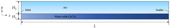
Figure 1.
Calculation domain of horizontal flow field.
Figure 2 shows the velocity contour of the water flow, the distribution of calcium carbonate particles, and their corresponding velocity contours under these operating conditions. Due to limited calculation time, the flow duration is short, and the results are expressed in terms of the aggregation degree of calcium carbonate to illustrate its deposition trend and deposition locations.
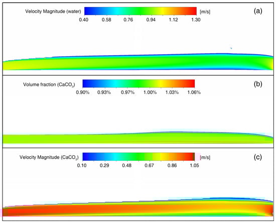
Figure 2.
Horizontal flow field: (a) velocity cloud image, (b) CaCO3 distribution, (c) CaCO3 velocity cloud image.
From Figure 2a, it can be observed that after the water flows in from the left inlet, the flow height increases compared to the initial 30 mm due to the presence of air above it. At the bottom, the water flow velocity is zero, resulting in the formation of a flow boundary layer. As the flow develops, the boundary layer begins to thicken on the right side. According to the simulation calculations, the maximum concentration of calcium carbonate reaches 1.06%, which is an increase of 6% compared to the inlet.
As shown in Figure 2b, there is a significant increase in calcium carbonate concentration at the bottom right side of the flow. This location corresponds to the thickest part of the flow boundary layer, where calcium carbonate particles have aggregated and settled. Figure 2c displays the velocity contour of the calcium carbonate particles. Due to the presence of the boundary layer, the particles experience a reduction in speed as they flow, ultimately creating a low-speed area at the bottom right. With the decrease in particle flow velocity, the deposition of calcium carbonate occurs.
3.2. Inclined Plane Flow Field Travertine Deposition Process
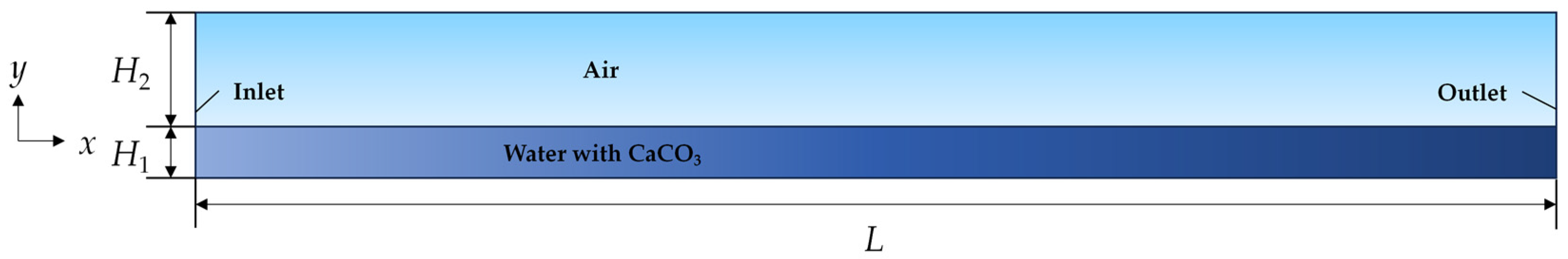
In the inclined flow field condition for calcite deposition, water flows down a slope, with a baffle located on the right side of the water inlet (L1 = 30 mm). The water source from the Huanglong area (containing 1% CaCO3) has an inlet flow velocity of 1 m/s and a flow height of 30 mm (H1). Above the flow field is air (H2 = 270 mm), with the fluid entering from the left and exiting on the right. The computational domain is illustrated in Figure 3, measuring 300 mm in length and 300 mm in height, with the slope having a height of 30 mm (H3). The total number of grids is 214,368, and the minimum height of the mesh is 0.5 mm in the H1.

Figure 3.
Calculation domain of the inclined plane flow field.
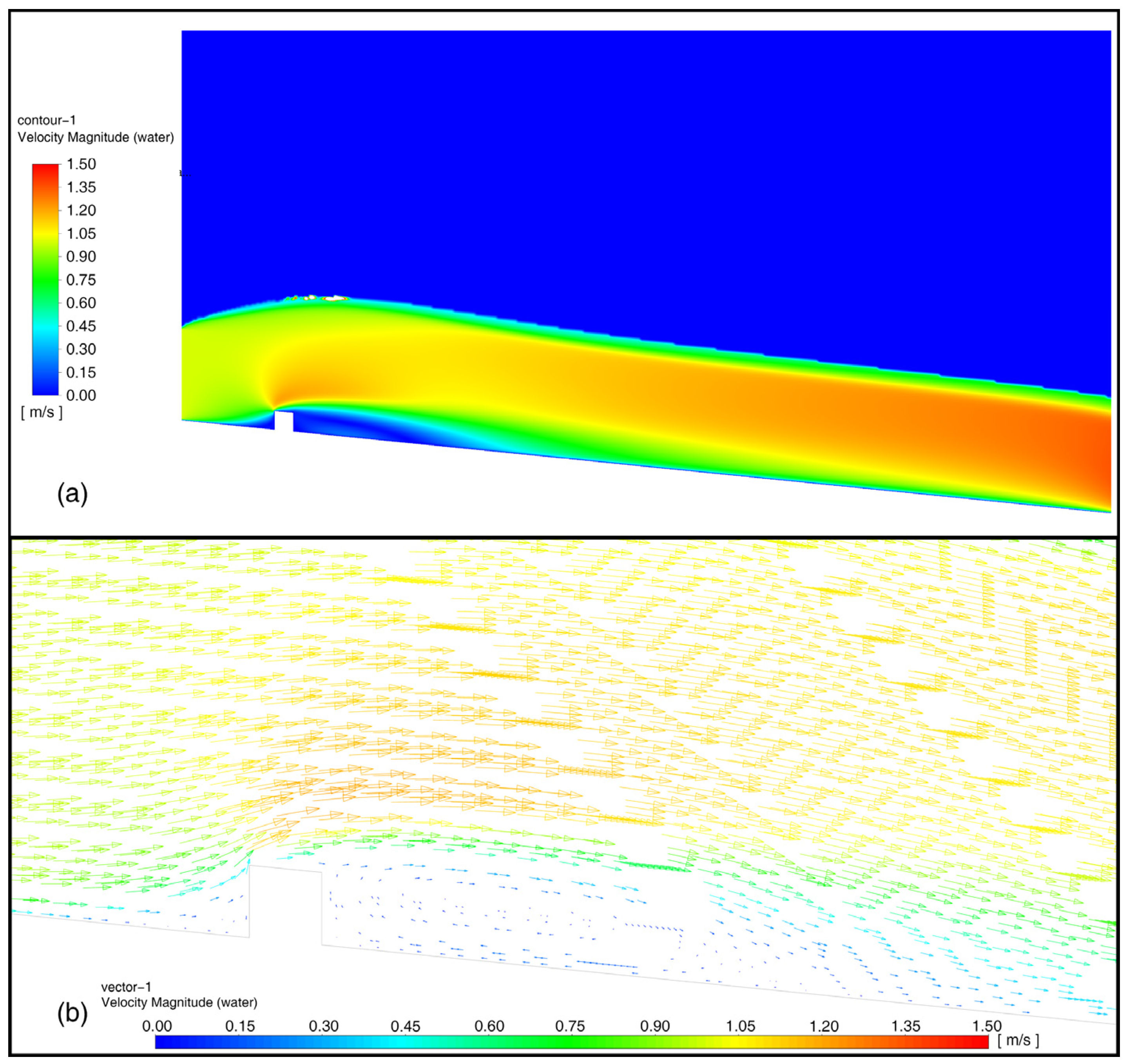
Figure 4 displays the velocity contour map and velocity vector diagram of the water flow under the inclined flow field condition.

Figure 4.
Velocity distribution of inclined plane flow field: (a) velocity cloud image, (b) velocity vector image.
From Figure 4a, it can be seen that when water flows in from the left side and encounters the baffle, it begins to flow around it, creating a low-speed vortex area behind the baffle. A stable boundary layer also forms at the bottom right side. The velocity vector diagram is shown in Figure 4b. Based on the results from the horizontal flow field, it can be predicted that calcium carbonate particles will accumulate in the low-speed vortex area behind the baffle and at the bottom right side.
Figure 5 illustrates the distribution and velocity of calcium carbonate in the inclined flow field of water.
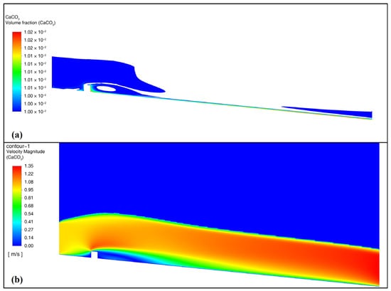
Figure 5.
Inclined plane flow field CaCO3 particles: (a) distribution, (b) velocity cloud image.
By adjusting the display range to only observe areas where the concentration of calcium carbonate particles is greater than or equal to 1%, Figure 5a shows that there is a significant increase in calcium carbonate concentration at the bottom right side of the water flow and behind the baffle. Comparing this with Figure 4a, it can be noted that these locations correspond to areas of reduced flow velocity, where calcium carbonate particles accumulate and settle in the low-velocity zones.
Figure 5b presents the velocity cloud diagram of the calcium carbonate particles. Due to the presence of the boundary layer and the low-speed vortex area, the particles experience a decrease in velocity as they flow through, ultimately resulting in the formation of a low-speed zone behind the baffle and at the bottom right side. As the flow speed of the particles decreases, the deposition of calcium carbonate occurs progressively.
3.3. Boundary Layer Effect of Inclined Plane Flow Field
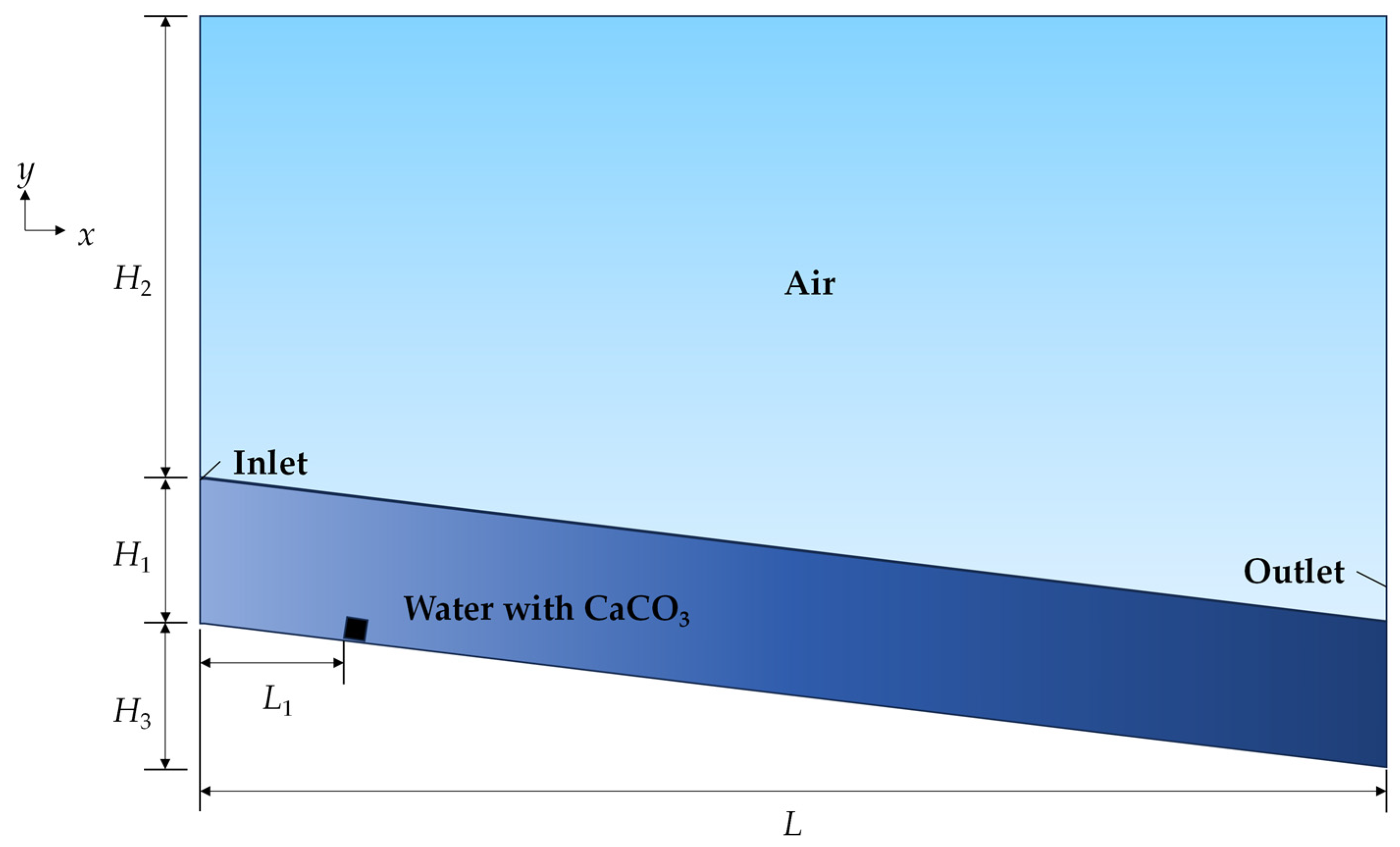
The boundary layer effect in the sloped flow field involves water flowing over a slope with a baffle located to the right of the water inlet (L1 = 50 mm). The water source in the Huanglong region, containing 1% CaCO3, has an inlet flow velocity of 1 m/s, and the flow height is 30 mm, with fluid entering from the left side and exiting on the right side. The computational domain is illustrated in Figure 6, measuring 500 mm in length (L) and 30 mm in height (H1), with a slope height of 30 mm (H2). The total mesh count is 1,773,853, and the minimum height of the mesh is 0.05 mm in the H1.
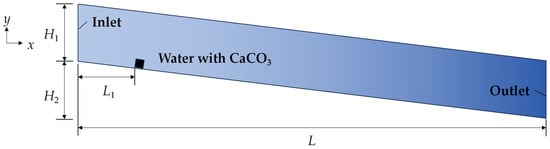
Figure 6.
Calculation domain of boundary layer effect condition of the inclined plane flow field.
To predict the movement trajectories of particles in the fluid, the Discrete Phase Model (DPM) is employed for the calculations. In the particle force balance, additional forces are considered, as indicated in Formula (10) (F): one is the virtual mass force, which is the force required to accelerate the surrounding fluid, and the other is the Saffman [35] lift force, which arises from the lateral velocity gradient (shear layer flow). The virtual mass force can be expressed. The lift on small sphere in flow.
In the equation, the virtual mass force factor Cvm has a default value of 0.5, K = 2.594, and dij represents the fluid deformation rate tensor. This consideration is crucial when dealing with submicron-sized particles (with diameters ranging from 1 to 10 μm), as it accounts for the effects of fluid dynamics on the motion of such small particles.
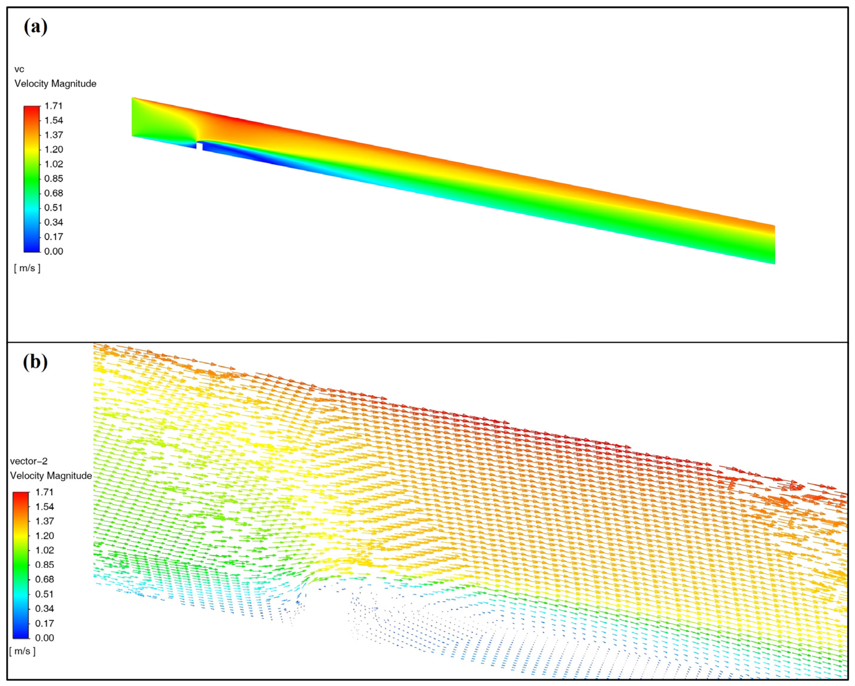
Figure 7 shows the velocity contour and velocity vector diagrams of the water flow under this condition.

Figure 7.
(a) Velocity cloud image of water flow, (b) velocity vector image of water flow.
From Figure 7a, it can be seen that the maximum water flow velocity is 1.708 m/s, represented in deep red, while the minimum velocity is 0 m/s, distributed around the front and rear of the baffle and along the wall at the bottom of the flow channel. As shown in Figure 7b, when the water flows in from the left side and encounters the baffle, it begins to flow around it, creating a low-speed vortex zone behind the baffle, as well as forming another stable boundary layer at the bottom right. Based on the calculations from previous conditions, it can be predicted that calcium carbonate particles will accumulate in the low-speed vortex zone behind the baffle and at the bottom right.
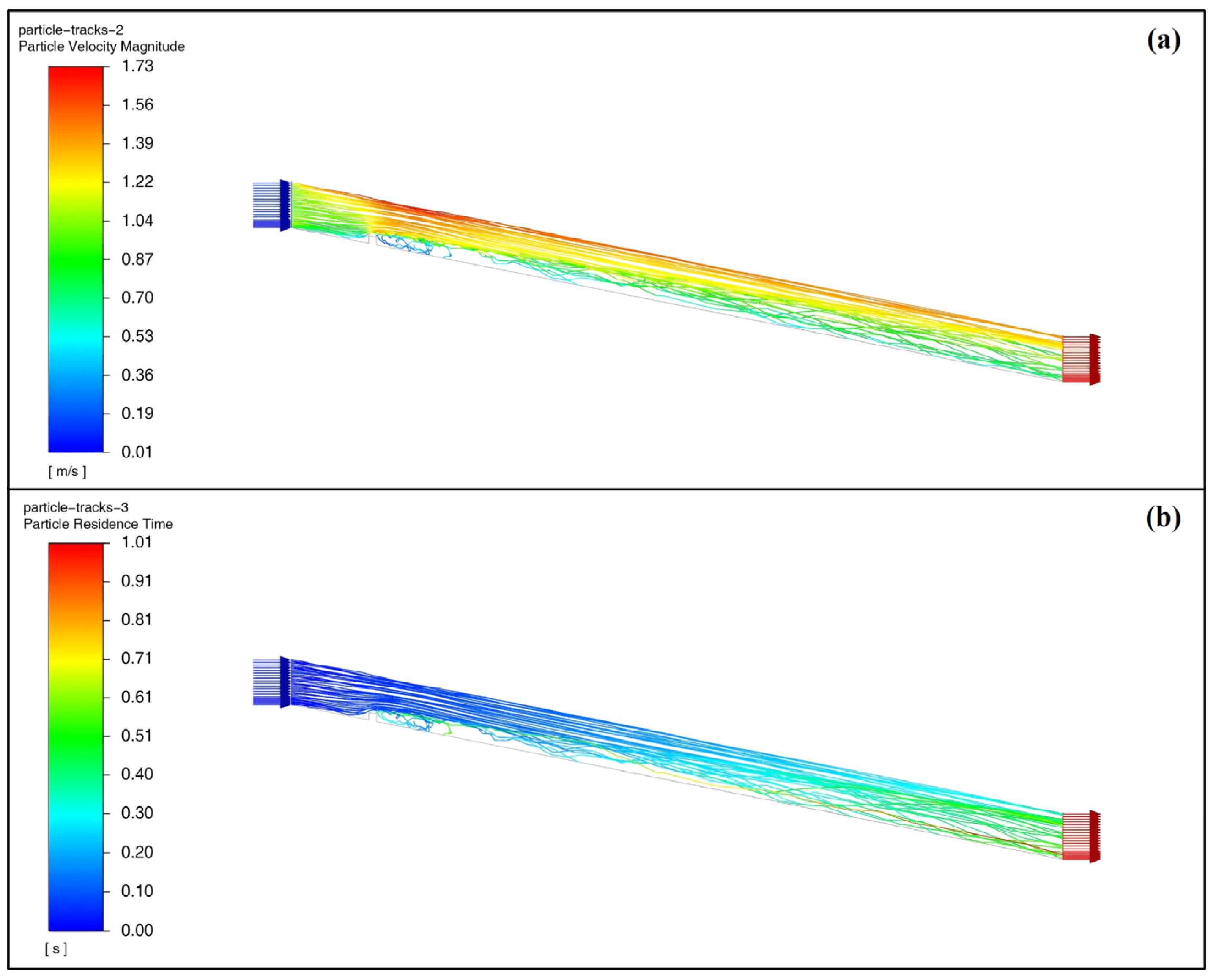
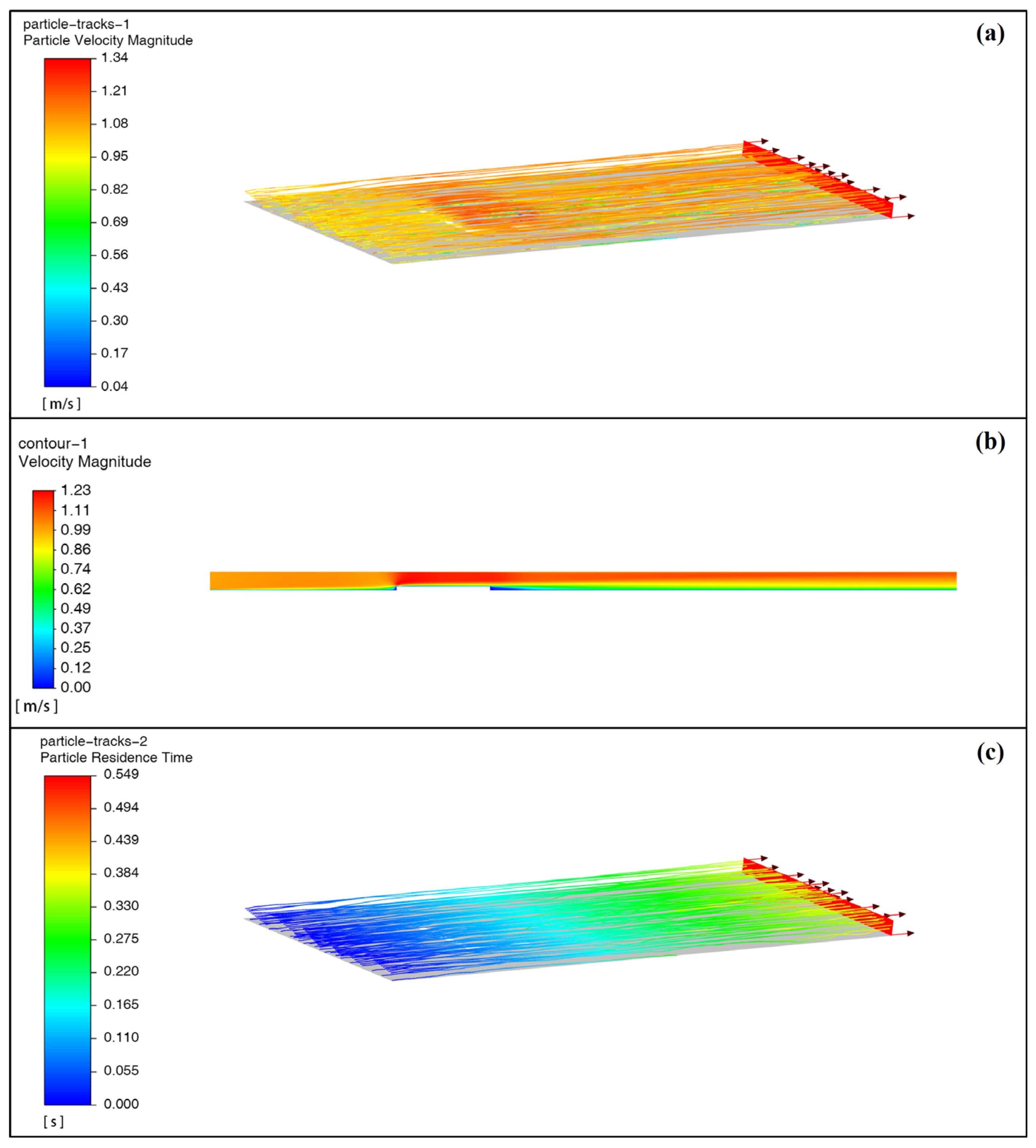
Figure 8 illustrates the movement trajectories and residence times of the calcium carbonate under these conditions.
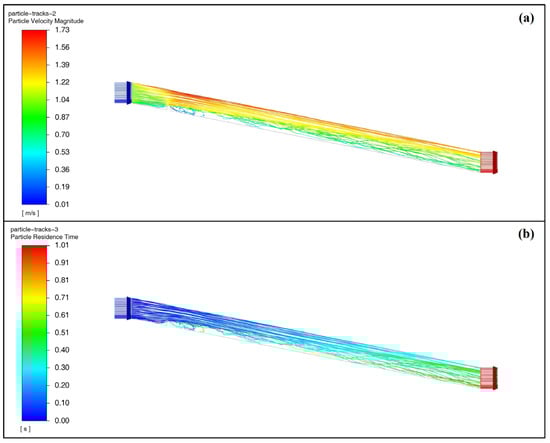
Figure 8.
(a) Trajectory velocity of CaCO3 in water, and (b) cloud image of flow velocity of CaCO3 particles.
Figure 8a displays the movement trajectories of calcium carbonate particles in water, with colors representing the velocities of the fluid particles. Comparing this with Figure 7a, it can be observed that the velocity of the particles is influenced by the velocity of the fluid in their respective locations—i.e., the faster the fluid velocity, the faster the particle velocity, and vice versa. The particles that experience slower velocities are primarily concentrated within the boundary layer, where they are more likely to be captured by the bottom of the flow channel and thus undergo deposition. Areas of particle deposition include not only the downstream section of the channel but also the vortex region adjacent to the baffle.
Adjusting the displayed colors to represent particle residence times yields Figure 8b. If the particles do not experience deceleration, their transit time through the channel is 0.50 s, with most particles exiting the channel having a residence time between 0.40 and 0.60 s.
In light of the deposition situations in Conditions 3.1 and 3.2, the distribution of the boundary layer under these flow conditions was computed separately. Since the focus is more on the movement relationship between the water and air phases, the VOF model was employed for the simulation, with the water–air distribution shown in Figure 9.
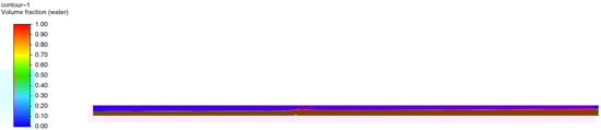
Figure 9.
Water and air distribution.
The computational model consists of a channel that is 1 m long, with a rectangular baffle measuring 2 mm on each side positioned 0.4 m from the right side of the inlet. The water surface height is 8 mm, and the area above the water surface is filled with freely flowing air.
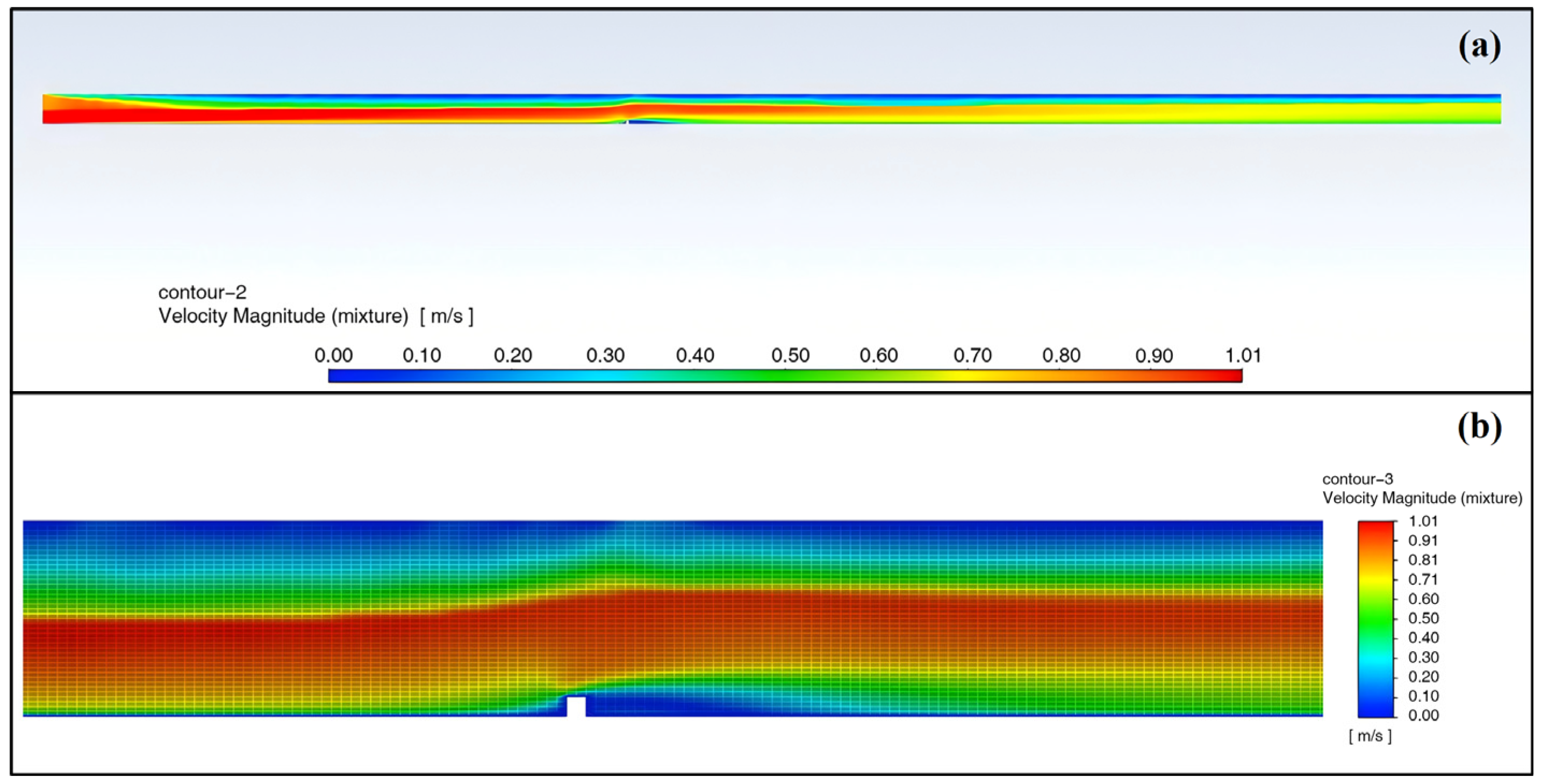
After the water flows past the baffle, the water surface is elevated. The distribution of velocity magnitudes in this flow field is illustrated in Figure 10.
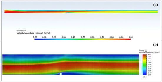
Figure 10.
(a) water–air flow velocity cloud image, (b) partial water–air flow velocity cloud image.
Figure 10 shows the distribution of water and air after the flow stabilizes. In the figure, red represents water and blue represents air. It is evident that the water flow decreases in velocity after passing around the baffle, resulting in an elevation of the water surface at the downstream end of the channel.
Figure 11 illustrates the local pressure distribution near the baffle, along with streamline and velocity vector diagrams.
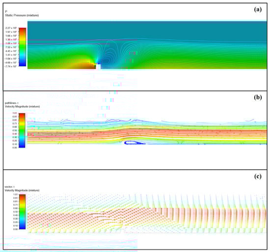
Figure 11.
Water–air flow: (a) pressure distribution cloud, (b) flow line, (c) velocity vector.
It can be observed that a reverse pressure gradient occurs near the baffle. Due to the fluid’s viscosity and the presence of the reverse pressure gradient, boundary layer separation undoubtedly occurs behind the baffle, leading to the formation of vortices. Water enters at a velocity of 1 m/s, and after flow stabilization, the boundary layer thickness is approximately 2 mm. Near the baffle, the boundary layer begins to thicken, reaching a maximum thickness of about 4.5 mm. After flowing past the baffle, the boundary layer thickness on the right side of the flow reaches around 3 mm.
Comparing the sedimentation positions of calcium carbonate particles in conditions 3.2 and 3.3, it is evident that the regions with higher calcium carbonate concentration coincide with areas where the boundary layer is thicker throughout the channel. This indicates that sedimentation of particles is more likely to occur in areas around the baffle and on the right side of the channel.
Figure 12 shows the structure of the particle sedimentation measurement section used in this simulation. The total length of the channel L(L1 + L2) is 400 mm, with a width W of 150 mm and a water flow height H of 10 mm. A piece of frosted glass is placed centrally in the channel, measuring 5 × 5 × 2 mm, positioned 100 mm from the inlet (distance L1). The direction of the water flow is along the positive x-axis. This model is employed to observe the motion trajectories of calcium carbonate micro-particles in the flow field. The total structured grid count is 535,400, and the minimum height of the mesh is 0.5 mm in the H1.
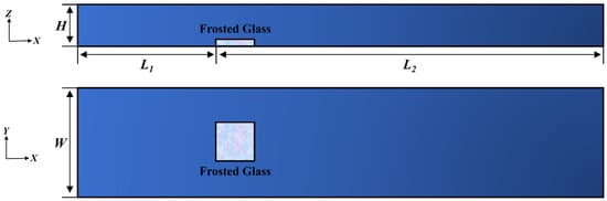
Figure 12.
Physical model of particle deposition measurement section.
Using the discrete phase model for calculations, the results are shown in Table 3. In this calculation, the calcium carbonate particles are considered rigid spheres with an average diameter of 3 × 10⁻⁶ m. The particle adhesion probability represents the ratio of the mass of particles that ultimately adhere to the bottom of the channel to the total mass of particles that collide with the bottom. The particle viscosity is used as the basis for determining the particle adhesion probability (η) [36].
Table 3.
Calculation results of CaCO3 particle deposition.
The adhesion probability can be calculated using the following relationship:
In the equation, μref represents the critical viscosity, and μp denotes the particle viscosity. In this simulation, μref is set to 100 mPa·S. The method for calculating the particle deposition rate is as follows:
Here, Nd and N0 represent the number of deposited particles, and the number of particles released at the pipe inlet, respectively.
From the CT cross-section of the sample, it can be seen that the size distribution of calcium carbonate (CaCO3) pores is uneven, with some pores being relatively large. The pore structure is modeled using a ball-and-stick approach, and the connected porosity, excluding dead pores, is 20.7%. The density of calcium carbonate is 2800 kg/m3, and the average particle diameter is 3 × 10⁻⁶ m. When the initial concentration is 0.01%, this corresponds to 9.982 × 10⁻2 kg/m3. In a water flow of 1 m/s, considering the saturation precipitation of the calcium carbonate solution, the total flow rate of calcium carbonate particles is 1.42 × 10⁻4 kg/s, resulting in a deposition rate of 0.371%. When the initial concentration is 0.001%, it corresponds to 9.982 × 10⁻3 kg/m3. In the same water flow of 1 m/s, the total flow rate of calcium carbonate particles is 7.05 × 10⁻6 kg/s, and the calculated deposition rate is also 0.371%. Based on these data estimates, the deposition velocities for calcium carbonate particles are 4.06 mm/a (0.001% CaCO3) to 81.7 mm/a (0.01% CaCO3). The observed deposition rate in the field is 4–6 mm/a, which is consistent with the simulation results.
The velocity and residence time of calcium carbonate particles in water are shown in Figure 13.
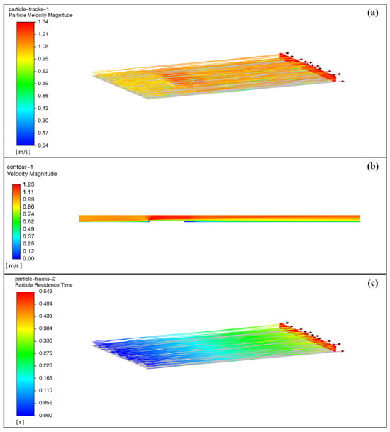
Figure 13.
Motion path of CaCO3 in water: (a) velocity, (b) cross-section velocity cloud image at W = 75 mm, (c) residence time.
In comparison, between Figure 13a,b it can be observed that the velocity of the particles is influenced by the velocity of the fluid at their location; that is, the faster the fluid velocity, the faster the particle velocity, and vice versa. As the particle velocity decreases, there is a higher likelihood of deposition occurring. The color adjustments represent the residence time of the particles, as shown in Figure 13c. If the particles do not experience deceleration, the time taken to pass through the channel is 0.40 s, while most of the particles leaving the channel have a residence time ranging between 0.38 and 0.43 s.
4. Conclusions
By sampling typical colorful pools in the Huanglong area and utilizing a Particle Image Velocimetry (PIV) system for the transient recording of flow field velocity distribution, as well as computational fluid dynamics (CFD) of ANSYS Fluent software to simulate the distribution, transport, and deposition processes of particles under different hydrodynamic conditions, the main conclusions are as follows:
1. In horizontal flow, the highest concentration of calcium carbonate reached 1.06%, an increase of 6% compared to the inlet. The accumulation occurred at the bottom right side of the flow, which is precisely where the flow boundary layer is thickest, indicating that calcium carbonate particles aggregated and settled within the flow boundary layer.
2. In the flow with an inclined surface and a baffle, the concentration of calcium carbonate significantly increased at the bottom right side of the channel and behind the baffle. This position corresponds to a slower flow velocity, where calcium carbonate particles are aggregated and settled in the low flow velocity region. Due to the presence of the boundary layer and low-speed vortex area, the particles experienced a decrease in velocity during transit, leading to calcium carbonate deposition as their flow velocity decreased. The areas with high concentrations of calcium carbonate particles coincided with regions of thicker boundary layers throughout the channel. Thus, the deposition of particles was more likely to occur before and after the baffle and on the right side of the channel.
3. Using the Discrete Phase Model (DPM), the motion trajectories of particles in the flow field were calculated. A total of 2424 particle trajectories were tracked, with 2415 particles leaving the computational channel and nine particles undergoing deposition. The deposition rate was 0.371%, with the deposition rate of calcium carbonate ranging from 4.06 mm/a to 81.7 mm/a, which is consistent with the observed data in the field.
Author Contributions
Methodology, X.L.; Writing – original draft, W.G.; Writing – review & editing, Y.Z. and W.Z.; Software, D.S.; Validation, S.W.; Formal analysis, J.D.; Investigation, H.C.; Supervision, Z.Z. and M.X.; Project administration, S.L. and H.X. All authors have read and agreed to the published version of the manuscript.
Funding
This work was financially supported by Sichuan Science and Technology Program (2024NSFSC0111), State Environmental Protection Key Laboratory of Synergetic Control and Joint Remediation for Soil & Water Pollution (GHBK-2023-01) and Sichuan Institute of Geological Survey (SDDY-Z2022008, SCIGS-CZDXM-2025010).
Data Availability Statement
The original contributions presented in this study are included in the article. Further inquiries can be directed to the corresponding authors.
Conflicts of Interest
The authors declare no conflict of interest.
References
- Pentecost, A. Travertine; Springer Science & Business Media: Berlin/Heidelberg, Germany, 2005. [Google Scholar]
- Khoury, H.N.; Clark, I.D. Mineralogy and origin of surficial uranium deposits hosted in travertine and calcrete from central Jordan. Appl. Geochem. 2014, 43, 49–65. [Google Scholar] [CrossRef]
- Wang, K.; Hu, S.; Li, W.; Liu, W.; Huang, Q.; Ma, K.; Shi, S. Depositional System of the Carboniferous Huanglong Formation, Eastern Sichuan Basin: Constraints from Sedimentology and Geochemistry. Acta Geol. Sin.-Engl. Ed. 2016, 90, 1795–1808. [Google Scholar] [CrossRef]
- Pentecost, A.; Viles, H. A review and reassessment of travertine classification. Géographie Phys. Quat. 1994, 48, 305–314. [Google Scholar] [CrossRef]
- Shi, Z.; Shi, Z.; Yin, G.; Liang, J. Travertine deposits, deep thermal metamorphism and tectonic activity in the Longmenshan tectonic region, southwestern China. Tectonophysics 2014, 633, 156–163. [Google Scholar] [CrossRef]
- Viles, H.; Pentecost, A. Tufa and travertine. In Geochemical Sediments and Landscapes; Wiley: Hoboken, NJ, USA, 2007; pp. 173–199. [Google Scholar]
- Luo, L.; Capezzuoli, E.; Vaselli, O.; Wen, H.; Lazzaroni, M.; Lu, Z.; Meloni, F.; Kele, S. Factors governing travertine deposition in fluvial systems: The Bagni San Filippo (central Italy) case study. Sediment. Geol. 2021, 426, 106023. [Google Scholar] [CrossRef]
- Croci, A.; Della Porta, G.; Capezzuoli, E. Depositional architecture of a mixed travertine-terrigenous system in a fault-controlled continental extensional basin (Messinian, Southern Tuscany, Central Italy). Sediment. Geol. 2016, 332, 13–39. [Google Scholar] [CrossRef]
- De Waele, J.; Gutiérrez, F. Karst Hydrogeology, Geomorphology and Caves; John Wiley & Sons.: Hoboken, NJ, USA, 2022. [Google Scholar]
- Zhang, T.; Dai, Q.; An, D.; Mors, R.A.; Li, Q.; Astini, R.A.; He, J.; Cui, J.; Jiang, R.; Dong, F.; et al. Effective mechanisms in the formation of pool-rimstone dams in continental carbonate systems: The case study of Huanglong, China. Sediment. Geol. 2023, 455, 106486. [Google Scholar] [CrossRef]
- Boussagol, P.; Vennin, E.; Monna, F.; Millet, L.; Bonnotte, A.; Motreuil, S.; Bundeleva, I.; Rius, D.; Visscher, P.T. Carbonate mud production in lakes is driven by degradation of microbial substances. Commun. Earth Environ. 2024, 5, 533. [Google Scholar] [CrossRef]
- Özkul, M.; Gökgöz, A.; Kele, S.; Baykara, M.O.; Shen, C.C.; Chang, Y.W.; Kaya, A.; Hançer, M.; Aratman, C.; Akin, T.; et al. Sedimentological and geochemical characteristics of a fluvial travertine: A case from the eastern Mediterranean region. Sedimentology 2014, 61, 291–318. [Google Scholar] [CrossRef]
- Ranade, V.V. Computational Flow Modeling for Chemical Reactor Engineering; Elsevier: Amsterdam, The Netherlands, 2001; Volume 5. [Google Scholar]
- Dianyu, E. Validation of CFD–DEM model for iron ore reduction at particle level and parametric study. Particuology 2020, 51, 163–172. [Google Scholar]
- Wu, W. Sediment Transport Dynamics; CRC Press: Boca Raton, FL, USA, 2023. [Google Scholar]
- Toker, E. Quaternary fluvial tufas of Sarıkavak area, southwestern Turkey: Facies and depositional systems. Quat. Int. 2017, 437, 37–50. [Google Scholar] [CrossRef]
- Iqbal, N.; Rauh, C. Coupling of discrete element model (DEM) with computational fluid mechanics (CFD): A validation study. Appl. Math. Comput. 2016, 277, 154–163. [Google Scholar] [CrossRef]
- Mahmoodi, B.; Hosseini, S.H.; Ahmadi, G. CFD–DEM simulation of a pseudo-two-dimensional spouted bed comprising coarse particles. Particuology 2019, 43, 171–180. [Google Scholar] [CrossRef]
- Marchelli, F.; Moliner, C.; Bosio, B.; Arato, E. A CFD-DEM sensitivity analysis: The case of a pseudo-2D spouted bed. Powder Technol. 2019, 353, 409–425. [Google Scholar] [CrossRef]
- Emam, S.A. Generalized Lagrange’s equations for systems with general constraints and distributed parameters. Multibody Syst. Dyn. 2020, 49, 95–117. [Google Scholar] [CrossRef]
- Paraskevopoulos, E.; Potosakis, N.; Natsiavas, S. An augmented Lagrangian formulation for the equations of motion of multibody systems subject to equality constraints. Procedia Eng. 2017, 199, 747–752. [Google Scholar] [CrossRef]
- Lin, S.; Cao, J.; Zhang, J.; Sun, T. Stability and convergence analysis for a new phase field crystal model with a nonlocal Lagrange multiplier. Math. Methods Appl. Sci. 2021, 44, 4972–4984. [Google Scholar] [CrossRef]
- Liu, Z.; Chen, S. Novel linear decoupled and unconditionally energy stable numerical methods for the modified phase field crystal model. Appl. Numer. Math. 2021, 163, 1–14. [Google Scholar] [CrossRef]
- Qian, Y.; Zhang, Y.; Huang, Y. Stability and error estimates of GPAV-based unconditionally energy-stable scheme for phase field crystal equation. Comput. Math. Appl. 2023, 151, 461–472. [Google Scholar] [CrossRef]
- Liu, Z.; Li, X. Efficient modified stabilized invariant energy quadratization approaches for phase-field crystal equation. Numer. Algorithms 2020, 85, 107–132. [Google Scholar] [CrossRef]
- Liang, Y.; Jia, H. Linear and unconditionally energy stable schemes for the modified phase field crystal equation. Comput. Math. Appl. 2024, 153, 197–212. [Google Scholar] [CrossRef]
- Seis, C. A Quantitative Theory for the Continuity Equation: Annales de l’Institut Henri Poincaré C, Analyse non linéaire; Elsevier: Amsterdam, The Netherlands, 2017. [Google Scholar]
- Brué, E.; Nguyen, Q.H. Sharp regularity estimates for solutions of the continuity equation drifted by Sobolev vector fields. Anal. PDE 2021, 14, 2539–2559. [Google Scholar] [CrossRef]
- Roth, G.A.; Aydogan, F. Derivation of new mass, momentum, and energy conservation equations for two-phase flows. Prog. Nucl. Energy 2015, 80, 90–101. [Google Scholar] [CrossRef]
- Jain, S.S.; Moin, P. A kinetic energy–and entropy-preserving scheme for compressible two-phase flows. J. Comput. Phys. 2022, 464, 111307. [Google Scholar] [CrossRef]
- Fuhrman, D.R.; Li, Y. Instability of the realizable k–ε turbulence model beneath surface waves. Phys. Fluids 2020, 32, 115108. [Google Scholar] [CrossRef]
- Larsen, B.E.; Fuhrman, D.R. On the over-production of turbulence beneath surface waves in Reynolds-averaged Navier–Stokes models. J. Fluid Mech. 2018, 853, 419–460. [Google Scholar] [CrossRef]
- Liu, Z.; Li, G. Numerical simulation of centrifugal pump impeller erosion caused by particles in lead–bismuth alloy. Int. J. Mod. Phys. B 2023, 37, 2350225. [Google Scholar] [CrossRef]
- Zhang, L.; Deng, C.; Liu, X. Energy transfer and interaction between liquid metal with water. Energy 2024, 288, 129865. [Google Scholar] [CrossRef]
- Saffman, P.G. The lift on a small sphere in a slow shear flow. J. Fluid Mech. 1965, 22, 385–400. [Google Scholar] [CrossRef]
- Reid, J.P.; Bertram, A.K.; Topping, D.O.; Laskin, A.; Martin, S.T.; Petters, M.D.; Pope, F.D.; Rovelli, G. The viscosity of atmospherically relevant organic particles. Nat. Commun. 2018, 9, 956. [Google Scholar] [CrossRef]


Disclaimer/Publisher’s Note: The statements, opinions and data contained in all publications are solely those of the individual author(s) and contributor(s) and not of MDPI and/or the editor(s). MDPI and/or the editor(s) disclaim responsibility for any injury to people or property resulting from any ideas, methods, instructions or products referred to in the content. |
© 2025 by the authors. Licensee MDPI, Basel, Switzerland. This article is an open access article distributed under the terms and conditions of the Creative Commons Attribution (CC BY) license (https://creativecommons.org/licenses/by/4.0/).