Prediction of Root-Zone Soil Moisture and Evapotranspiration in Cropland Using HYDRUS-1D Model with Different Soil Hydrodynamic Parameter Schemes

Abstract

This study provides a comprehensive assessment of the HYDRUS-1D model for predicting root-zone soil moisture (RZSM) and evapotranspiration (ET). It evaluates different soil hydrodynamic parameter (SHP) schemes—soil type-based, soil texture-based, and inverse solution—under varying cropping systems (Zea mays–Glycine max rotation and continuous Zea mays) and moisture conditions (irrigated and rainfed), aiming to understand water transport across different cultivation patterns. Using field measurements from 2002, the SHPs were optimized for each scheme and applied to predict RZSM and ET from 2003 to 2007. The inverse solution scheme produced nearly unbiased RZSM predictions with a root mean square error (RMSE) of 0.011 m³m⁻³, compared to RMSEs of 0.036 m³m⁻³ and 0.042 m³m⁻³ for the soil type-based and soil texture-based schemes, respectively. For ET predictions, comparable accuracy was achieved, with RMSEs of 66.4 Wm⁻², 69.5 Wm⁻², and 68.2 Wm⁻² across the three schemes. RZSM prediction accuracy declined over time in the continuous Zea mays field for all schemes, while systematic errors predominated in the Zea mays–Glycine max rotation field. ET accuracy trends mirrored RZSM in irrigated systems but diverged in rainfed croplands due to the decoupling of ET and RZSM under arid conditions.

1. Introduction

Global population growth and rising standards of living have increased pressure on food supply systems [1,2]. The global per capita cropland area decreased by approximately 10%, from 0.18 ha per person in 2003 to 0.16 ha per person in 2019 [3]. Additionally, this pressure has been further exacerbated because global national cereal (Zea mays, rice, and wheat) production during a drought was significantly reduced by 10.1% on average based on an extreme hydro-meteorological disaster survey between 1964 and 2007 [4]. Although extensive evidence of crop yield loss due to extreme temperatures or droughts has been reported, predicting heat and moisture stress in food systems adapting to climate change remains challenging [5,6,7,8,9]. As a result, food security continues to be a serious and widespread issue and is likely to increase, which requires the scientific management of water use in agriculture [10,11,12,13].

Agricultural drought typically follows meteorological drought, arising from sustained water deficits in croplands [14,15,16,17]. Soil moisture and evapotranspiration (ET) influence water and energy flows in the soil–vegetation–atmosphere system. These two variables are typically used to calculate water and heat balance and consequently provide scientific strategies for irrigation schemes [18,19,20,21,22,23,24,25]. Precipitation falls on croplands and infiltrates into the soil, reaching deeper layers. The root-zone soil moisture (RZSM) is then absorbed by plant roots for transpiration and growth, making RZSM more useful than surface soil moisture for agricultural applications. However, due to heterogeneous soil properties and limited detection techniques, obtaining spatially continuous datasets of RZSM and evapotranspiration (ET) over the crop growth period remains challenging [26,27,28]. Furthermore, due to complex physical and biological controls on water transport, various model estimates differ substantially. Specifically, the difference in average daily RZSM from eight global products exceeds 0.1 m³m⁻³, and total terrestrial ET derived among various models ranges from 50 to 80 km³ per year [29,30].

Currently, process-based models and machine-learning models are common and effective strategies for synchronously obtaining RZSM and ET with a consistent spatiotemporal scale. In particular, machine-learning methods, represented by deep learning models, have emerged since the 2000s, with a high correlation between predicted results and measured values [31,32,33]. However, the elevated expense of data acquisition and model training, as well as the black box of the process, limit the application of machine-learning methods to predict water transport. The process-based model differs from the machine-learning model in that it is based on the soil–plant–atmosphere continuum theory, which considers evaporation, root uptake, rainfall, groundwater, and runoff in the soil and their effects on the water content in the root zone [34,35]. Soil moisture simulations using process-based models typically require only a few precisely set key model parameters to predict RZSM and ET over a long time series and multi-depth soil profiles at a relatively low cost. Process-based soil moisture models have been developed based on different theories of soil moisture dynamics, mainly crops, land surface, and hydrological models [36,37,38]. To our knowledge, hydrological models give more consideration to the importance of soil hydrological properties for moisture movement, whereas crop and land surface models typically focus more on moisture-driven vegetation response problems and require additional vegetation parameter configurations. Although complex coupled models have been developed based on these three models, it also implies the need for more input parameters as increased uncertainty. Therefore, finding a balance between minimizing inputs, simplifying the process, and ensuring result comparability is crucial for accurately obtaining regional-scale RZSM and ET.

HYDRUS-1D is a one-dimensional hydrological model developed by the Salinity Laboratory of the United States Department of Agriculture, and the University of California, Riverside, to simulate water, solute, and heat transport in unsaturated media [39]. The HYDRUS-1D model can accurately simulate soil moisture with fewer soil and vegetation parameter configurations and has been widely used to study water recharge in agricultural systems [40,41,42,43,44]. Yu et al. (2022) [45] assessed the feasibility of using “low-cost” multi-source remote sensing data to optimize the parameters of the HYDRUS-1D model with five types of soil hydrodynamic parameter (SHP) acquisition methods. Yu et al. compared the results of different SHP methods for predicting RZSM in Zea mays fields. However, Feng et al. (2023) [46] reported that there are large differences in the modeling of water transport due to the partitioning of evaporation and transpiration, as well as drought conditions. This suggests that vegetation type and moisture conditions may be the main sources of uncertainty when applying HYDRUS-1D simulations to predict RZSM and ET. Although several studies have demonstrated the possibility of predicting RZSM and ET using the HYDRUS-1D model, respectively, a comprehensive assessment under different crop and moisture conditions is still lacking. Hydrological models are known to be very sensitive to hydrodynamic properties, but measuring SHPs in the field is difficult and costly. The use of pedotransfer functions (PTFs) and inverse methods are alternative approaches to obtain SHPs. The PTF is a soil database, which can derive SHPs from soil texture information. The inverse method is the least squares method based on historical data. It should be noted that SHPs derived from these two methods are not objective actual values, but rather equivalents based on statistical analysis. The fundamental principles of these two methods are distinct and may generate different SHPs for a given soil.

In general, these two methods have both merits and drawbacks. The use of SHPs derived from PTFs to predict RZSM and ET may lead to significant errors because the statistical functions created by the soil database cannot fully account for all variability in these processes. On the other hand, the inverse method is difficult to generalize to regional scales because it requires calibration of field data that are never acquired on a regional scale. In this study, three sites containing irrigated and rainfed Zea mays, and Zea mays–Glycine max rotation croplands from the AmeriFlux network, were selected to assess the accuracy of the RZSM and ET predictions during the crop growth period. The hydrodynamic properties and meteorological factors are similar there, yet the crops and water conditions exhibit notable differences. The objectives of this study are (1) to quantify uncertainties in RZSM and ET predictions arising from SHP estimation methods; (2) to investigate how variability in crop type and moisture regimes (irrigated vs. rainfed) influences model accuracy; (3) to identify key factors limiting the spatiotemporal scalability of the HYDRUS-1D model for regional hydrologic applications. By comparing the results of predicting RZSM and ET using different SHP methods for a given soil, the variability of different methods will be investigated under various crops and moisture conditions. Specifically, SHPs are obtained using historical data from 2002 and then applied to the predictions of RZSM and ET from 2003 to 2007. Finally, the results of predicting RZSM and ET using different SHP schemes are evaluated to clarify the main factors affecting the spatiotemporal expansion of the HYDRUS-1D model.

2. Materials and Methods

2.1. Site Description

We selected three croplands (US-Ne1, US-Ne2, and US-Ne3) from the Central Plains of the United States that provide sufficient uniform crop cover to adequately measure soil moisture and energy fluxes using tower eddy covariance systems [47,48,49]. The three sites are located at the University of Nebraska Agricultural Research and Development Center, near Mead, NE, USA. As shown in Figure 1, the US-Ne1 and US-Ne2 fields are circular with a radius of ~390 m, and both are equipped with center-pivot irrigation systems. The US-Ne3 site is a 790-m-long square field that relies entirely on rainfall. The first field (US-Ne1) is a field that has been planted with Zea mays for years, while the other two fields (US-Ne2 and US-Ne3) are Zea mays–Glycine max rotation fields. The climate type of the farm belongs to Dfa based on the Köppen–Geiger climate classification, with ~362 m average elevation, ~10 °C mean annual temperature, and ~790 mm mean annual precipitation. Soil samples are collected from the 180 cm soil column. Analysis of the samples reveals that the soil is deep silty clay loams, consisting of four soil series at all three sites: Yutan (fine-silty, mixed, superactive, mesic Mollic Hapludalfs), Tomek (fine, smectitic, mesic Pachic Argialbolls), Filbert (fine, smectitic, mesic Vertic Argialbolls), and Filmore (fine, smectitic, mesic Vertic Argialbolls). Details of soil texture are provided in

Table 1. Latitude, longitude, soil texture, and planting at the cropland sites.

Site	Latitude	Longitude	Clay	Sand	Planting
US-Ne1	41.1651	−96.4766	37	11	Zea mays
US-Ne2	41.1649	−96.4701	33	12	Zea mays, Glycine max
US-Ne3	41.1797	−96.4397	35	8	Zea mays, Glycine max

. In addition, no tilling has been practiced at any site since its inception in 2001. In this system, seeds are planted directly underneath the stubble of the existing crop in previous years, with no soil disturbance other than the planter opening a narrow slot for seed placement.

Soil moisture data were collected at four depths (0.10, 0.25, 0.50, and 1.0 m) at each site, with three spatially distributed observations per depth. The observation time-step was hourly. In the present study, the measured RZSM was computed as a depth-weighted mean of the values in the range of 0–100 cm [50], which represents most of the temporal dynamics of the soil moisture that is available for root water uptake of crop. In addition, automatic weather stations, eddy covariance systems, and four-component radiometers were installed at each site to acquire meteorological, radiation, and ET data. The irrigation volumes of US-Ne1 and US-Ne2 were not directly accessible and needed to be calculated from the precipitation through comparison with US-Ne3. Specifically, the three sites were situated nearby (less than 1.6 km apart) and the meteorological conditions were deemed to be comparable. In the absence of precipitation at US-Ne3 (rainfed field), the precipitation observed at US-Ne1 and US-Ne2 (irrigated field) was regarded as irrigation. The leaf area index (LAI) and plant height were estimated from destructive sampling at 10–14 day intervals until physiological maturity and before harvest. Samples were taken from 1 m linear row sections at approximately six different locations at each site. US-Ne2 and US-Ne3 are Zea mays–Glycine max rotation sites, where Glycine max was planted in 2002, 2004, and 2006, and Zea mays was planted in 2003, 2005, and 2007. Several outliers for plant height and the LAI were flagged and then rejected when calibration was implemented, for example, plant height measurements on 28 July 2006, and LAI measurements on 19 September 2005. The dataset is publicly available ground-based observation data, which can be freely downloaded from the website https://fluxnet.org (accessed on 26 February 2025). The main data inputs include soil properties (soil texture percentages, soil heat flux and soil moisture), vegetation parameters (vegetation height and leaf area index) and atmosphere factors (radiation, air temperature, and air humidity).

2.2. HYDRUS-1D Model

The HYDRUS-1D model (version 4.17), developed by the USDA Salinity Laboratory and the University of California, Riverside, simulates water, heat, and solute movement in variably unsaturated media under different soil, vegetation, and climatic conditions [39]. In HYDRUS-1D, the equations are solved by spatial discretization of the soil profile using the Galerkin finite element method in an implicit difference format, which is suitable for simulating soil moisture in the root domain. Since 1994, studies have demonstrated relatively satisfactory results from this model for surface energy balance, soil CO₂ fluxes, soil moisture, and solute transport [35,39,40,41,42,45]. The HYDRUS-1D model could capture real-time changes in the ET and RZSM with high accuracy and robustness. In the present study, the HYDRUS-1D model was used to predict ET and RZSM in irrigated and rainfed croplands during the growth period. In this model, the water transport in a variably saturated medium follows Richard’s equation, which was first proposed by Richards (1931) [51] to describe the flow of fluids in unsaturated porous mediums:

$${\displaystyle \frac{\partial \theta (\psi )}{\partial (t)}}={\displaystyle \frac{\partial }{\partial z}}\left[K(\psi )({\displaystyle \frac{\partial \psi }{\partial z}}+1)\right]-S_v(\psi )$$

(1)

where ψ is the water pressure head (cm), θ(ψ) is the volumetric water content at a point in the soil profile (cm³cm⁻³), t is time (h), z is the spatial coordinate (cm) (positive upward), K(ψ) is the hydraulic conductivity (cm h⁻¹), and S_v(ψ) is the sink term that accounts for root water uptake (cm³cm⁻³h⁻¹).

HYDRUS-1D allows the selection of six types of models for soil hydraulic properties. In the present study, the van Genuchten–Mualem (1980) [52] model was used to describe the retention curve of the soil moisture profile and estimate the saturated hydraulic conductivity. The model has been shown to describe well the vast majority of soil hydraulic property characteristics in nature as follows:

$$\theta (\psi )=\left\{\begin{array}{cc}{\theta }_r+{\displaystyle \frac{{\theta }_s-{\theta }_r}{{\left[1+{\left|\alpha \psi \right|}^n\right]}^m}}& \psi <0\\ {\theta }_s& \psi >0\end{array}\right.$$

(2)

$$K(\psi )=K_s{S}_e^l{[1-{(1-S_e^{l/m})}^m]}^2$$

(3)

where θ_r and θ_s are the residual and saturated water content, respectively, (cm³cm⁻³); α (>0, in cm⁻¹) is related to the inverse of the air entry suction, n (>1) describes the pore size distribution, m = 1 − 1/n, K_s is the saturated hydraulic conductivity (cm/days), l is the pore tortuosity/connectivity index, and S_e is the relative saturation. Therefore, the spatial heterogeneity of soil hydraulic properties for the van Genuchten–Mualem model is characterized by six main SHPs, including θ_r, θ_s, α, n, K_s, l, which requires the calibration of these SHPs under different soil conditions.

Actual ET is divided into two independent processes in HYDRUS-1D, which consist of evaporation from soil surface, and transpiration from vegetation. Actual evaporation was derived by the Richards equation, with the soil–atmosphere boundary condition, which can be obtained by limiting the absolute value of the surface flux as following two conditions:

$$\left|-K{\displaystyle \frac{\partial h}{\partial x}}-K\right|\le E_p$$

(4)

$$h_A\le h\le h_S$$

(5)

where E_p is the potential infiltration or evaporation for the given atmospheric conditions, K is unsaturated soil hydraulic conductivity, h is pressure head, x is soil boundary length, and h_A and h_S are minimum and maximum h at the soil surface allowed under the prevailing soil conditions. The value for h_A is determined by soil moisture and water vapor at the boundary, whereas h_S is usually set to zero. When one of the conditions is satisfied, a prescribed head boundary condition (h) will be used to estimate the actual evaporation by the Richards equation. If h exceeds h_A, it indicates that there is sufficient water in the soil profile to meet atmospheric demand, at which point actual evaporation equals potential evaporation. When h is less than h_A, the actual evaporation is zero.

The h_A represents the minimum allowable surface pressure head for the prevailing soil conditions, derived from the equilibrium between water vapor and soil moisture in the atmosphere. It can be calculated by the following formula:

$$h_A=-{\displaystyle \frac{RT}{Mg}}In(H_r)$$

(6)

where R is the gas constant (8.314 Jmol⁻¹K⁻¹), T is air temperature (K), M is the molecular weight of water (0.018015 kgmol⁻¹), g is the gravitational acceleration (9.81 ms⁻²), and H_r is air humidity.

The groundwater table in the three fields was deep without local groundwater recharge and the plot perimeter was in a free drainage state. Therefore, the lower boundary condition of the HYDRUS-1D model is free drainage. The depth of the soil profile was set to 120 cm. The number of soil materials is one.

Actual transpiration and RZSM are linked via the root water uptake model in HYDRUS-1D, which is defined as the volume of water removed from a unit volume of soil per unit of time due to plant water uptake as follows:

$$S(h)=\alpha (h)b(x)T_p$$

(7)

where S(h) is the volume of water uptake from vegetation, α(h) is the root-water uptake water stress response function which is a prescribed dimensionless function of the soil moisture pressure head (0 ≤ α ≤ 1), and b(x) is the normalized water uptake distribution function, which describes the spatial variation of the potential extraction term over the root zone, and T_p is potential transpiration.

The Feddes model was used to describe the relationship between root water uptake and pressure head, namely, α(h). The b(x) is an exponential function which assumes that the effective water-absorbing roots are proportional to the distribution of root density in the soil profile and pressure head. The T_p can be calculated from potential ET (ET₀) using Beer’s law that partitions the solar radiation component of the energy budget via interception by the canopy as:

$$T_p=E{T}_0(1-e^{-k\ast LAI})$$

(8)

where k is an extinction coefficient, which mainly depends on the canopy distribution. It can be set as 0.5–0.75. Further details on the methodology can be found in [45].

Moreover, ET₀ was calculated using the Penman–Monteith equation (1965) [53], which divides ET into two parts depending on the driving element: the radiation term ET_rad and the aerodynamic term ET_aero:

$$E{T}_0=E{T}_{rad}+E{T}_{aero}={\displaystyle \frac{1}{\lambda }}\left[{\displaystyle \frac{\Delta (R_n-G)}{\Delta +\gamma (1+r_c/r_a)}}+{\displaystyle \frac{\rho c_p(e_s-e_a)/r_a}{\Delta +\gamma (1+r_c/r_a)}}\right]$$

(9)

where R_n and G are the net radiation and soil heat fluxes at the surface, respectively, r_c is the surface resistance which can be estimated by 100/LAI, r_a is the aerodynamic resistance, e_s and e_a are the saturated and actual water vapor pressure, respectively, c_p is the constant pressure of specific heat of air, and γ is the wet and dry table constant. ET₀ is the evaporation from an extended surface of a short crop which fully shades the ground with the negligible resistance to the water flow in the soil–vegetation–atmosphere continuum. Actual ET is usually estimated by multiplying the reference ET by the crop coefficient and the soil moisture stress coefficient. Further details can be found in Allen et al. (1998) [54].

Interception (I) can be considered when the LAI is entered. The I is defined as follows:

$$I=a\cdot LAI(1-{\displaystyle \frac{1}{1+\frac{bP}{a\cdot LAI}}})$$

(10)

where a and b are empirical constants (for ordinary agricultural crops a ≈ 0.025 cmday⁻¹, b ≈ 1 − e^−kLAI).

The I represents evaporation from wet leaf, including irrigation and precipitation. ET can be calculated as the total of evaporation from soil surface and wet leaf, and transpiration from vegetation. Here, transpiration is derived by calculating the amount of water absorbed.

2.3. Soil Hydraulic and Vegetation Parameters

Determination of the SHPs in Equations (2) and (3) are prerequisites for applying hydrological models to predict RZSM and ET with satisfactory accuracy because they determine the amount of energy required to transport soil moisture. However, measuring SHPs in bulk at the field scale is difficult and time-consuming. In previous studies, three methods have been commonly used to obtain SHP: (1) obtaining the SHP from Carsel and Parrish (1988) [55] under different soil texture conditions (Model I); (2) estimating the SHP through PTFs in a hierarchical manner from soil textural class information, including the proportion of soil components (sand, silt, and clay) and bulk density (Model II); and (3) estimating the SHP through the least-squares method on the inverse solution of historical soil moisture and meteorological data (Model III). Theoretically, SHPs from Model I and Model II are obtained using PTFs from soil databases, while Model III is an inverse solution based on historical soil moisture and meteorological data by a mathematical method. It is noted that Model I and Model II require soil information as input, whereas Model III does not. Moreover, when using the Model I and II schemes, all SHPs can be obtained except for the l-parameter in the hydraulic conductivity function, which represents the effects of tortuosity and pore connectivity. Introducing the l-parameter into the hydraulic conductivity function is useful for increasing the degrees of freedom during the optimization of well-defined experimental data, such as the multistep outflow and evaporation methods. The l-parameter value was initially estimated to be 0.5 by Mualem (1976) [56], but Schaap and Leij (2000) [57] suggested that the l-parameter should have a value of −1 after analyzing the Unsaturated Soil Hydraulic Database. Although these findings provide a far better description of unsaturated hydraulic conductivity data, it also indicates that the l-parameter is usually empirical. Better results are commonly obtained using Model III because it can optimize more parameters than Models I and II. Therefore, Method III was first used to predict RZSM and ET. Methods I and II are shown in the discussion as controls.

A few vegetation parameters, including vegetation height, LAI, and root depth, are required as inputs to predict RZSM and ET. The three cropland sites provided samples for measuring plant height and LAI at 10–14 day intervals. However, this was not sufficient to characterize the state of vegetation during the rapid growth period. Therefore, a fit–fill scheme was implemented to generate continuously varying vegetation parameters [58,59]. Specifically, the continuous plant height can be expressed as:

$$H=a/(1+b\times \exp (-c\times x))$$

(11)

where a, b, and c are the fitting coefficients, x is the discrete observation of the plant height, and H denotes the continuous plant height over time. The logarithmic function and its modified versions have been shown to be successful at fitting plant height curves.

The least-squares regression method is one of the most widely used statistical filtering methods for reconstructing time series data and is suitable for environments where the change in the LAI follows regular vegetation cycles of growth and decline [60]. In the present study, a temporal least-squares inversion method was adopted to estimate the LAI during the crop growth period based on previous studies [61,62]. In the study, a least-squares method of curves was employed to reconstruct LAI growth curves, which require the optimal regression function by minimizing the following cost (error) function:

$$error=p\underset{error measure}{\underbrace{{{\displaystyle \sum _i{w}_i(y_i-s(x_i))}}^2}}+(1-p)\underset{roughness measure}{\underbrace{{\displaystyle \int {(\frac{d^{2}s}{d{x}^2})}^{2}dx}}}$$

(12)

where w_i is the specified weight, p is the smoothing parameter defined between 0 and 1, and y_i and s(x_i) are the discrete LAI measurements and the reconstructed temporal continuous LAI, respectively.

Root depth data was not provided for the three sites. The study showed that LAI explained 80–89% of the variation in root depth [63]. For annual vegetation types, changes in root depth typically follow the LAI, which indicates LAI growth rates are approximately linearly correlated with root depth. The maximum root depth applies to the maximum LAI period, whereas temporal changes in root depth are assumed to be constant after LAI is maximum [64]. Hence, the root depth of a crop is directly linked to the dynamics of the derived LAI:

$$R{D}_i=R{D}_{max}{\displaystyle \frac{LA{I}_i-LA{I}_{min}}{LA{I}_{max}-LA{I}_{min}}}$$

(13)

where RD_i is the continuous plant height over time, RD_max is the maximum root depth of the vegetation, LAI_i is the continuous LAI over time, and LAI_min and LAI_max are the minimum and maximum LAIs of the vegetation over time, respectively. In the present study, RD_max was set to 120 cm.

In the present study, the three metrics of the coefficient of determination (R²), bias and root mean square error (RMSE) were used to evaluate the performance of the HYDRUS-1D model in predicting RZSM and ET and vegetation biometric reconstruction. The three metrics can be written as follows:

$${\mathrm{R}}^2=1-{\displaystyle \frac{{\displaystyle \sum \begin{array}{c}n\\ i=1\end{array}}{(y_i-{\widehat{y}}_i)}^2}{{\displaystyle \sum \begin{array}{c}n\\ i=1\end{array}}{(y_i-{\overline{y}}_i)}^2}}$$

(14)

$$\mathrm{bias}={\displaystyle \frac{1}{N}}{\displaystyle \sum \begin{array}{c}n\\ i=1\end{array}}({\widehat{y}}_i-y_i)$$

(15)

$$\mathrm{RMSE}=\sqrt{{\displaystyle \frac{1}{N}}{\displaystyle \sum \begin{array}{c}n\\ i=1\end{array}}{({\widehat{y}}_i-y_i)}^2}$$

(16)

where y_i is the measured value from AmriFlux, $\overline{y}$_i is the average value of y_i, N is the total number, $\widehat{y}$_i is the predicted value.

3. Results

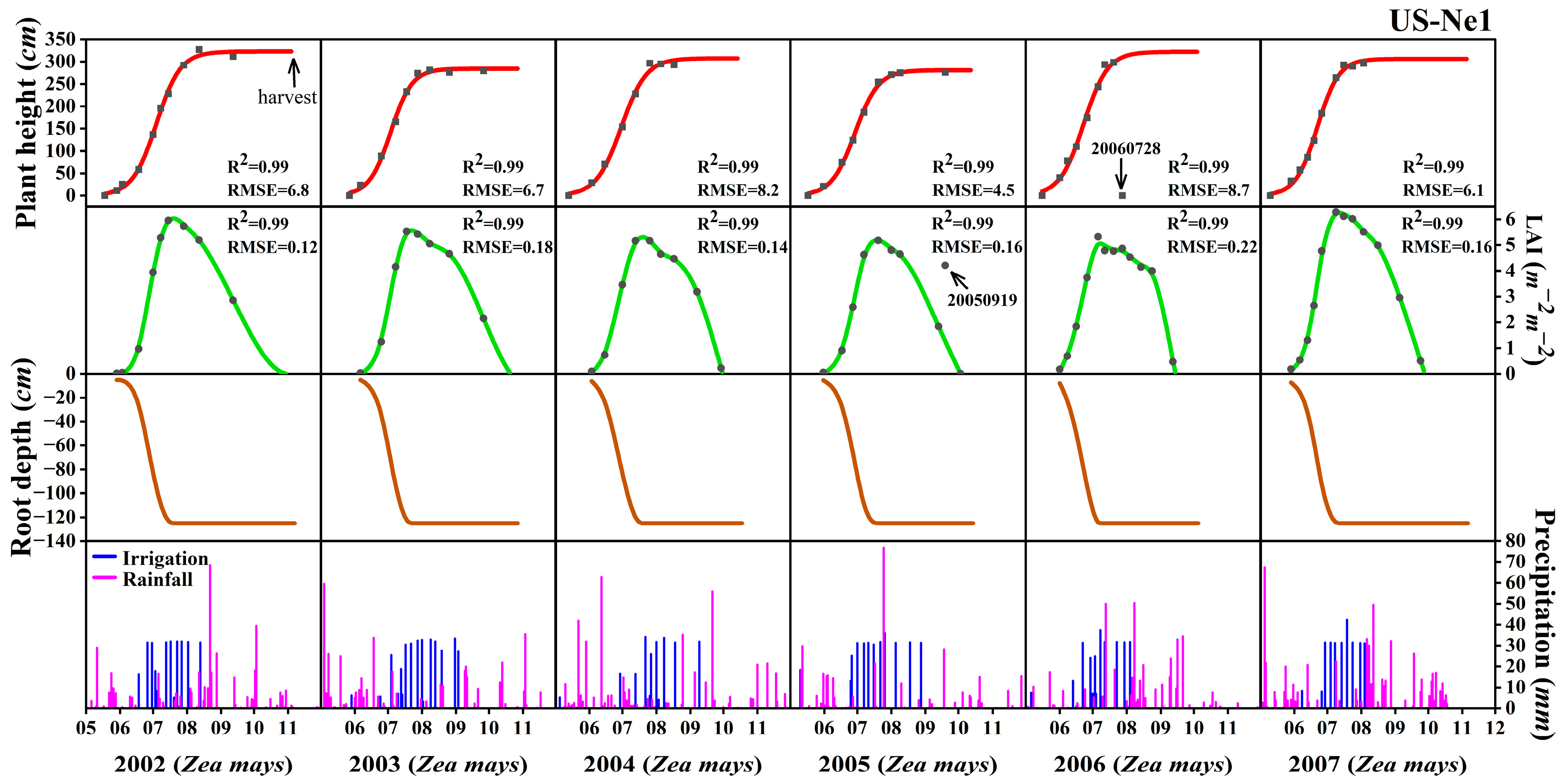
3.1. Determination of Soil and Vegetation Parameters

In the present study, SHPs firstly are obtained by Model III because of uncertainties of the l-parameter. Subsequently, SHPs obtained in 2002 at the three sites were applied to predict the RZSM and ET during the crop growth period (sowing to harvesting) from 2003 to 2007. The results of RZSM fitting in 2002 based on Model III are shown in Figure 2 for US-Ne1, US-Ne2, and US-Ne3, with R² values of 0.91, 0.85, and 0.90, MAE of 0.004 m³m⁻³, 0.005 m³m⁻³, and 0.010 m³m⁻³, and root mean square error (RMSE) of 0.005 m³m⁻³, 0.007 m³m⁻³, and 0.012 m³m⁻³, respectively. The inverse solution obtained almost unbiased results for RZSM, while the RZSM of US-Ne3 was slightly overestimated. It is understandable that the RZSM in irrigated areas would typically remain high during crop growth periods, whereas rainfed fields would have a more variable RZSM due to droughts. Soil characteristic curves can reflect the relationship between soil moisture energy and quantity, which means that considerable ET results can also be obtained based on the water and energy balance. Comparing the Model I and II schemes, all six parameters can be obtained simultaneously using Model III. The SHPs using Model III are listed in

Table 2. SHPs derived from inverse solution method in 2002.

Site	θr	θs	α (1/cm)	n	Ks (cm/Hours)	l
US-Ne1	0.2	0.47	0.0007	1.36	0.16	2.36
US-Ne2	0.19	0.47	0.002	1.15	0.29	1.15
US-Ne3	0.14	0.49	0.0013	1.51	2.1	6.98

. It should be noted that the SHPs from Model III are not covariates in the physical sense, but equivalent covariates within 120 cm soil depth estimated based on mathematical iterative methods, which are common and effective practices for moisture simulation. As a result, the SHPs of the soil with similar soil texture percentages may be different when Model III is used.

The calibrated vegetation parameters, including plant height, LAI, root depth, and irrigation amount, at the US-Ne1, US-Ne2, and US-Ne3 sites are shown in Figure 3, Figure 4 and Figure 5, respectively, where the black dots are the measured values. These results show good calibration results for vegetation parameters at the US-Ne1 site from 2002 to 2007, with an average R² of 0.99 and an average RMSE of 6.8 cm for plant height, and an average R² of 0.99 and average RMSE of 0.16 m²/m² for LAI. The annual maximum plant height of Zea mays is 276.2–312.6 cm, and the annual maximum LAI is 5.16–6.28 m²/m². The root depth increased curvilinearly before the LAI reached its maximum value and remained constant after LAI reached its maximum value. Moreover, irrigation mainly occurred during rapid crop growth from July to September, and the maximum daily irrigation was ~30 mm.

The calibrated vegetation parameters and irrigation amounts in US-Ne2 are shown in Figure 4. Regarding Glycine max, a reasonable calibration result was found with a 3 year average RMSE of 4.5 cm for plant height and 0.29 m²/m² for the LAI. The average RMSE of plant height and the LAI for Zea mays were 6.4 cm and 0.27 m²/m², respectively. In summary, Zea mays plant height calibration exhibited marginally lower accuracy compared to Glycine max, while LAI calibration demonstrated comparable performance between the two crops. Furthermore, the annual plant height of Glycine max was ~100.0 cm, and the annual maximum LAI was 4.40–5.78 m²/m². Notably, the LAI of Glycine max typically reached its maximum later than that of Zea mays, indicating that the root depth of Glycine max reached its maximum later than that of Zea mays.

As a control for US-Ne2, US-Ne3 was a rainfed, Zea mays–Glycine max rotation site with calibrated vegetation parameters, as shown in Figure 5. Calibration results in the US-Ne3 site for Glycine max showed an average RMSE of 3.9 cm for plant height and 0.24 m²/m² for LAI. The average RMSE of plant height and the LAI for Zea mays were 3.0 cm and 0.16 m²/m², respectively. The maximum LAI and plant height in rainfed fields were usually smaller than those in irrigated fields because rainfed crops were subjected to water stress during growth. As for the Glycine max, the maximum plant heights in 2002, 2004, and 2006 were 76.5 cm, 85.7 cm, and 98.5 cm, respectively, and the maximum LAI in 2002, 2004, and 2006 were 3.03 m²/m², 4.41 m²/m², and 4.48 m²/m², respectively. In rainfed fields, crop growth depends on precipitation. A large amount of precipitation occurred between July and September 2006 compared with that in 2002 and 2004. For Zea mays, the maximum plant height in 2003, 2005, and 2007 was 243.1 cm, 252.9 cm, and 251.4 cm, respectively, and the maximum LAI in 2003, 2005, and 2007 was 4.27 m²/m², 4.33 m²/m², and 4.12 m²/m², respectively. The smallest maximum plant height was found in 2003 because the precipitation in 2003 was significantly less than that in 2005 and 2007. Although the maximum LAI was comparable among the 3 years, it declined rapidly in 2003 after peaking because of water stress.

In this section, vegetation growth curves (plant height and LAI) were reconstructed using discrete measurement data (black point in Figure 3, Figure 4 and Figure 5). Overall, there was good agreement (R² = 0.99) between the vegetation growth curves and the measurement data. On the other hand, vegetation growth curves also differed under various crop and moisture conditions. Comparison of irrigated and rainfed cropland dominated the importance of soil moisture for proper vegetation growth, thus highlighting the significance of predicting RZSM and ET.

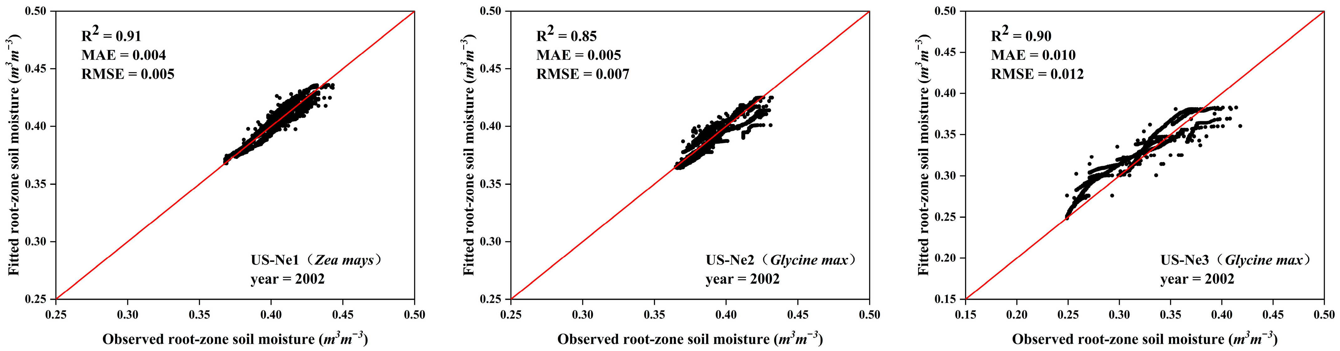
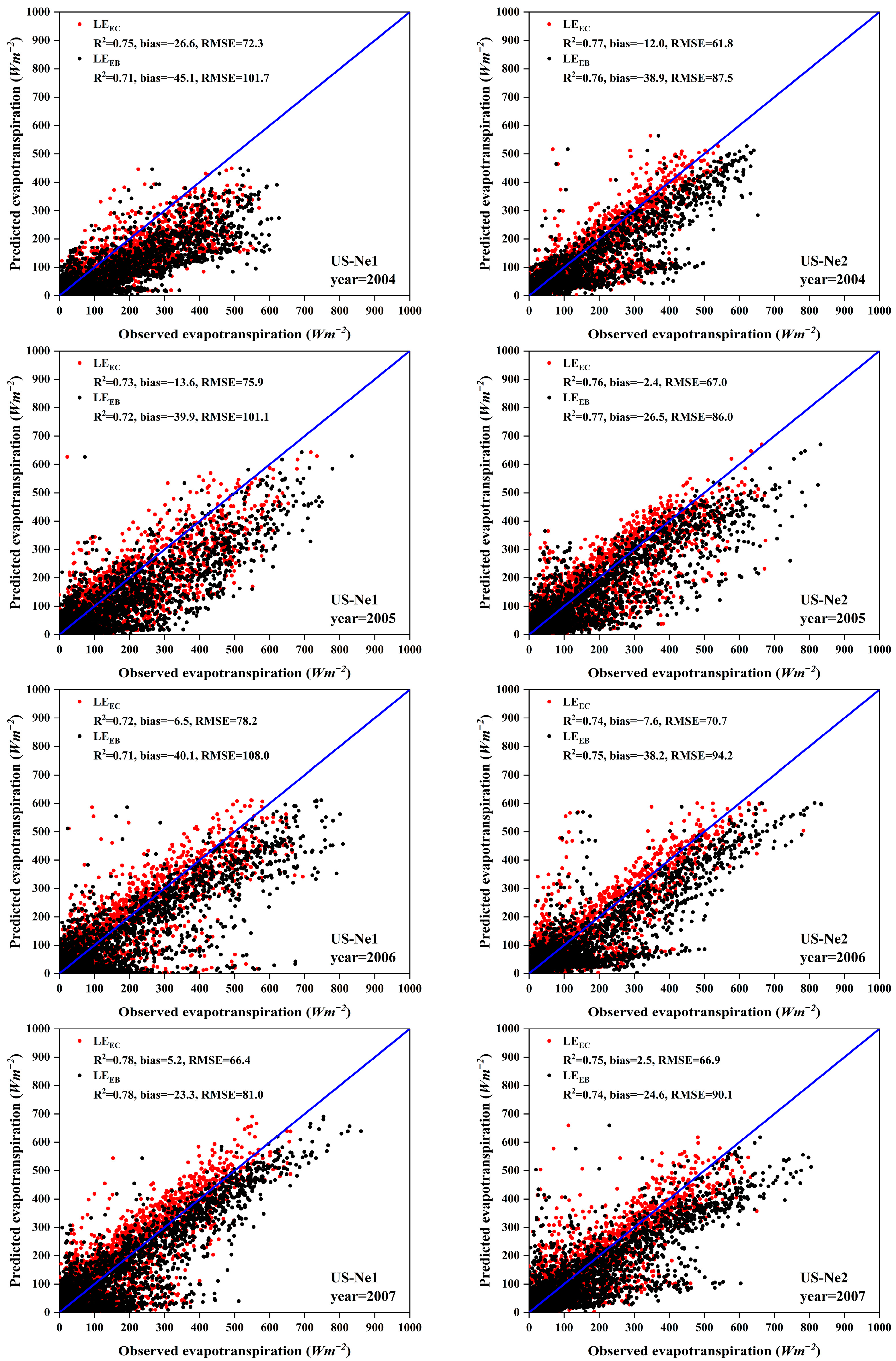
3.2. RZSM and ET Prediction in Irrigated Cropland

Results of the RZSM prediction using the HYDRUS-1D model in irrigated croplands (US-Ne1 and US-Ne2) during the crop growth period (sowing to harvesting) from 2003 to 2007 are shown in Figure 6. The R² of the two sites between predicted and measured RZSM ranged from 0.56 to 0.88, with an average R² of 0.75; bias ranged from −0.004 to 0.008 m³m⁻³; and RMSE ranged from 0.005 to 0.012 m³m⁻³, with an average RMSE of 0.009 m³m⁻³. In summary, an almost unbiased result was obtained for predicting RZSM in irrigated croplands.

As for the irrigated continuous-Zea mays field (US-Ne1), the soil in the root zone was usually kept wet during crop growth, and the RZSM was 0.33–0.47 m³m⁻³. The R² values of the RZSM between predictions and observations from 2003 to 2007 were 0.88, 0.75, 0.85, 0.66, and 0.82, respectively. Meanwhile, the bias was 0.003 m³m⁻³, −0.004 m³m⁻³, 0.008 m³m⁻³, 0.003 m³m⁻³, and 0.003 m³m^−3, and the RMSE was 0.007 m³m⁻³, 0.008 m³m⁻³, 0.012 m³m⁻³, 0.011 m³m⁻³, and 0.008 m³m⁻³, respectively. The predicted RZSM was overestimated during the early stages of crop growth in 2005. In addition, changes in RZSM were not well-captured after precipitation or irrigation in 2006 because RZSM was not steady at this time. In the irrigated Zea mays–Glycine max rotation field (US-Ne2), comparable precision was found between the predicted and observed RZSM from 2003 to 2007, with R² values of 0.73, 0.81, 0.73, 0.75, and 0.56; biases of 0.003 m³m⁻³, −0.002 m³m⁻³, −0.004 m³m⁻³, −0.003 m³m⁻³, and −0.003 m³m⁻³; and RMSE of 0.010 m³m⁻³, 0.005 m³m⁻³, 0.010 m³m⁻³, 0.007 m³m⁻³, and 0.007 m³m⁻³, respectively.

Scatter plots of the predicted and measured ET in the irrigated croplands are shown in Figure 7. The ET predicted using HYDRUS-1D is the amount of water consumed through evaporation and transpiration, whereas the sites typically measure latent heat (LE). Therefore, in our study, the predicted ET values were converted into energy units to match the measurements. In addition, to fully evaluate the predicted ET, the LE was derived through eddy covariance-based (LE_EC) and energy balance-based (LE_EB = R_n–H–G) methods were compared with the predicted ET. Overall, reasonable accuracy was obtained for irrigated croplands in the predicted ET compared with the observations. The R² of the two sites (US-Ne1 and US-Ne2) between the predicted ET and LE_EC was in the range of 0.72 to 0.80, with an average R² of 0.76; bias ranged from −26.6 to 25.2 Wm⁻²; and RMSE ranged from 61.8 to 78.2 Wm⁻², with an average RMSE of 70.3 Wm⁻². However, an overall underestimation was found between predicted ET and LE_EB in croplands from 2003 to 2007, with R² of 0.71–0.79 (average, 0.75), with bias of −45.1 to −0.10 Wm⁻², and RMSE of 77.3–108.0 Wm⁻² (average, 90.9 Wm⁻²). It should be noted that the LE derived from energy balance-based observations can be high relative to that derived from eddy covariance-based observations because the energy balance equation assigns the uncertain energy portion of the observation to the LE term.

For the US-Ne1 site, comparable accuracy was obtained over time. The R² between the predicted ET and LE_EC ranged from 0.72 to 0.79, and that between the predicted ET and LE_EB ranged from 0.71 to 0.79. The bias of predicted ET and LE_EC was −26.6 to 12.8 Wm⁻², and that of predicted ET and LE_EB was −45.1 to −6.10 Wm⁻², respectively. The RMSEs between the predicted ET and LE_EC from 2003 to 2007 were 67.7 Wm⁻², 72.3 Wm⁻², 75.9 Wm⁻², 78.2 Wm⁻², and 66.4 Wm⁻², respectively, and those between the predicted ET and LE_EB were 77.3 Wm⁻², 101.7 Wm⁻², 101.1 Wm⁻², 108.0 Wm⁻², and 81.0 Wm⁻², respectively. The overall underestimation between the predicted ET and LE_EB resulted in a loss of accuracy from 2004 to 2006. For the US-Ne2 site, the R² between the predicted ET and LE_EC was from 0.74 to 0.80, and that between the predicted ET and LE_EB was from 0.74 to 0.78. The bias of predicted ET and LE_EC was −12.0 to 25.2 Wm⁻², and that of the predicted ET and LE_EB was −38.9 to −0.10 Wm⁻², respectively. The RMSE between the predicted ET and LE_EC from 2003 to 2007 was 76.0 Wm⁻², 61.8 Wm⁻², 67.0 Wm⁻², 70.7 Wm⁻², and 66.9 Wm⁻², respectively, and that between the predicted ET and LE_EB was 81.7 Wm⁻², 87.5 Wm⁻², 86.0 Wm⁻², 94.2 Wm⁻², and 90.1 Wm⁻², respectively.

3.3. RZSM and ET Prediction in Rainfed Cropland

The rainfed site (US-Ne3) was different from the US-Ne1 and US-Ne2 sites. Scatter plots of the predicted and measured RZSM, and the predicted and measured ET at the US-Ne3 site from 2003 to 2007, are shown in Figure 8. The R² of RZSM between predictions and observations from 2003 to 2007 was 0.87, 0.97, 0.97, 0.83, and 0.84, respectively. The bias was −0.005 m³m⁻³, −0.015 m³m⁻³, 0.005 m³m⁻³, −0.004 m³m⁻³, and −0.005 m³m⁻³, respectively, and the RMSE was 0.014 m³m⁻³, 0.021 m³m⁻³, 0.012 m³m⁻³, 0.021 m³m⁻³, and 0.013 m³m⁻³, respectively. The multi-year average R², bias, and RMSE were 0.90, −0.005 m³m⁻³, and 0.016 m³m⁻³, respectively. Due to the lack of sustained precipitation and irrigation for water recharge at the US-Ne3 site, the lower limit of RZSM was smaller than those of the other two irrigation sites.

For the prediction of ET using HYDRUS-1D, the range of R² from 2003 to 2007 between the predicted ET and LE_EC was 0.60–0.79, and that between the predicted ET and LE_EB was 0.57–0.83. The bias between the predicted ET and LE_EC from 2003 to 2007 was −21.1 Wm⁻², −19.9 Wm⁻², −8.1 Wm⁻², 3.9 Wm⁻², and −3.1 Wm⁻², respectively, and that for the predicted ET and LE_EB was −32.9 Wm⁻², −34.5 Wm⁻², −24.1 Wm⁻², −23.8 Wm⁻², and −27.6 Wm⁻², respectively. The RMSE from 2003 to 2007 between the predicted ET and LE_EC was 76.2 Wm⁻², 66.7 Wm⁻², 56.1 Wm⁻², 60.0 Wm⁻², and 61.0 Wm⁻², respectively, and that between the predicted ET and LE_EB was 96.5 Wm⁻², 84.8 Wm⁻², 74.5 Wm⁻², 69.0 Wm⁻², and 83.4 Wm⁻², respectively. The multi-year average RMSE for the predicted ET and LE_EC was 64.0 Wm⁻², and that for the predicted ET and LE_EB was 81.6 Wm⁻². Overall, an underestimation exists between predicted ET and LE_EB in rainfed croplands. ET is primarily influenced by meteorological and vegetation conditions. Because these conditions were comparable at the three sites, the ET accuracy was not significantly different.

4. Discussion

4.1. The SHP Schemes Based on Soil Information

In contrast to Model III, historical soil moisture and meteorological data are not necessary for Models I and II, which only require soil information. To our knowledge, few studies have investigated the performance of HYDRUS-1D for predicting ET and RZSM with different SHP methods under various vegetation and moisture conditions. It should be noted that SHPs presented in Model I represent the reference averages of various soil types. These data are from Carsel and Parrish [50], who employed the outcomes of the statistical multiple regression of the van Genuchten–Mualem model. Moreover, Model II adopted the Rosetta model proposed by Schaap et al. [65]. The Rosetta model is a PTF that estimates the parameters of the van Genuchten–Mualem model using a hierarchical prediction technique. It only requires one or two key parameters (e.g., soil texture and bulk density) to represent hydrodynamic characteristics. However, the uncertainty in the l-parameter may lead to inconsistent recommendations for Models I and II. Therefore, in the present study, a practical method was implemented to determine the l-parameter for Model I and II schemes. Specifically, the l-parameter was corrected by designing a gradient-controlled experiment in which the prediction accuracy varied with the l-parameter. The range of the l-parameter was set between −1 and 10 based on previous studies. Subsequently, the l-parameter was determined when RZSM and ET were predicted using HYDRUS-1D with optimal accuracy. Since the proportions of soil components (clay, sand, and silt) of samples are not different significantly among the three sites, the SHPs (θ_r, θ_s, α, n, K_s) derived from Model I and Method II are shown in

Table 3. SHPs derived from Model I and Model II.

ID	θr	θs	α (1/cm)	n	Ks (cm/Day)
Silty clay loams	0.09	0.43	0.010	1.23	1.68
US-Ne1	0.09	0.48	0.0099	1.46	12.76
US-Ne2	0.09	0.47	0.0084	1.50	12.20
US-Ne3	0.09	0.48	0.0091	1.48	11.99

.

As shown in Table 3, the SHPs from Model II are similar because the soil texture percentages at the three sites are very close to each other, as in Table 1. Despite the different vegetation and moisture conditions in the study area, the SHPs derived from the PTF demonstrate minimal variability. Note that there are large differences in the K_s derived from the three methods. To the best of our knowledge, this is reasonable due to differences in the principles of estimation of SHPs between the three methods. As in previous studies, the greatest difference is reflected in K_s, despite similar soil textures as inputs for the same method [66]. After the other five hydraulic parameters were determined, the variation in prediction accuracy of RZSM and ET with the l-parameter at the US-Ne1 site was shown in Figure 9. Specifically, Figure 9 shows the patterns of RZSM and ET accuracy predicted by Model I (Figure 9a for RZSM and Figure 9b for ET) and Model II (Figure 9c for RZSM and Figure 9d for ET). As can be seen from Figure 9a,c, the RMSE showed a gradient decrease, while the opposite was true for the bias. This result shows that there is an optimal solution (minimum RMSE) and the l-parameter dominates systematic errors for predicting RZSM by Model I and Model II. Meanwhile, the gradient decrease was also found for ET patterns, but the predicted ET usually obtained optimal accuracy when the l-parameter was 10. Moreover, similar results were found at two other sites (US-Ne2 and US-Ne3). These results indicate that when the l-parameter was set to 10 for Model I and II, systematic errors were dominated for RZSM, and the optimal solutions were obtained for ET.

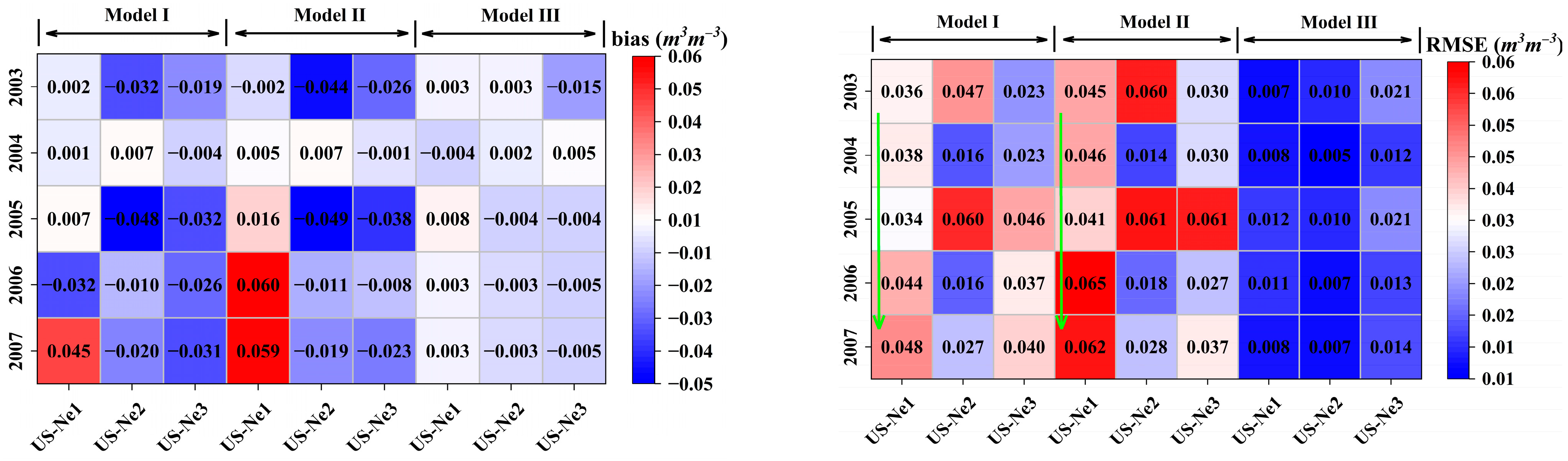
4.2. RZSM and ET Prediction with Different SHP Schemes

RZSM and ET in irrigated and rainfed croplands were derived with different SHP schemes to further understand the differences in their ability to predict water movement using HYDRUS-1D. To impartially evaluate the differences in the predicted results derived from the three SHP methods, the same historical data were used to obtain the SHPs for Models I, II, and III as mentioned in the previous section. For Models I and II, the l-parameter was set to 10 for Model I and II at all three sites, and systematic errors in 2002 for RZSM were recorded to calibrate the prediction results from 2003 to 2007. The heat maps of the accuracy of the RZSM and ET predictions from different SHP schemes are shown in Figure 10 and Figure 11, respectively. The average RMSE of the RZSM predictions in the three sites obtained using Models I, II, and III was 0.036 m³m⁻³, 0.042 m³m⁻³, and 0.011 m³m⁻³, respectively. Overall, the highest accuracy for an RZSM prediction was obtained for Model III, while comparable RZSM accuracies were also found for Models I and II. A large bias was generated based on Models I and II, resulting in less accurate prediction results. Moreover, the results indicated that the RZSM prediction accuracy decreased progressively in the continuous-Zea mays US-Ne1 field with the year based on Models I and II, which means that the error may be amplified over time under the same cover conditions. However, with Model III, the gradual decline in RZSM accuracy was not significant. From another perspective, it can be concluded that Model III can usually reduce systematic errors by optimizing more of the SHPs. Moreover, regular changes in accuracy were observed in the field with Zea mays–Glycine max rotation.

Owing to the high correlation between LE_EC and LE_EB, as shown in Figure 7, LE_EC was selected as the evaluation criterion. A minor difference in the RMSE of ET was found among the different SHP schemes, with an average RMSE of 66.4 Wm⁻² for Model I, 69.5 Wm⁻² for Model II, and 68.2 Wm⁻² for Model III. The reason for this result may be that ET derived from the P-M formula is mainly influenced by meteorological, water, and vegetation conditions. Under the same coverage conditions, a few rounds of irrigation may not cause large differences in ET. Nevertheless, a more reasonable bias was found in Model III. Similarly, ET prediction also decreased progressively in the continuous-Zea mays field US-Ne1 with the year based on Models I and II. The results showed that changes in the precision trends of ET and RZSM were consistent under different cover conditions in Models I and II.

SHPs from Model I and II are obtained using pedotransfert functions, but with errors that are sometimes significant due to sources of variability that cannot all be represented in stat functions established on soil databases. It is true that inverse methods (model III) give good results because all uncertainties are considered through the least-square method. In previous studies, the l-parameter was typically fixed at 0.5, but it was slightly adjusted using an iterative method to reduce errors in the present paper, which is one of the new aspects of this study. Overall, the accuracy of predicting RZSM and ET using the HYDRUS-1D model is comparable to previous studies [45]. Despite the divergent principles underpinning the three methodologies for the acquisition of SHPs, a common year was utilized for the calibration of all three at three geographically proximate sites. For Models I and II, the accuracy of the optimal prediction was obtained by adjusting the l-parameter and the systematic error. As for method III, all SHPs were derived by least-squares fitting, which integrates all factors affecting water transport. Overall, a comparative analysis of the results obtained from the prediction of ET using different SHPs reveals minimal variation. The accuracy of predicting RZSM using methods I and II is similar, while method III obtains the best accuracy. Although the three SHP schemes were calibrated using historical data, methods I and II adjusted only the l-parameter rather than all SHPs. The application of SHPs derived from PTFs to predict RZSM and ET may introduce substantial uncertainties, as statistical models developed from soil databases cannot comprehensively capture the inherent variability in these hydrological processes. On the other hand, method III faces challenges in generalizing the results to regional scales due to their reliance on site-specific calibration with field data, which is rarely available across large spatial extents.

4.3. RZSM and ET Prediction Under Different Crop and Moisture Conditions

As mentioned in the previous section, regular changes in accuracy were observed in the field with Zea mays–Glycine max rotation. The bias and RMSE in the Glycine max–Zea mays rotation fields (US-Ne2 and US-Ne3) were extracted for analysis of the various predicted results under different crop and moisture conditions, as shown in Figure 12 and Figure 13. The results showed that when SHPs in 2002 were applied to predict RZSM under different cover from 2003 to 2007, a reasonable accuracy was obtained under the same Glycine max cover, but an overall underestimation was observed under Zea mays cover. An almost unbiased result from different SHP schemes was observed under Glycine max cover. These results suggest that SHPs were affected by crop root structure and the water uptake model, resulting in systematic errors when the same SHP scheme was used. Notably, when using Model III, the RZSM predictions under different crop cover were more consistent. A plausible explanation is that Model III can reduce the transmission of errors because all effects are taken into account, compared with Models I and II. It is also clear from the RMSE results that the trend in accuracy was essentially consistent for the different SHP schemes at the same location. Reasonable accuracy was obtained for Glycine max, whereas unsatisfactory precision was obtained for Zea mays, especially when using Models I and II. The results indicate that when using SHPs based on soil information (Models I and II), systematic errors occur because of the influence of different crop root characteristics on soil structure. In summary, the three SHP methods both require historical data for calibration. Models I and II have the potential to be used on a large scale, but the impact of vegetation on water transportation should be taken into account, especially in arid areas.

The line graphs showing the bias and RMSE of ET in the Zea mays–Glycine max rotation field with different SHP schemes are provided in Figure 13. As can be seen from the bias results, the prediction of ET using HYDRUS-1D generally followed the pattern of RZSM in the US-Ne2 site under different cover conditions, where reasonable bias can be obtained for Glycine max, and high bias can be found for Zea mays. Notably, RZSM was undervalued overall, whereas ET was overvalued at the US-Ne2 site under Zea mays cover. In contrast to the US-Ne2 irrigation site, the US-Ne3 site is a rainfed field with frequent droughts during vegetation growth. At the US-Ne3 site, the bias in ET prediction did not vary with the bias in RZSM under different covers. In the irrigated field US-Ne2, the accuracy of the predicted ET generally followed the same pattern as that of the RZSM, where adequate RZSM led to stable ET. In terms of the water balance theory, when water consumption (i.e., ET) is overestimated, the RZSM will be underestimated. Moreover, for the rainfed field US-Ne3, inconsistent changes in the accuracy of predicting ET and RZSM were found due to changes in the ET response to RZSM as a result of the decrease in transpiration/ET under water stress. This indicates the decoupling of ET and RZSM in rainfed or arid cropland, which suggests that vegetation transpiration determines soil moisture–evapotranspiration coupling strength because transpiration is from RZSM. This finding contrasts with the study that surface soil moisture and evapotranspiration exhibit a stronger coupling in arid regions [67,68]. One potential explanation for this phenomenon is the role of RZSM as a buffer against drought. Moreover, new findings are presented in this study from the perspectives of RZSM and ET. When using SHP schemes based on soil information, the strength of the coupling between evapotranspiration and soil moisture is affected by different crop root characteristics on the soil structure, resulting in the decoupling of ET and RZSM.

5. Conclusions

A comprehensive assessment for predicting RZSM and ET by HYDRUS-1D using various SHP schemes under different crop and moisture conditions is carried out. Our findings provide suggestions for mapping ET and RZSM at the regional scale, and for research on the coupling strength of ET and soil moisture. Although all SHP schemes require historical data for calibration, the best accuracy of RZSM was obtained by the inverse solution scheme (RMSE = 0.011 m³m⁻³) once all the variability in these processes was considered. Meanwhile, the considerable accuracy of RZSM was found by the soil type-based (RMSE = 0.036 m³m⁻³) and soil texture-based (RMSE = 0.042 m³m⁻³) schemes. As for ET prediction, comparable accuracy was achieved with RMSEs of 66.4 Wm⁻², 69.5 Wm⁻², and 68.2 Wm⁻² from the three schemes. In the continuous-Zea mays field, the RZSM accuracy decreased over time by the three SHP schemes. However, systematic errors were dominated at the Zea mays–Glycine max rotation field. Based on our findings, vegetation causes a change in soil structure through the root system, which leads to error when using the SHP scheme based on soil information. This is useful for studies that use SHPs to estimate RZSM and evapotranspiration, as changes in land cover are not taken into further account after the calibration of the SHPs. Moreover, the accuracy variation of ET follows RZSM in the irrigation cropland but not in the rainfed cropland. This result indicates that the ET and RZSM are decoupled in arid areas due to the complex biophysical control of water transport in unsaturated environments. This finding contrasts with the study that surface soil moisture and evapotranspiration exhibit stronger coupling in arid regions. One potential explanation for this phenomenon is the role of RZSM as a buffer against drought.

References

1. Porter, J.R. Rising temperatures are likely to reduce crop yields. Nature 2005, 436, 174. [Google Scholar] [CrossRef] [PubMed]
2. Fritz, S.; See, L.; Mccallum, I.; You, L.; Bun, A.; Moltchanova, E.; Duerauer, M.; Albrecht, F.; Schill, C.; Perger, C.; et al. Mapping global cropland and field size. Glob. Change Biol. 2015, 21, 1980–1992. [Google Scholar] [CrossRef] [PubMed]
3. Potapov, P.; Turubanova, S.; Hansen, M.C.; Tyukavina, A.; Zalles, V.; Khan, A.; Song, X.P.; Pickens, A.; Shen, Q.; Cortez, J. Global maps of cropland extent and change show accelerated cropland expansion in the twenty-first century. Nat. Food 2022, 3, 19–28. [Google Scholar] [CrossRef]
4. Lesk, C.; Rowhani, P.; Ramankutty, N. Influence of extreme weather disasters on global crop production. Nature 2016, 529, 84–87. [Google Scholar] [CrossRef] [PubMed]
5. Schlenker, W.; Roberts, M.J. Nonlinear temperature effects indicate severe damages to us crop yields under climate change. Proc. Natl. Acad. Sci. USA 2009, 106, 15594–15598. [Google Scholar] [CrossRef]
6. Iizumi, T.; Furuya, J.; Shen, Z.; Kim, W.; Okada, M.; Fujimori, S.; Hasegawa, T.; Nishimori, M. Responses of crop yield growth to global temperature and socioeconomic changes. Sci. Rep. 2017, 7, 7800. [Google Scholar] [CrossRef]
7. Wang, E.; Martre, P.; Zhao, Z.; Ewert, F.; Maiorano, A.; Rötter, R.P.; Kimball, B.A.; Ottman, M.J.; Wall, G.W.; White, J.W. The uncertainty of crop yield projections is reduced by improved temperature response functions. Nat. Plants 2017, 3, 1–13. [Google Scholar]
8. Bodner, G.; Nakhforoosh, A.; Kaul, H. Management of crop water under drought: A review. Agron. Sustain. DEV Community 2015, 35, 401–442. [Google Scholar]
9. Dietz, K.J.; Zörb, C.; Geilfus, C.M. Drought and crop yield. Plant Biol. 2021, 23, 881–893. [Google Scholar] [CrossRef]
10. Li, Y.; Ye, W.; Wang, M.; Yan, X. Climate change and drought: A risk assessment of crop-yield impacts. Clim. Res. 2009, 39, 31–46. [Google Scholar] [CrossRef]
11. Boyer, J.S.; Byrne, P.; Cassman, K.G.; Cooper, M.; Delmer, D.; Greene, T.; Gruis, F.; Habben, J.; Hausmann, N.; Kenny, N.; et al. The U.S. drought of 2012 in perspective: A call to action. Glob. Food Secur. 2013, 2, 139–143. [Google Scholar] [CrossRef]
12. Hameed, M.; Ahmadalipour, A.; Moradkhani, H. Drought and food security in the middle east: An analytical framework. Agric. For. Meteorol. 2020, 281, 107816. [Google Scholar] [CrossRef]
13. Orimoloye, I.R. Agricultural drought and its potential impacts: Enabling decision-support for food security in vulnerable regions. Front. Sustain. Food Syst. 2022, 6, 838824. [Google Scholar] [CrossRef]
14. Huang, S.; Huang, Q.; Chang, J.; Leng, G.; Xing, L. The response of agricultural drought to meteorological drought and the influencing factors: A case study in the Wei River basin, China. Agric. Water Manag. 2015, 159, 45–54. [Google Scholar] [CrossRef]
15. Liu, X.; Zhu, X.; Pan, Y.; Li, S.; Liu, Y.; Ma, Y. Agricultural drought monitoring: Progress, challenges, and prospects. J. Geogr. Sci. 2016, 26, 750–767. [Google Scholar] [CrossRef]
16. Zhao, T.; Dai, A. Uncertainties in historical changes and future projections of drought. Part ii: Model-simulated historical and future drought changes. Clim. Change 2017, 144, 535–548. [Google Scholar]
17. Wang, F.; Lai, H.; Li, Y.; Feng, K.; Zhang, Z.; Tian, Q.; Zhu, X.; Yang, H. Dynamic variation of meteorological drought and its relationships with agricultural drought across China. Agric. Water Manag. 2022, 261, 107301. [Google Scholar] [CrossRef]
18. Howell, T.A. Enhancing water use efficiency in irrigated agriculture. Agron. J. 2001, 93, 281–289. [Google Scholar] [CrossRef]
19. Tao, F.; Yokozawa, M.; Hayashi, Y.; Lin, E. Changes in agricultural water demands and soil moisture in china over the last half-century and their effects on agricultural production. Agric. For. Meteorol. 2003, 118, 251–261. [Google Scholar] [CrossRef]
20. Liao, L.; Zhang, L.; Bengtsson, L. Soil moisture variation and water consumption of spring wheat and their effects on crop yield under drip irrigation. Irrig. Drain. Syst. 2008, 22, 253–270. [Google Scholar] [CrossRef]
21. Narasimhan, B.; Srinivasan, R. Development and evaluation of soil moisture deficit index (SMDI) and evapotranspiration deficit index (ETDI) for agricultural drought monitoring. Agric. For. Meteorol. 2005, 133, 69–88. [Google Scholar] [CrossRef]
22. Afshar, M.H.; Bulut, B.; Duzenli, E.; Amjad, M.; Yilmaz, M.T. Global spatiotemporal consistency between meteorological and soil moisture drought indices. Agric. For. Meteorol. 2022, 316, 108848. [Google Scholar] [CrossRef]
23. Touil, S.; Richa, A.; Fizir, M.; García, J.E.A.; Gómez, A.F.S. A review on smart irrigation management strategies and their effect on water savings and crop yield. Irrig. Drain. 2022, 71, 1396–1416. [Google Scholar] [CrossRef]
24. Jalilvand, E.; Abolafia Rosenzweig, R.; Tajrishy, M.; Kumar, S.V.; Mohammadi, M.R.; Das, N.N. Is it possible to quantify irrigation water-use by assimilating a high-resolution satellite soil moisture product? Water Resour. Res. 2023, 59, e2022WR033342. [Google Scholar] [CrossRef]
25. Zhuo, W.; Huang, H.; Gao, X.; Li, X.; Huang, J. An improved approach of winter wheat yield estimation by jointly assimilating remotely sensed leaf area index and soil moisture into the WOFOST model. Remote Sens. 2023, 15, 1825. [Google Scholar] [CrossRef]
26. Casa, R.; Rossi, M.; Sappa, G.; Trotta, A. Assessing crop water demand by remote sensing and GIS for the Pontina Plain, Central Italy. Water Resour. Manag. 2009, 23, 1685–1712. [Google Scholar] [CrossRef]
27. Ahmad, U.; Alvino, A.; Marino, S. A review of crop water stress assessment using remote sensing. Remote Sens. 2021, 13, 4155. [Google Scholar] [CrossRef]
28. Li, Z.L.; Leng, P.; Zhou, C.; Chen, K.S.; Zhou, F.C.; Shang, G.F. Soil moisture retrieval from remote sensing measurements: Current knowledge and directions for the future. Earth-Sci. Rev. 2021, 218, 103673. [Google Scholar] [CrossRef]
29. Jiménez, C.; Prigent, C.; Mueller, B.; Seneviratne, S.I.; McCabe, M.F.; Wood, E.F.; Rossow, W.B.; Balsamo, G.; Betts, A.K.; Dirmeyer, P.A.; et al. Global intercomparison of 12 land surface heat flux estimates. J. Geophys. Res. Atmos. 2011, 116, D02102. [Google Scholar] [CrossRef]
30. Xu, L.; Chen, N.C.; Zhang, X.; Moradkhani, H.; Zhang, C.; Hu, C. In-situ and triple-collocation based evaluations of eight global root zone soil moisture products. Remote Sens. Environ. 2021, 254, 112248. [Google Scholar] [CrossRef]
31. Yang, F.; White, M.A.; Michaelis, A.R.; Ichii, K.; Hashimoto, H.; Votava, P.; Zhu, A.X.; Nemani, R.R. Prediction of continental-scale evapotranspiration by combining MODIS and Ameriflux data through support vector machine. IEEE Trans. Geosci. Remote Sens. 2006, 44, 3452–3461. [Google Scholar] [CrossRef]
32. Ahmad, S.; Kalra, A.; Stephen, H. Estimating soil moisture using remote sensing data: A machine learning approach. Adv. Water Resour. 2010, 33, 69–80. [Google Scholar] [CrossRef]
33. Ali, I.; Greifeneder, F.; Stamenkovic, J.; Neumann, M.; Notarnicola, C. Review of machine learning approaches for biomass and soil moisture retrievals from remote sensing data. Remote Sens. 2015, 7, 16398–16421. [Google Scholar] [CrossRef]
34. Guswa, A.J.; Celia, M.A.; Rodriguez-Iturbe, I. Models of soil moisture dynamics in ecohydrology: A comparative study. Water Resour. Res. 2002, 38, 1–5. [Google Scholar] [CrossRef]
35. Šimůnek, J.; Van Genuchten, M.T.; Sejna, M. The hydrus-1d software package for simulating the one-dimensional movement of water, heat, and multiple solutes in variably-saturated media. Univ. Calif.-Riverside Res. Rep. 2005, 3, 1–240. [Google Scholar]
36. Jones, J.W.; Hoogenboom, G.; Porter, C.H.; Boote, K.J.; Batchelor, W.D.; Hunt, L.A.; Wilkens, P.W.; Singh, U.; Gijsman, A.J.; Ritchie, J.T. The DSSAT cropping system model. Eur. J. Agron. 2003, 18, 235–265. [Google Scholar] [CrossRef]
37. Keating, B.A.; Carberry, P.S.; Hammer, G.L.; Probert, M.E.; Robertson, M.J.; Holzworth, D.; Huth, N.I.; Hargreaves, J.N.; Meinke, H.; Hochman, Z.; et al. An overview of APSIM, a model designed for farming systems simulation. Eur. J. Agron. 2003, 18, 267–288. [Google Scholar] [CrossRef]
38. Steduto, P.; Hsiao, T.C.; Raes, D.; Fereres, E. AquaCrop—The FAO crop model to simulate yield response to water: I. Concepts and underlying principles. Agron. J. 2009, 101, 426–437. [Google Scholar] [CrossRef]
39. Šimůnek, J.; van Genuchten, M.T.; Aejna, M. Recent developments and applications of the HYDRUS computer software packages. Vadose Zone J. 2016, 15, 1–25. [Google Scholar] [CrossRef]
40. Han, M.; Zhao, C.; Šimůnek, J.; Feng, G. Evaluating the impact of groundwater on cotton growth and root zone water balance using hydrus-1d coupled with a crop growth model. Agric. Water Manag. 2015, 160, 64–75. [Google Scholar] [CrossRef]
41. Li, Y.; Šimůnek, J.; Jing, L.; Zhang, Z.; Ni, L. Evaluation of water movement and water losses in a direct-seeded-rice field experiment using hydrus-1d. Agric. Water Manag. 2014, 142, 38–46. [Google Scholar] [CrossRef]
42. Sahaar, S.A.; Niemann, J.D. Impact of regional characteristics on the estimation of root-zone soil moisture from the evaporative index or evaporative fraction. Agric. Water Manag. 2020, 238, 106225. [Google Scholar] [CrossRef]
43. Sahaar, S.A.; Niemann, J.D.; Elhaddad, A. Using regional characteristics to improve uncalibrated estimation of root-zone soil moisture from optical/thermal remote-sensing. Remote Sens. Environ. 2022, 273, 112982. [Google Scholar] [CrossRef]
44. Shelia, V.; Šimůnek, J.; Boote, K.; Hoogenbooom, G. Coupling DSSAT and hydrus-1d for simulations of soil water dynamics in the soil-plant-atmosphere system. J. Hydrol. Hydromech. 2018, 66, 232–245. [Google Scholar] [CrossRef]
45. Yu, J.; Wu, Y.; Xu, L.; Peng, J.; Chen, G.; Shen, X.; Lan, R.; Zhao, C.; Zhangzhong, L. Evaluating the hydrus-1d model optimized by remote sensing data for soil moisture simulations in the maize root zone. Remote Sens. 2022, 14, 6079. [Google Scholar] [CrossRef]
46. Feng, H.; Wu, Z.; Dong, J.; Zhou, J.; Brocca, L.; He, H. Transpiration–Soil evaporation partitioning determines inter-model differences in soil moisture and evapotranspiration coupling. Remote Sens. Environ. 2023, 298, 113841. [Google Scholar] [CrossRef]
47. Mahmood, R.; Hubbard, K.G. Assessing bias in evapotranspiration and soil moisture estimates due to the use of modeled solar radiation and dew point temperature data. Agric. For. Meteorol. 2005, 130, 71–84. [Google Scholar] [CrossRef]
48. Suyker, A.E.; Verma, S.B.; Burba, G.G.; Arkebauer, T.J. Gross primary production and ecosystem respiration of irrigated maize and irrigated soybean during a growing season. Agric. For. Meteorol. 2005, 131, 180–190. [Google Scholar] [CrossRef]
49. Suyker, A.E.; Verma, S.B.; Burba, G.G.; Arkebauer, T.J.; Walters, D.T.; Hubbard, K.G. Growing season carbon dioxide exchange in irrigated and rainfed maize. Agric. For. Meteorol. 2004, 124, 1–13. [Google Scholar] [CrossRef]
50. Xing, Z.; Fan, L.; Zhao, L.; De Lannoy, G.; Frappart, F.; Peng, J.; Li, X.; Zeng, J.; Al-Yaari, A.; Yang, K.; et al. A first assessment of satellite and reanalysis estimates of surface and root-zone soil moisture over the permafrost region of Qinghai-Tibet Plateau. Remote Sens. Environ. 2021, 265, 112666. [Google Scholar] [CrossRef]
51. Richards, L.A. Capillary conduction of liquids through porous mediums. Physics 1931, 1, 318–333. [Google Scholar] [CrossRef]
52. Van Genuchten, M.T. A closed-form equation for predicting the hydraulic conductivity of unsaturated soils. Soil Sci. Soc. Am. J. 1980, 44, 892–898. [Google Scholar] [CrossRef]
53. Monteith, J.L. Evaporation and environment. In Symposia of the Society for Experimental Biology; Cambridge University Press (CUP) Cambridge: Cambridge, UK, 1965; Volume 19, pp. 205–234. [Google Scholar]
54. Allen, R.G.; Pereira, L.S.; Raes, D.; Smith, M. Crop evapotranspiration-guidelines for computing crop water requirements-FAO irrigation and drainage paper 56. FAO Rome 1998, 300, D05109. [Google Scholar]
55. Carsel, R.F.; Parrish, R.S. Developing joint probability distributions of soil water retention characteristics. Water Resour. Res. 1988, 24, 755–769. [Google Scholar] [CrossRef]
56. Mualem, Y. A new model for predicting the hydraulic conductivity of unsaturated porous media. Water Resour. Res. 1976, 12, 513–522. [Google Scholar] [CrossRef]
57. Schaap, M.G.; Leij, F.J. Improved prediction of unsaturated hydraulic conductivity with the Mualem-van Genuchten model. Soil Sci. Soc. Am. J. 2000, 64, 843–851. [Google Scholar] [CrossRef]
58. Kaufmann, K.W. Fitting and using growth curves. Oecologia 1981, 49, 293–299. [Google Scholar] [CrossRef] [PubMed]
59. Sun, S.; Frelich, L.E. Flowering phenology and height growth pattern are associated with maximum plant height, relative growth rate and stem tissue mass density in herbaceous grassland species. J. Ecol. 2011, 99, 991–1000. [Google Scholar] [CrossRef]
60. Xiao, Z.; Liang, S.; Wang, J.; Xiang, Y.; Zhao, X.; Song, J. Long-time-series global land surface satellite leaf area index product derived from MODIS and AVHRR surface reflectance. IEEE Trans. Geosci. Remote Sens. 2016, 54, 5301–5318. [Google Scholar] [CrossRef]
61. Bolton, D.K.; Friedl, M.A. Forecasting crop yield using remotely sensed vegetation indices and crop phenology metrics. Agric. For. Meteorol. 2013, 173, 74–84. [Google Scholar] [CrossRef]
62. De Boor, C. A practical guide to splines. Appl. Math. Sci. 1978, 27, 325. [Google Scholar]
63. Ordóñez, R.A.; Castellano, M.J.; Hatfield, J.L.; Helmers, M.J.; Licht, M.A.; Liebman, M.; Dietzel, R.; Martinez-Feria, R.; Iqbal, J.; Puntel, L.A.; et al. Maize and soybean root front velocity and maximum depth in Iowa, USA. Field Crops Res. 2018, 215, 122–131. [Google Scholar] [CrossRef]
64. Andersen, J.; Dybkjaer, G.; Jensen, K.H.; Refsgaard, J.C.; Rasmussen, K. Use of remotely sensed precipitation and leaf area index in a distributed hydrological model. J. Hydrol. 2022, 264, 34–50. [Google Scholar] [CrossRef]
65. Schaap, M.G.; Leij, F.J.; van Genuchten, M.T. ROSETTA: A computer program for estimating soil hydraulic parameters with hierarchical pedotransfer functions. J. Hydrol. 2001, 251, 163–176. [Google Scholar] [CrossRef]
66. Feng, G.; Zhu, C.; Wu, Q.; Wang, C.; Zhang, Z.; Mwiya, R.M.; Zhang, L. Evaluating the impacts of saline water irrigation on soil water-salt and summer maize yield in subsurface drainage condition using coupled HYDRUS and EPIC model. Agric. Water Manag. 2021, 258, 107175. [Google Scholar] [CrossRef]
67. Dong, J.; Dirmeyer, P.A.; Lei, F.; Anderson, M.C.; Holmes, T.R.H.; Hain, C.; Crow, W.T. Soil evaporation stress determines soil moisture–evapotranspiration coupling strength in land surface modeling. Geophys. Res. Lett. 2020, 47, e2020GL090391. [Google Scholar] [CrossRef]
68. Seneviratne, S.I.; Corti, T.; Davin, E.L.; Hirschi, M.; Jaeger, E.B.; Lehner, I.; Orlowsky, B.; Teuling, A.J. Investigating soil moisture-climate interactions in a changing climate: A review. Earth-Sci. Rev. 2010, 99, 125–161. [Google Scholar] [CrossRef]
Figure 1. View and locations of study sites in present investigation. (US-Ne1 and US-Ne2 are irrigated fields. US-Ne3 is a rainfed field).
Water 17 00730 g001
Figure 2. Fitting results for RZSM based on least-square theory using the Model III scheme.
Water 17 00730 g002
Figure 3. Calibration of vegetation parameters and irrigation/precipitation in US-Ne1.
Water 17 00730 g003
Figure 4. Calibration of vegetation parameters and irrigation/precipitation in US-Ne2.
Water 17 00730 g004
Figure 5. Calibration of vegetation parameters and precipitation in US-Ne3.
Water 17 00730 g005
Figure 6. Scatter plot and time-varying line charts of the predicted and measured RZSM.
Water 17 00730 g006
Figure 7. Scatter plot and time-varying line charts of predicted and measured ET.
Water 17 00730 g007aWater 17 00730 g007b
Figure 8. Scatterplot between predicted and measured RZSM, predicted and measured ET in US-Ne3.
Water 17 00730 g008aWater 17 00730 g008b
Figure 9. Accuracy of the dotted-line plots vary with l-parameter ((a,b) are the patterns of RZSM and ET accuracy predicted by Model I, respectively; (c,d) are the patterns of RZSM and ET accuracy predicted by Model II, respectively).
Water 17 00730 g009
Figure 10. Accuracy of the heatmaps of RZSM predicted with different SHP schemes.
Water 17 00730 g010
Figure 11. Accuracy of the heatmaps of ET prediction with different SHP schemes.
Water 17 00730 g011
Figure 12. Line graph of bias and RMSE of RZSM over Zea maysGlycine max rotation field with different SHP schemes.
Water 17 00730 g012
Figure 13. Line graph of bias and RMSE of ET over Zea maysGlycine max rotation field with different SHP schemes.
Water 17 00730 g013