Drag Force and Heat Transfer Characteristics of Ellipsoidal Particles near the Wall

Abstract

This study investigates the force and heat transfer characteristics of oblate spheroidal particles in gas–solid two-phase flows near walls, addressing the influence of particle orientation, shape, Reynolds number, and particle–wall distance. These factors are critical in industrial processes such as pneumatic transport and crop drying, as well as in natural phenomena. Utilizing the Euler–Lagrangian model and large eddy simulation (LES), we simulated flow fields and heat transfer under various conditions. The results indicate that at Re = 500, turbulence mitigates wall interference, leading to a 14.4% increase in the Nusselt number (Nu). Particle orientation plays a crucial role in heat transfer, with Nu decreasing by 20% at = 90° due to restricted interstitial flow. A higher aspect ratio (Ar = 0.8) enhances heat transfer by 25% compared to a lower aspect ratio (Ar = 0.1). Additionally, increasing the particle–wall distance from H = 0.25$d_v$ to H = 0.5$d_v$ reduces wall-induced drag by 30%. The findings enhance the understanding of particle–fluid interactions near walls, providing a foundation for optimizing computational fluid dynamics models and improving industrial applications. Future work should consider additional variables such as particle roughness to further refine predictive capabilities. This study contributes to advancing theoretical and practical insights into non-spherical particle behaviors in complex flow environments.

1. Introduction

Granular flow is the shear flow of a large number of granular materials, which can be regarded as a special gas (or liquid)–solid two-phase flow. This flow phenomenon involves a wide range of problems in nature and engineering, such as avalanches [1], landslides [2], debris flows [3], and the lamination movement of coarse particles at the bottom of rivers, as well as the pipeline transportation of solid materials in industry [4], fluidized beds in food processing [5], chemical engineering [6], etc.

In the past few decades, the study of particles has mainly focused on understanding the flow mechanism of particles, the most important of which is the study of particle–fluid interaction, which involves complex momentum and heat transfer [7]. However, due to the complexity of particle flow, experimental studies are not always able to accurately describe the basic characteristics of particles or completely explain the related phenomena. In recent years, with the improvement of computer computing power, the use of computers for numerical calculation has been adopted by more and more researchers. Motlagh and Hashemabadi [8] used the standard $k-\epsilon$ turbulence model to simulate the two different arrangements of particles in a packed-bed 3D CFD, which was verified by naphthalene sublimation mass transfer experiments. They found that CFD (computational fluid dynamics) can be used to discuss momentum and heat transfer in fluid particles. With the gradual improvement of computational fluid dynamics, more and more numerical simulation models of particle–fluid interaction are gradually improved, such as the Euler–Lagrangian model (Euler–Lagrange) [9,10], Euler–Euler model (Euler–Euler) [11,12], and so on. With the help of these models, researchers can easily study and analyze fluid–particle flow. The pros and cons of these models have been discussed in some references [13,14]. Only by providing the closed relationship of the interaction between particles and fluid can these models be used more accurately, in which the Drag coefficient ($c_d$) and Nusselt number (Nu) are the more important closed relations [15]. Therefore, it is very important to obtain accurate drag coefficients and Nusselt numbers for the study of fluid–particle flow.

Because the geometric structure of spherical particles is relatively simple, the research on spherical particles is quite rich [16,17,18,19]. A large number of related data and expressions of the drag coefficient and Nusselt number with high prediction accuracy have been published in the literature [20]. These studies on spherical particles improve the accuracy of the Euler–Lagrangian model, and researchers can carry out the study of the particle–fluid coupling flow of spherical particles at low cost. But in fact, most non-spherical particles are mostly encountered in nature and industrial applications [21], such as pollen transport [22], biomass energy, blood flow [23], powdered solid fuel transport [24], etc. Different from the sphere, the characteristic length of non-spherical particles cannot be regarded as a single scale of a dimensionless number. Therefore, the spherical particle closure relationship previously established is not suitable for non-spherical particles [25]. Through experimental research, Roos et al. [26] found that the asphericity of particles has great influence on the fluid–particle interaction, thus affecting the motion of particles. The research on the drag force and heat transfer of non-spherical particles is theoretically conducive to improving the cognition of the actual particle flow, and from a practical application, it is conducive to improving the simulation accuracy of the actual situation. For example, it is beneficial to optimize the heat transfer of particle flow in a moving bed heat exchanger [27], better understand the heat transfer characteristics of supercritical water and solid particles in new energy developments [28], improve computational fluid dynamics simulations, such as of aircraft and submarine design [29], and so on.

Non-spherical particles come in a variety of shapes and sizes, such as ellipsoids, cylinders, disks, and other irregular shapes. Hottovy and Sylvester [30] studied the settlement of 12 irregularly shaped particles and found that the drag coefficient was higher than that of spherical particles when Re ranged from 100 to 3000. Similarly to Hottovy, some researchers have also determined the drag coefficient of irregular particle settlement through experiments [31,32,33,34]. It is impossible to study all kinds of particles. At present, scholars usually simplify the particles and then carry out numerical simulations. They are usually modeled as fibers, cylinders, or ellipsoids. The smoothness and symmetry of ellipsoids make it a hot spot in analysis and numerical research [35]. Many researchers have conducted in-depth studies based on the drag coefficients [36,37] and heat transfer models proposed by predecessors. Holzer and Sommerfeld [38] established a drag correlation for arbitrarily shaped particles. Richter and Nikrityuk [39] conducted numerical simulations of cuboid, spherical, and ellipsoid particles within Re from 10 to 250. They found that the drag coefficient depends on the normalized longitudinal length, while both the sphericity and the crosswise sphericity influence the Nusselt number. Rong and Zhou [40] studied the flow in a uniform ellipsoidal packed bed and put forward a new formula for calculating the drag force. Sanjeevi et al. [41] carried out the numerical simulation of oblate spheroidal particles using the Lattice Boltzmann method, and obtained the expressions of the drag coefficient, lift coefficient, and Nusselt number of oblate spheroids. At the same time, it was also found that the drag coefficient of oblate spheroids varied with particle orientation, and the lift coefficient of slender particles changed. Ke et al. [42] studied the heat transfer characteristics of particles by introducing particle orientation in the range. It was found that the Nusselt number varies with the orientation of the particles. The above studies do not consider the influence of the wall on the particle flow characteristics, but in fact, the wall will affect the relationship between the orientation of the particles near the wall and the drag force. In addition, some researchers have begun to focus on the particle characteristics near the wall. Mirhashemi [43] carried out numerical and experimental studies on the heat transfer of single cylindrical particles affected by the wall surface and proposed a CFD correlation method considering the influence of the wall effect on the particle–fluid Nusselt number. EL Hasadi and Padding [44] demonstrated that the fluid drag felt by ellipsoidal and spherical cylindrical particles can be predicted with machine learning methods, and a new set of drag relations were proposed. Toghraie [45] and others used numerical simulation to study the heat transfer of spherical particles arranged in series, the heat transfer of three-lobe particles on the wall, and the Nusselt number. Zare [46] et al. studied the effect of a wall on the heat transfer of non-spherical particles using experimental methods and numerical simulation, in which the effects of the tube wall, particle shape, and particle rotation angle on the formation of the heat transfer zone were tested in detail.

At present, some progress has been made in the study of the force and heat transfer characteristics of prolate spheroidal particles in uniform flow, but relatively few studies have been conducted on near-wall ellipsoids. In view of this, the drag and heat transfer characteristics of oblate spheroids near the wall were studied in this work in order to clarify the influence mechanism of particle shape, particle orientation, and wall conditions on the drag and heat transfer characteristics of particles. The Euler–Lagrangian model of the gas–solid heat transfer of oblate spheroids was optimized to provide guidance for industrial applications involving particle–fluid interaction (pneumatic transport, crop drying, etc.) and natural environment research.

2. Research Method

2.1. Large Eddy Simulation

Turbulence is a complex fluid flow state characterized by irregularity, multi-scale interactions, and nonlinear transport. Experimental studies of turbulence are costly, making numerical simulations a preferred alternative due to their lower cost and higher precision. Turbulence modeling methods include Direct Numerical Simulation (DNS), large eddy simulation (LES), and Reynolds-averaged Navier–Stokes (RANS). DNS directly solves governing equations without requiring closure models but demands extremely fine grids to resolve all turbulence scales. Computational costs for DNS scale cubically with the turbulent Reynolds number, rendering it impractical for high Reynolds number flows in engineering applications due to excessive memory and CPU requirements. The RANS method describes fluid flow using equations based on fundamental physical laws, with the Navier–Stokes equation at its core to solve time-averaged values. Physical quantities are decomposed into the mean time and fluctuating components, with the mean values solved directly and the effects of fluctuations modeled. However, no single turbulence model suits all flow conditions, and results can vary between models under identical conditions, requiring users to apply experience and judgment.

LES combines the strengths of DNS [47,48,49,50] and RANS [51,52,53,54] by dividing turbulence into large and small eddies. Large eddies correspond to the characteristic length of the mean flow, while small eddies handle turbulent kinetic energy dissipation. This separation assumes minimal impact between scales. LES solves high-precision, three-dimensional instantaneous flow equations for large eddies, while small eddies are modeled, reducing the need for fine grids and small time steps. The key principles of LES are the following: (1) Large eddies transport most of the momentum, mass, energy, and other scalars. (2) Large eddies depend on flow geometry and boundary conditions. (3) Small eddies are largely isotropic and less geometry-dependent. (4) General turbulence models are more applicable to small eddies.

Large-scale eddies play a crucial role in turbulent flow, making LES more effective than general turbulence models for accurate predictions. LES focuses on larger eddies, allowing for coarser grids and larger time steps compared to DNS, though finer than those in RANS. Computationally, LES is less demanding than DNS but more intensive than RANS. Unlike RANS, which relies on complete modeling and empirical parameterization (e.g., Reynolds stress), LES offers greater accuracy. Advances in computational power have made LES increasingly viable for industrial applications.

2.2. Control Equation

The three-dimensional incompressible continuity equation, momentum equation, and energy equation can be expressed as follows:

$${\displaystyle \frac{\partial \overline{u_i}}{\partial x_i}}=0$$

(1)

$${\displaystyle \frac{\partial }{\partial t}}(\rho \overline{u_i})+{\displaystyle \frac{\partial }{\partial x_j}}(\rho \overline{u_i}\overline{u_j})=-{\displaystyle \frac{\partial \overline{p}}{\partial x_i}}+{\displaystyle \frac{\partial }{\partial x_j}}(\mu {\displaystyle \frac{\partial \overline{u_i}}{\partial x_j}})-{\displaystyle \frac{\partial {\tau }_{ij}}{\partial x_j}}$$

(2)

$$\rho c_p{\displaystyle \frac{\partial \overline{T}}{\partial t}}+\rho c_p\overline{u_j}{\displaystyle \frac{\partial \overline{T}}{\partial x_j}}={\displaystyle \frac{\partial }{\partial x_j}}\left((k+k_t){\displaystyle \frac{\partial \overline{T}}{\partial x_j}}\right)$$

(3)

In the above formulas, $\overline{u_i}$ is the filtered motion speed, where $i$ represents the component of the velocity in the $i$ direction; $\rho$ is the fluid density in kg/m³; $\overline{p}$ is the pressure after filtration in Pa; $\overline{T}$ is the filtered temperature in K; $c_p$ is the specific heat capacity of the fluid in J/(kg·°C); and $k$ is the thermal conductivity of the fluid in w/(m·k). $k_t$ is the turbulent thermal conductivity, and its calculation expression is as follows:

$$k_t={\displaystyle \frac{{\mu }_t{c}_p}{Pr}}$$

(4)

$${\mu }_t=C_d{\Delta }^2\left|\overline{S}\right|$$

(5)

$${\Delta }^2=(\Delta x_1^2+\Delta x_2^2+\Delta x_3^2)$$

(6)

$$\left|\overline{S}\right|={(2\overline{S_{ij}}\overline{S_{ij}})}^{1/2}$$

(7)

$C_d$ in the above formula is the dynamic Smagorinsky coefficient, which is calculated using the least squares method, and $Pr$ is the Prandtl number. Its definition and value will be introduced later.

In this study, the wall adaptive local eddy viscosity model (Wall-Adapting Local Eddy viscosity Model, WALE) was used as the large eddy simulation subgrid model [39]. ${\tau }_{ij}$ is the subgrid stress, which is defined as

$${\tau }_{ij}=\overline{u_i{u}_j}-\overline{u_i}\overline{u_j}$$

(8)

It is based on the eddy viscosity hypothesis.

$${\tau }_{ij}-{\displaystyle \frac{1}{3}}{\delta }_{ij}{\tau }_{kk}=2v_t\overline{S_{ij}}$$

(9)

$$\overline{S_{ij}}={\displaystyle \frac{1}{2}}({\displaystyle \frac{\partial \overline{u_i}}{\partial x_j}}+{\displaystyle \frac{\partial \overline{u_j}}{\partial x_i}})$$

(10)

The eddy current viscosity $v_t$ is calculated as follows:

$${v_t=L_s}^2{\displaystyle \frac{{(S_{ij}^d{S}_{ij}^d)}^{3/2}}{{(S_{ij}{S}_{ij})}^{5/2}+{(S_{ij}^d{S}_{ij}^d)}^{5/4}}}$$

(11)

$$L_s=\min (k_{v}r,C_w{V}^{1/3})$$

(12)

$k_v$ is the Von Kármán constant with a value of 0.41; $C_w$ is the WALE constant problem description with a value of 0.325; $r$ is the nearest distance to the wall; $V$ is the volume of the calculation unit; and $S_{ij}^d$ is the unscented symmetric tensor of the square of the velocity gradient tensor.

$$S_{ij}^d={\displaystyle \frac{1}{2}}({\displaystyle \frac{\partial \overline{u_i}}{\partial x_k}}{\displaystyle \frac{\partial \overline{u_k}}{\partial x_j}}+{\displaystyle \frac{\partial \overline{u_j}}{\partial x_k}}{\displaystyle \frac{\partial \overline{u_k}}{\partial x_i}})-{\displaystyle \frac{1}{3}}{\delta }_{ij}{\displaystyle \frac{\partial \overline{u_l}}{\partial x_k}}{\displaystyle \frac{\partial \overline{u_k}}{\partial x_l}}$$

(13)

2.3. Dimensionless Parameter

The Reynolds number (Re) is a dimensionless parameter used to characterize fluid flow. It is defined based on the volume-equivalent diameter of the prolate spheroid ($d_v$) and the inlet fluid velocity ($\left|\overrightarrow{V}\right|$).

$$Re={\displaystyle \frac{\left|\overrightarrow{V}\right|d_v}{\nu }}$$

(14)

$\nu$ is the kinematic viscosity of the fluid, with units of m²/s. The volume-equivalent diameter ($d_v$) of all spheroids is 10 mm.

The Prandtl number (Pr) is a dimensionless parameter that characterizes the interplay between energy and momentum transport in a fluid. Its value remains constant at 0.744. The calculation methods for the drag coefficient and Nusselt number are as follows:

$$c_d={\displaystyle \frac{8\left|{\overrightarrow{F}}_d\right|}{\rho \pi d_v^2{U}^2}}$$

(15)

$$Nu={\displaystyle \frac{d_v}{(T_p-T_f)S_p}}{\displaystyle \underset{S_p}{\int }\nabla T_f\cdot \overrightarrow{n}dS}$$

(16)

${\overrightarrow{F}}_d$ is the particle drag force, with units of N. $T_p$ and $T_f$ are the particle surface temperature and fluid temperature, respectively, with units of K. $\rho$ is the fluid density, with units of kg/m³. $S_p$ represents the particle surface area, with units of m².

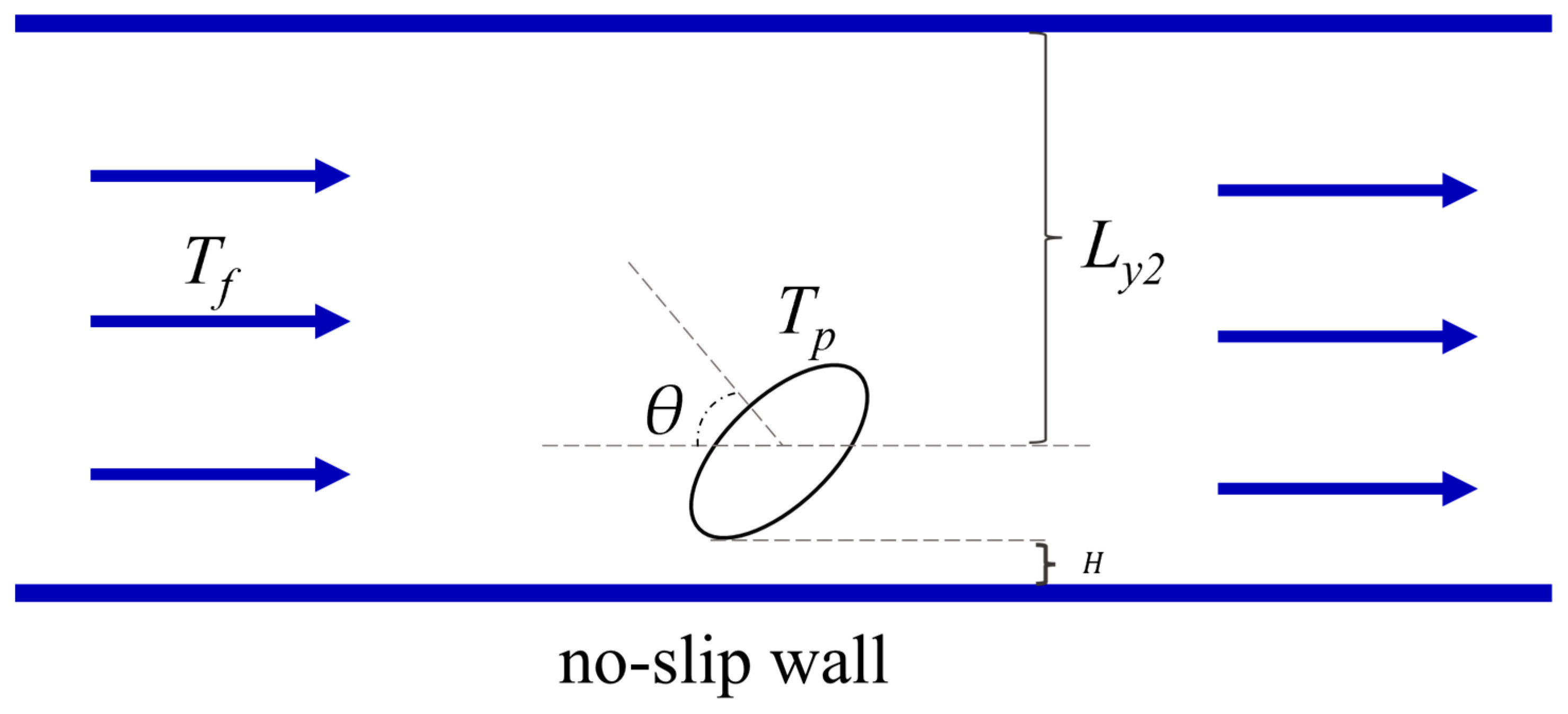
2.4. The Governing Equation and Simulation Parameters

All numerical simulations in this study were conducted using the software ANSYS Fluent 2021 R2. In addition to the Reynolds number (Re), particle orientation (θ), and aspect ratio (Ar), the particle–wall distance (H) was introduced to examine its impact on particle force and heat transfer near a wall. This study investigated the effects of these parameters on the drag force and heat transfer characteristics of single-static, constant-temperature oblate spheroids in gas–solid two-phase flow near a wall. Key parameters included the following: $Re=$ 50, 100, 200, 500; $H$ = 0.25$d_v$, 0.5$d_v$, $d_v$; $d_v=10 \mathrm{m}\mathrm{m}$; Ar = 0.1, 0.5, 0.8; $\theta =$0$°$, 30$°$, 60$°$, 90$°$, 120$°$, 150$°$, 180$°$; $Pr=$ 0.744. It should be pointed out that in the range of the Reynolds number, the turbulence model was used to simulate the flow field.

The governing equation of the ellipsoid is as follows:

$${\left({\displaystyle \frac{x}{a}}\right)}^2+{\left({\displaystyle \frac{y}{b}}\right)}^2+{\left({\displaystyle \frac{z}{c}}\right)}^2=1$$

(17)

In the given formula, a, b, and c represent the half-axes of the particle, with c as the rotation axis and a = b as the long half-axes. The aspect ratio (Ar) of an ellipsoid is defined as the ratio of the rotation axis to the long axis (Ar = c/a). For oblate spheroid particles, Ar is the ratio of the rotation axis to the short axis. The particle orientation (θ) refers to the angle between the rotation axis and the fluid flow direction, as illustrated in Figure 1, where the dotted line denotes the ellipsoid’s rotation axis.

2.5. Setting of Boundary Conditions

As shown in Figure 2, the computational domain for the oblate spheroidal particles near the wall is rectangular, with the particle positioned close to the bottom wall. The shortest distance between the particle’s lower surface and the wall is denoted as H. Fluid enters from the inlet on the left, flows over static, constant-temperature oblate spheroidal particles, and exits through the outlet on the right. The center of the particle remains at a constant distance L_y2 from the domain’s upper boundary. The inlet velocity is specified, with an inflow temperature of 200 K. The particle surface is modeled as a no-slip wall at a constant temperature of 300 K. The bottom wall is also no-slip but is thermally insulated to prevent heat exchange with the fluid. Other boundaries are set as symmetric, and the outlet is under an outflow condition. (The outflow boundary condition assumes that the flow at the outlet is fully developed, that is, the gradient of flow variables (such as velocity and pressure) in the normal direction of the outlet is zero.) This model enables a detailed study of wall effects on the fluid heat transfer process.

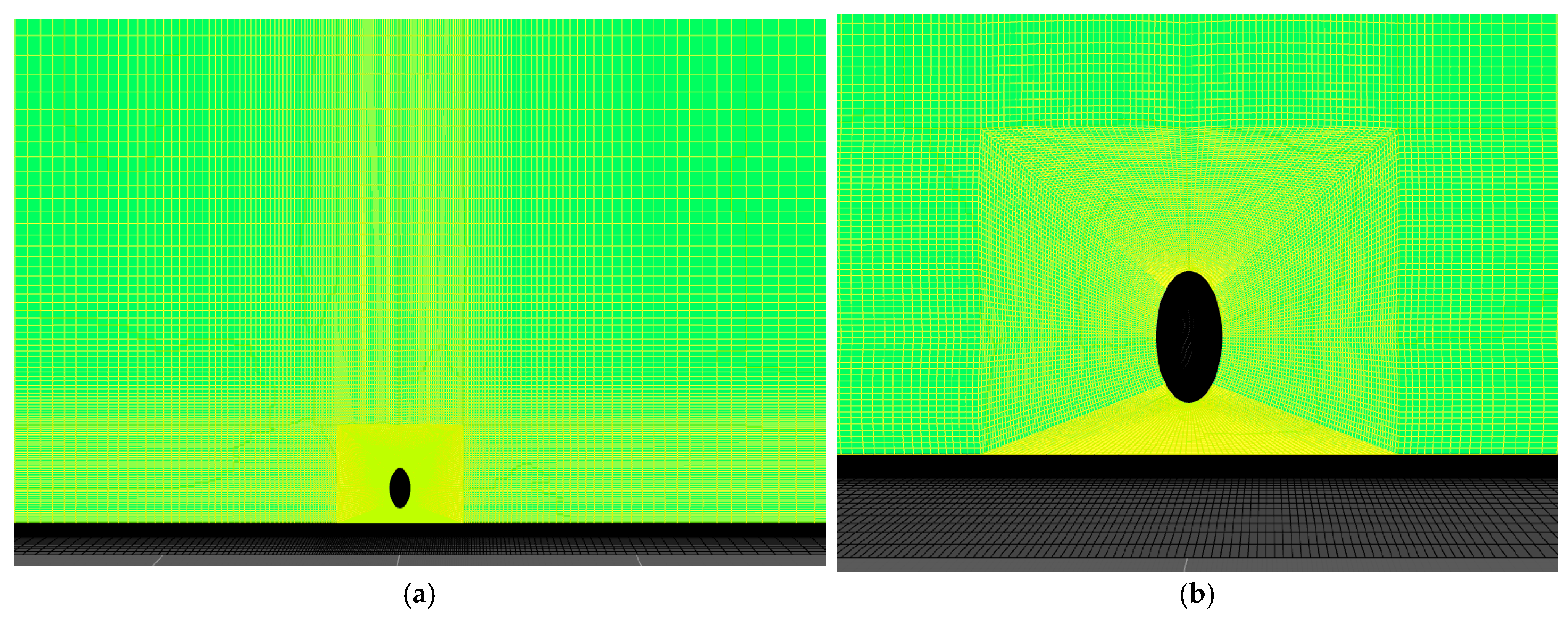
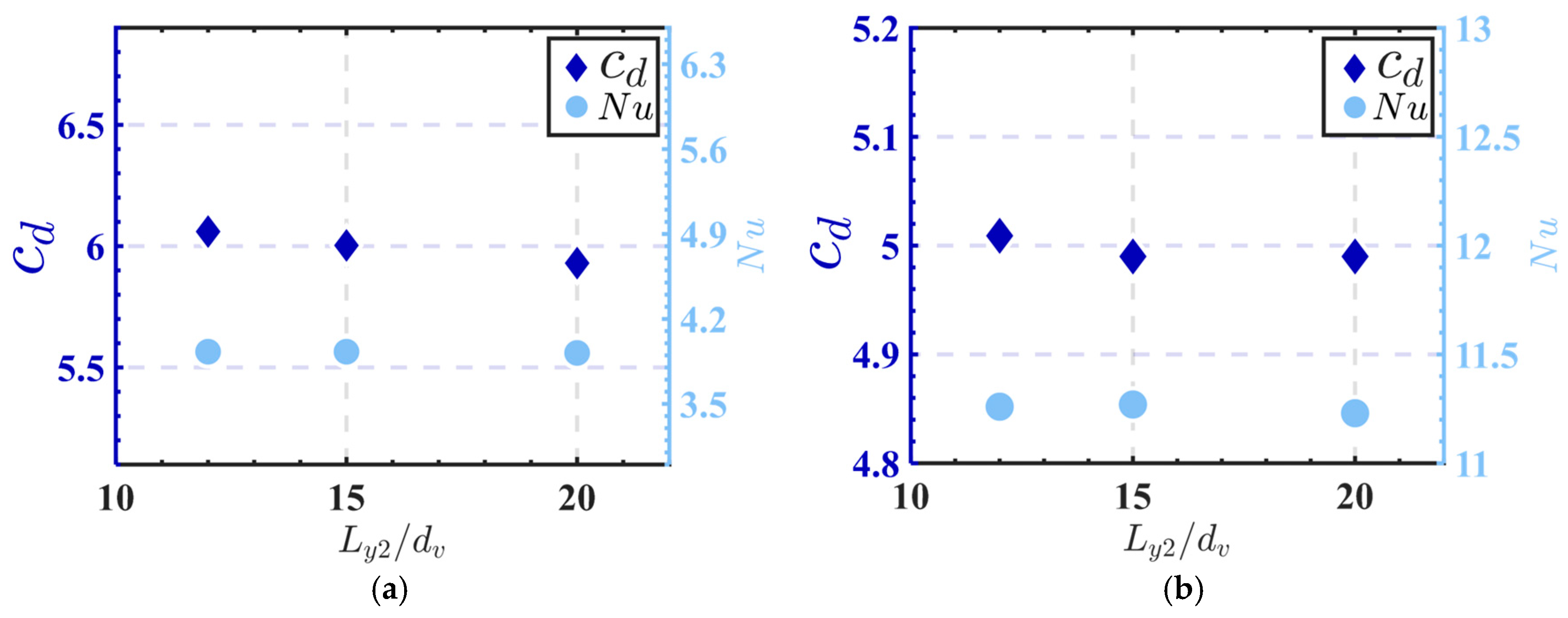
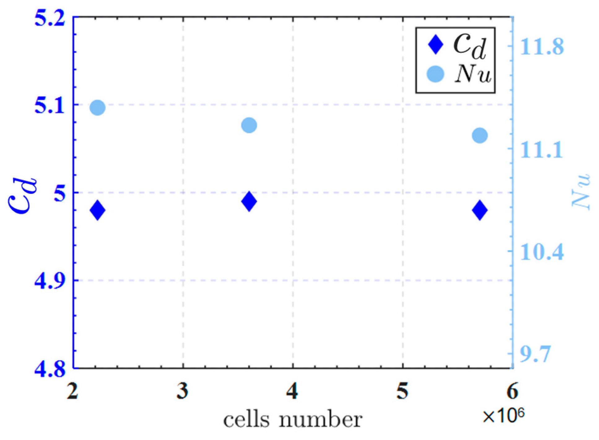
2.6. Meshing and Grid Independence Verification

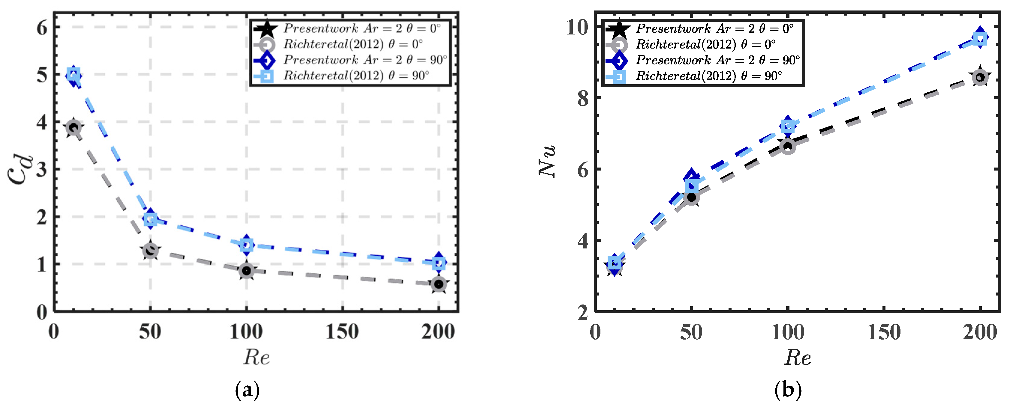
The gas–solid heat transfer model grid for a near-wall oblate spheroid is shown in Figure 3. The fluid domain was meshed using ICEM with a consistent hexahedral meshing method across all cases. To ensure accurate numerical results, the particle surface was modeled as a no-slip wall, and the mesh near the particles was refined, resulting in small, dense, and neatly arranged cells. Moving away from the particle, the mesh size gradually increased, creating sparser grids. This approach balances calculation accuracy with reduced grid numbers, improving computational efficiency.

As shown in Figure 4, three computing domains of different sizes were selected for verification. The dimensions of the computing domains were $L_{y2}=$12$d_v$,15$d_v$, and 20$d_v$. The length of the calculation field was 30$d_v$. As shown in Figure 4, the drag coefficient $c_d$ and Nusselt number $Nu$ of the oblate spheroidal particles are not sensitive to the change in the size of the calculation domain under wall conditions $H=$0.5$d_v$, and the average change rate of the drag coefficient and Nusselt number was 0.3% and 0.32%, respectively. The size of the selected calculation domain could be used for subsequent numerical simulations. Based on this, the medium-size computing domain was selected, the $L_{y2}=$15$d_v$ scheme.

Figure 5 shows the effect of the grid size on the numerical simulation results. In all cases, the y+ value remains below 1, with a maximum of 0.08 in the first grid layer. When the number of grid cells exceeds 3.3 million, variations in the drag coefficient ($c_d$) and Nusselt number (Nu) become negligible, both changing by less than 0.3%. Consequently, in this study, the grid resolution for all cases was maintained above 3.3 million cells.

2.7. Validation

Figure 6 compares the drag coefficient ($c_d$) and Nusselt number (Nu) for prolate spheroidal particles (Ar = 2) under varying Reynolds numbers (Re) and particle orientations (θ) with predictions from established models in the literature. The maximum deviation in $c_d$ between the numerical results of this study and those reported by Richter et al. [53] was 1.18%, while the average relative deviation was only 0.68%. Similarly, the average relative deviation of Nu was just 1.04%. These results demonstrate excellent agreement with the reference data, with all errors falling within 5%. This validates the high accuracy of the numerical model, confirming its suitability for simulating $c_d$ and Nu for oblate ellipsoidal particles in future studies.

3. Results and Discussion

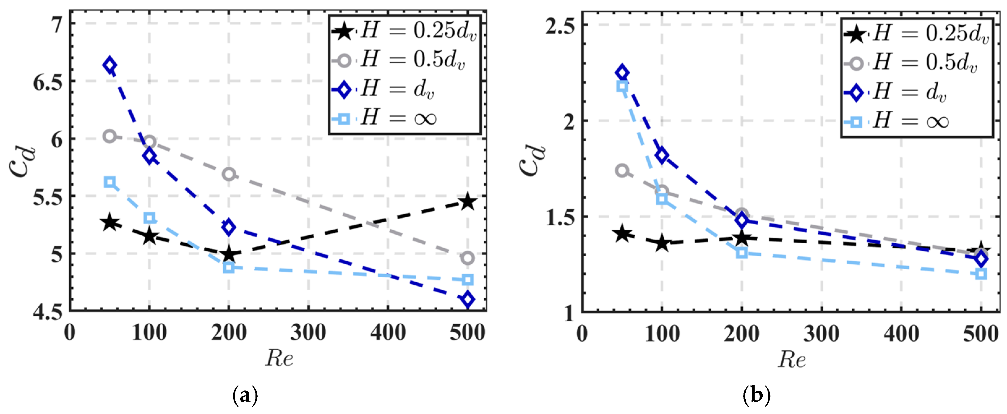
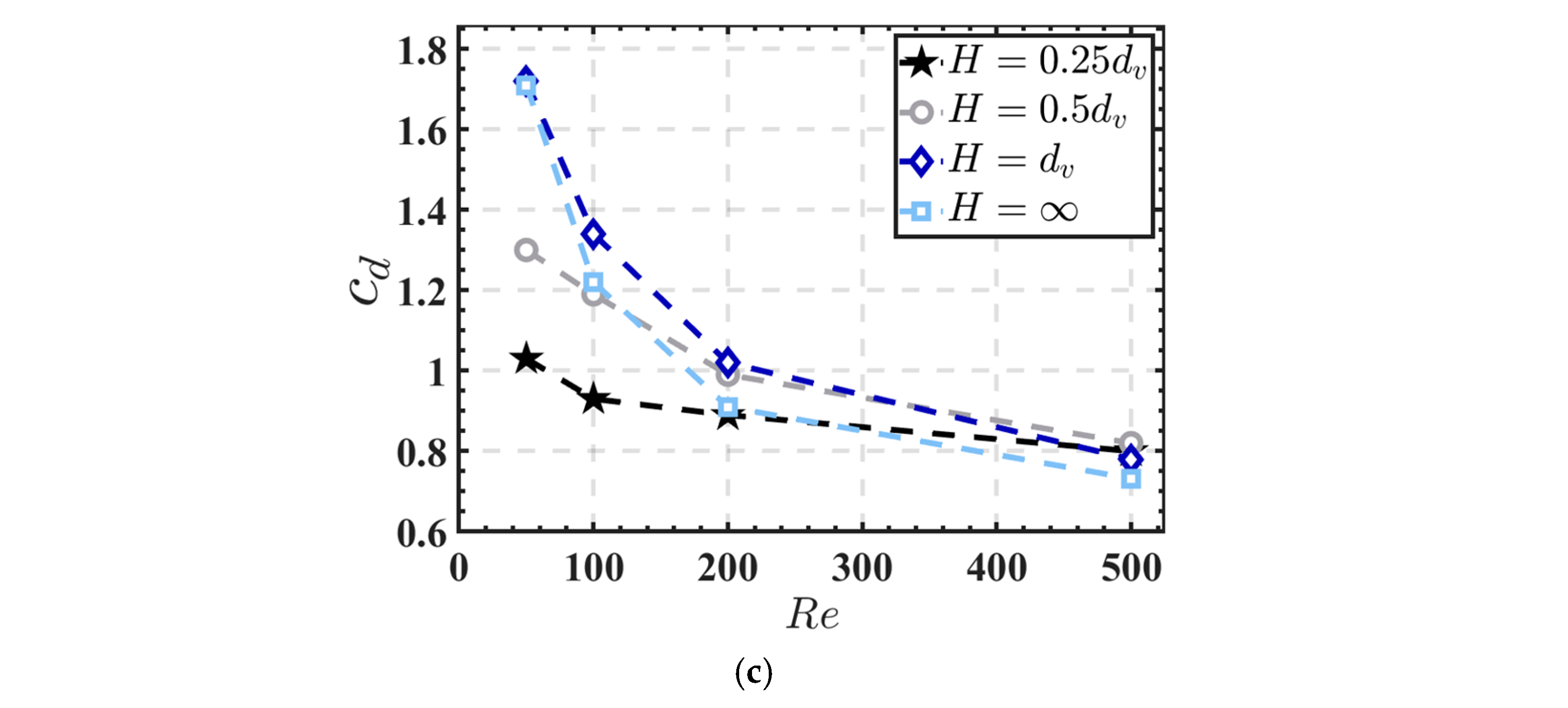
3.1. Influence of Reynolds Number on Drag Coefficient

The influence of particle–wall distance H on the drag coefficient of oblate spheroids was discussed in the previous section, and the rule of influence on the drag coefficient of particles near the wall will be discussed in this section. Figure 7 shows the flow diagram around the oblate spheroidal particles of $Ar$ = 0.5, $\theta =$0$°$, corresponding to$H$ = 0.25$d_v$, 0.5$d_v$, $d_v$, and$Re=$ 50, 500, respectively. As shown in Figure 7, at $Re=$ 50, when the particle is close to the wall ($H$= 0.25$d_v$), the blocking effect of the particle on the fluid is greater, the interstitial flow is weak, only a small amount of fluid flows under the particle, and the negative pressure generated behind the particle makes the fluid return to the back of the particle. As the particles gradually moved away from the wall, the interstitial flow gradually increased, the backflow behind the particles weakened, and a vortex formed at the bottom behind the particles (Figure 7c). When$Re$ = 500, the increase in fluid velocity makes the flow pattern more complex, and the fluid forms turbulent flow behind the particles when $H$= 0.25$d_v$, resulting in a chaotic flow state. With the increase in $H$, the flow pattern behind the particles becomes gradually stable and the streamline is gradually discernible (Figure 7f).

When the particles are near the wall $(Re$ = 50,$H$ = 0.5$d_v$), the fluid below the particles is strongly influenced by the wall. Under the joint action of the particles and the wall, the flow velocity increases, forming an interstitial flow similar to the jet stream and thus forming a stable vortex behind the particles. When $H$=$d_v$, the increase in the interstitial makes the interstitial flow stronger, thus increasing the size of the vortex. When Re is increased to 500 ($Re$= 500,$H$= 0.5$d_v$), the increase in fluid velocity causes the fluid to become unstable, the vortex is broken, and a chaotic turbulent flow is formed behind the particles. When the distance between the particle and walls is very small ($H$ = 0.25$d_v$), the velocity of the fluid with $Re$= 50 is very slow, and it still exists in the form of laminar flow behind the particles, and the flow lines behind the particles are clearly stratified. When the Reynolds number (Re) is 500, the fluid velocity increases, leading to a rise in the particle pressure differential drag force and the formation of a chaotic region downstream of the particle. But it can still be seen that two vortices of different sizes are formed behind the particle (Figure 7d).

Figure 8 shows the drag coefficient$c_d$ of oblate spheroids near the wall with different Reynolds numbers when $\theta$= 0°, corresponding to aspect ratio $Ar$ = 0.1, 0.5, and 0.8, respectively. It can be seen that the drag coefficient is largely dependent on the Reynolds number. For oblate spheroidal particles with an aspect ratio (Ar) of 0.1, the drag coefficient does not decrease monotonically as the Reynolds number (Re) increases when $H$= 0.25$d_v$. The drag coefficient ($c_d$) is higher at Re = 500 than at Re = 200 due to the larger windward area of the particles and the reduced particle–wall distance, which restricts fluid flow in the interstitial space and increases the differential drag force of the particle pressure. However, this hindrance effect is relatively weak at low velocity and has little effect on drag force. Therefore, when Reynolds number is small, the drag coefficient${ c}_d$still decreases with the increase in Reynolds number$Re$. For the oblate spheroidal particles with $Ar$= 0.5 and 0.8, its windward area is much smaller than that of the oblate ellipsoid with$Ar$= 0.1, and the obstructing effect of the same particles will be greatly weakened, so this change is not obvious (as shown in Figure 8b,c,$H$= 0.25$d_v$).

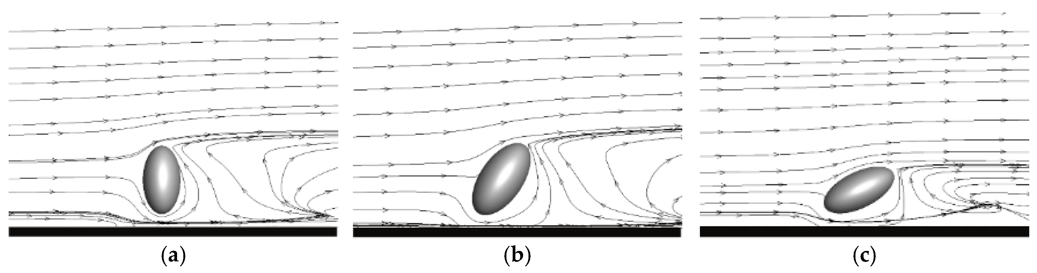
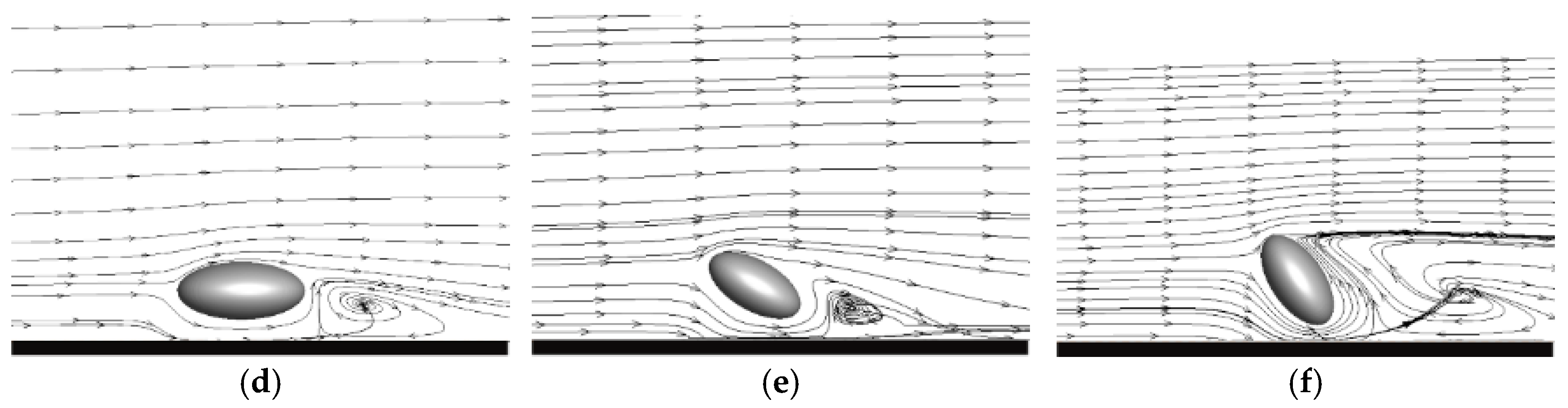
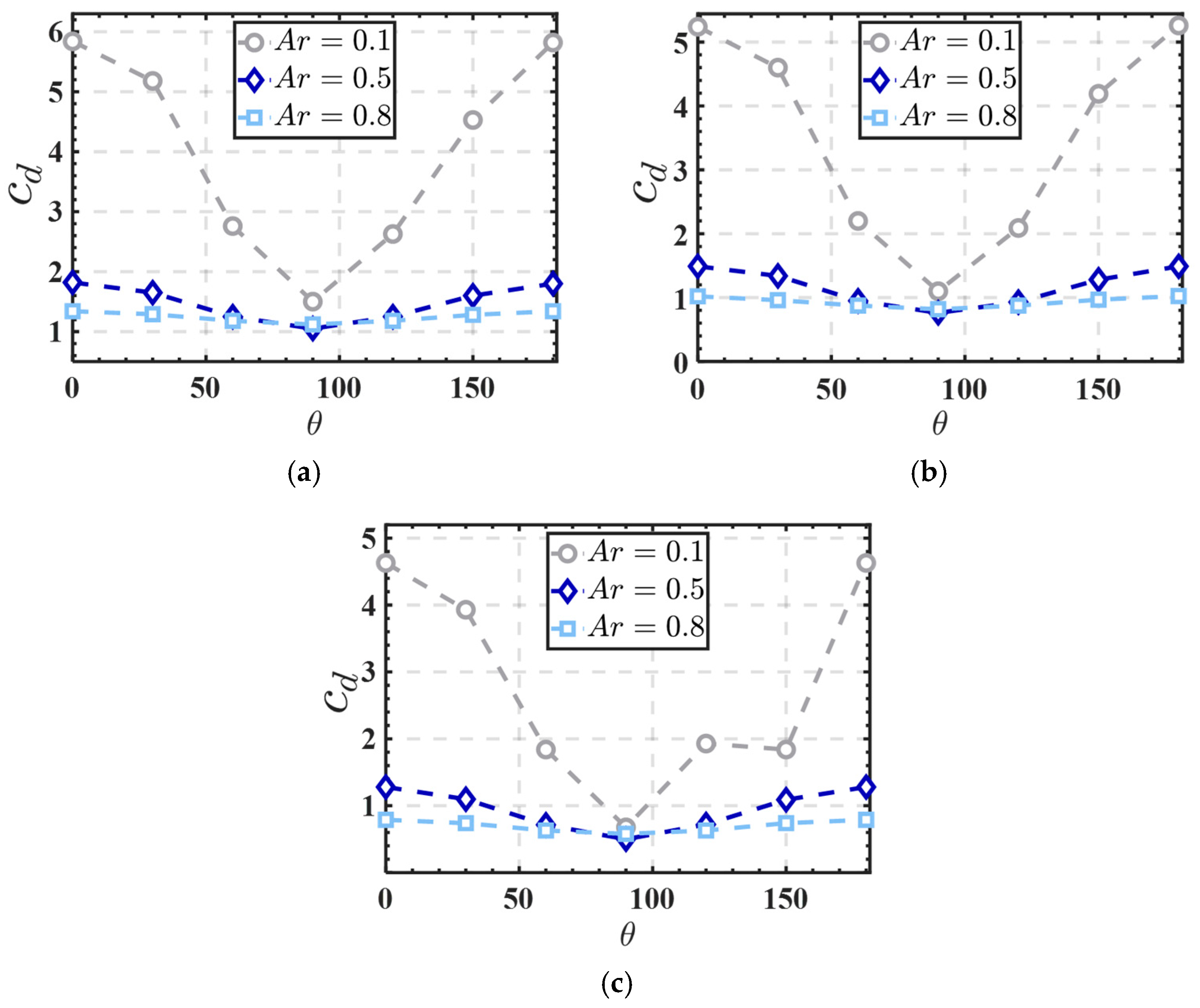
3.2. The Influence of Particle Orientation on the Drag Coefficient

Figure 9 shows the flow chart around the oblate spheroids with different particle orientations when$Ar$= 0.5, Re = 100, and$H$= 0.25$d_v$. It can be seen from Figure 9 that the particle orientation has a significant effect on the flow.

When$\theta =$ 0 (Figure 9a), the windward area of the particle is the largest, and a small vortex is formed farther behind the particle, because the negative pressure behind the particle causes the bottom fluid to form a reflux, and this part of the fluid meets the near-wall fluid to form a vortex. With the increase in particle orientation, when $\theta =$ 60$°$(Figure 9c), it is observed that the vortex gradually approaches the particle, and the front part of the particle is downward (the side that first contacts with the fluid is the front of the particle, that is, the left side of the particle). After experiencing a short narrow space, the fluid in the interstitial will gradually climb along the back of the oblate spheroids without converging with the vortex behind the particle. Therefore, the vortex can only maintain a small scale all the time. When $\theta =$ 90$°$(Figure 9d), the long axis of the ellipsoid particles is parallel to the flow direction, and the fluid in the interstitial will meet the reflux after passing through the interstitial to form a vortex, and the vortex size is increased compared with that at $\theta =$ 60$°$. When $\theta =$ 120$°$(Figure 9e), the front part of the particle faces upward, and a large amount of fluid enters the interstitial under the action of particle diversion, so the scale and intensity of the vortex behind the particle are enhanced. When $\theta =$ 150$°$, the front part of the particle continues to tilt upward. At this time, the effect of the particle on the incoming flow is greatly weakened, only a small part of the fluid enters the gap, and the vortex intensity weakens and only maintains a small scale.

3.3. The Effect of Aspect Ratio on the Drag Coefficient

The variation in drag coefficient $c_d$ for different aspect ratios is quantitatively shown in Figure 10. At $\theta$= 0°, the Ar = 0.1 oblate spheroidal particles has the largest obstruction effect on the fluid, and the drag coefficient $c_d$reaches the maximum at this time. With the increase in particle orientation, the windward area of particles decreases, and the drag coefficient $c_d$ also decreases. When $\theta$= 90°, the long axis of the particles is consistent with the direction of fluid flow, and the difference between the windward area of the three shapes of particles is very small at this time, and thus, the drag coefficient $c_d$ is also the closest.

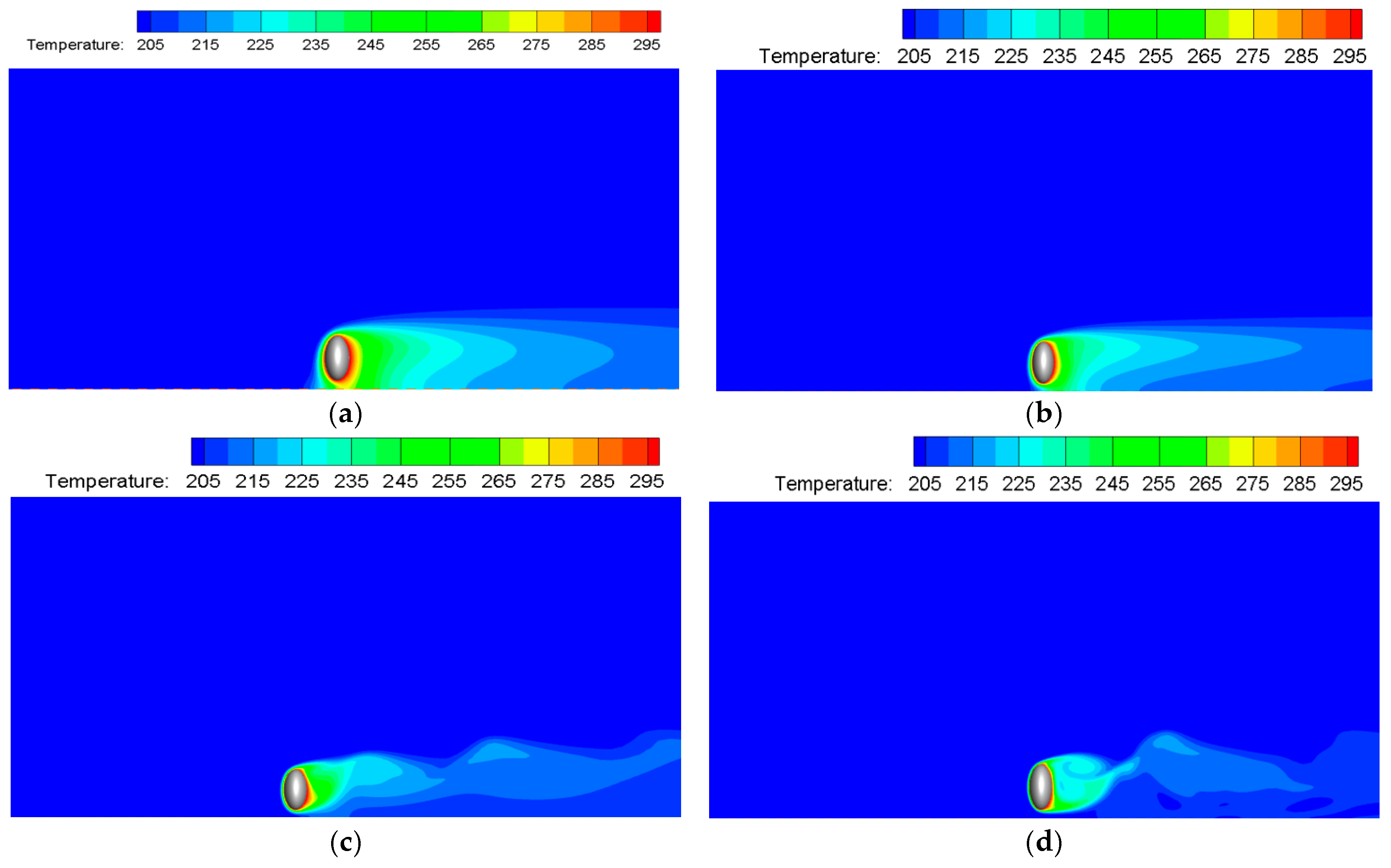
3.4. The Effect of Reynolds Number on Heat Transfer Performance

As shown in Figure 11, when the particle is close to the wall, the fluid below the particle is strongly influenced by the wall. When the Reynolds number is small (Figure 11a), the velocity of the fluid is slower, while the thickness of the boundary layer at the wall is larger, and a significant proportion of the fluid that completes the heat exchange with the particle adheres to the wall. When the Reynolds number increases to 100 (Figure 11b), the adhesion of the wall to the fluid weakens and the high-temperature fluid adhering to the wall is reduced. When the Reynolds number is increased to 200 (Figure 11c), a free jet is formed in the interstitial, and the high-temperature fluid is pushed away from the wall, at which time the interference of the wall to the particle heat transfer process basically disappears. Further, at Reynolds number$Re$= 500, a jet with high intensity has been formed in the interstitial, and the flow pattern of the high-temperature fluid tends to be disordered.

The Nusselt numbers$Nu$of oblate spheroidal particles with different Reynolds numbers are given in

Table 1. Nusselt numbers of particles with different Reynolds numbers ($Ar$= 0.5, $\theta$= 0$°$).

$\mathit{R}\mathit{e}$	$\mathit{N}{\mathit{u}}_{\mathit{u}}$	$\mathit{N}{\mathit{u}}_{0.25{\mathit{d}}_{\mathit{v}}}$	Deviation (%)
50	5.31	4.43	19.7
100	7.05	6.42	9.8
200	9.37	9.11	2.8
500	14.16	14.41	−1.7

to quantitatively discuss the effect of walls on the heat transfer performance of oblate spheroidal particles with different Reynolds numbers. In the table,$N{u}_u$denotes the particle Nusselt number in homogeneous flow, and$N{u}_{0.25d_v}$denotes the particle Nusselt number when$H$= 0.25$d_v$. The deviation is calculated using the formula $(N{u}_u-N{u}_{0.25d_v})/N{u}_{0.25d_v}$.

As shown in Table 1, the heat transfer capacity of the wall to the particles is reduced by nearly 20% when the Reynolds number is 50. With the increase in the Reynolds number, the interference of the wall to the heat transfer of the particles decreases rapidly, and when the Reynolds number is 200, the heat transfer of the particles is reduced by only 2%. This shows that the wall no longer hinders the heat transfer of particles.

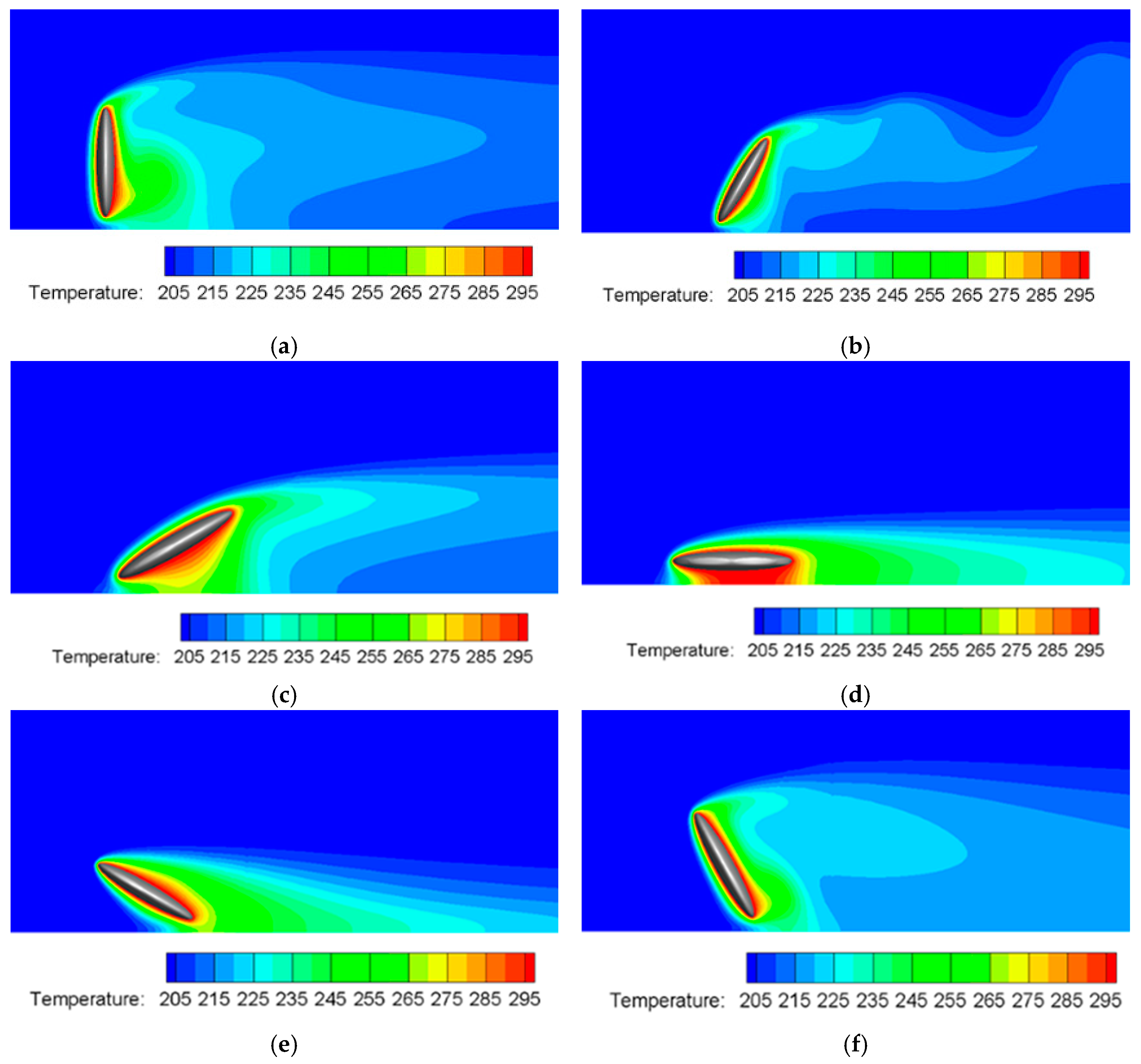
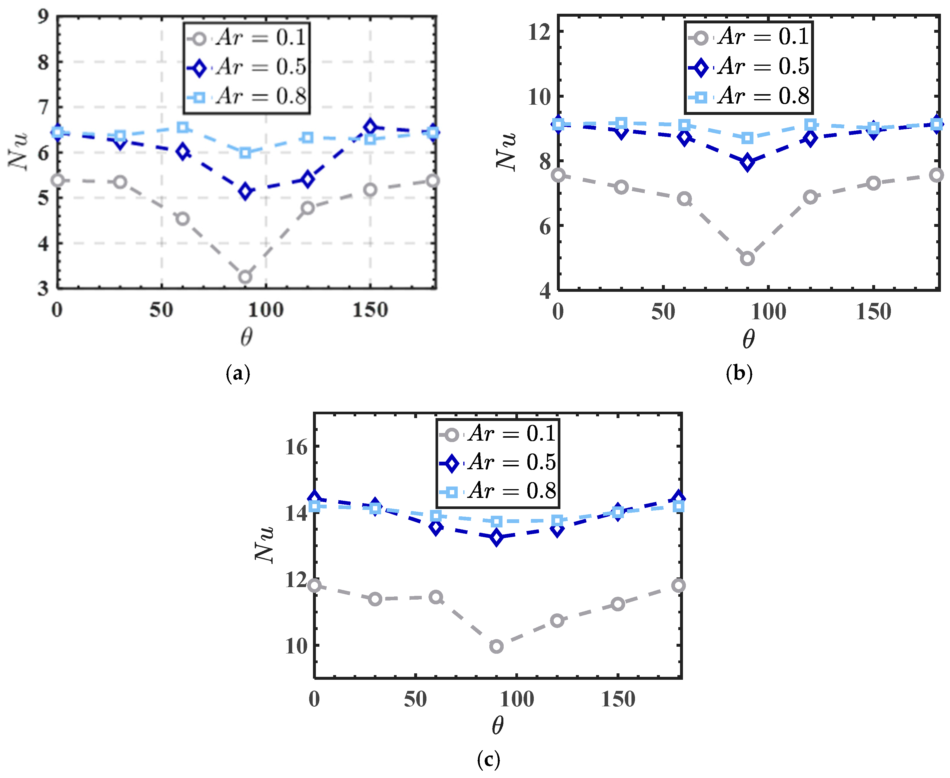
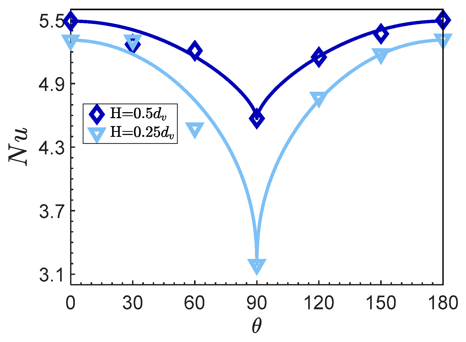
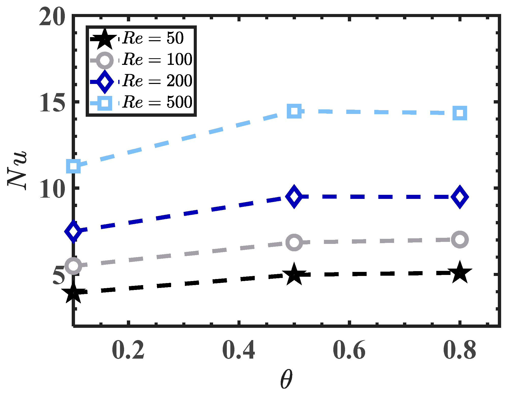
3.5. The Effect of Particle Orientation on Heat Transfer Performance

The heat transfer characteristics of oblate spheroids with different particle orientations near the wall are also quite different. The temperature cloud of the oblate spheroids with different particle orientations near the wall is given in Figure 12. When$\theta$ = 30$°$(Figure 12b), the angle between the long axis of the particles and the wall is larger, the interstitial between the particles and wall is short and gradually expanded, most of the fluid can transport heat away from the wall, and the temperature of the fluid adhering to the wall is lower and the quantity is small. As the particle orientation angle increases (Figure 12c), the particles incline to the wall, the particle–wall gap becomes narrower, and the proportion of fluid trapped on the wall in the gap increases. At$\theta$= 90$°$ (Figure 12d), the long axis of the particles is parallel to the wall, which makes the gap between the particle and the wall narrow and long. After entering the gap, a large amount of fluid adheres to the wall, and some of the fluid temperature is higher. At this time, the drag force of the wall to the heat transfer of particles is the greatest, and the heat transfer capacity of particles is the weakest. As the particle orientation angle continues to deflect upward (Figure 12e,f), the fluid adhering to the wall is reduced, and the heat transfer capacity of the particles is gradually enhanced.

Correspondingly, Figure 13 shows the Nusselt number $Nu$ of oblate spheroidal particles with different particle orientations. As shown, the wall seriously impedes the particle heat transfer when $\theta$ = 90$°$. At this time, the particle heat transfer capacity is also the weakest. But with the increase or decrease in the particle orientation, the blocking effect of the wall decreases, and the heat transfer capacity of the particles gradually recovers.

As shown in Figure 14, the following equation was fitted between the Nusselt number Nu and $\theta$ based on the numerical simulation results:

$$N{u}_{\theta }=N{u}_{{90}^{\circ }}+(N{u}_{0^{\circ }}-N{u}_{{90}^{\circ }})\left|{\cos }^m\theta \right|$$

(18)

The Nusselt number Nu reaches a maximum when $\theta$ = 0°, and Nu shows a change as $\theta$ changes from 0° to 90°, and reaches a minimum as $\theta$ becomes 90°. The solid lines represent the fit of the formula to the Nusselt number. And it can be found that the fit of the formula to the Nusselt number is good for different particle–wall distances.

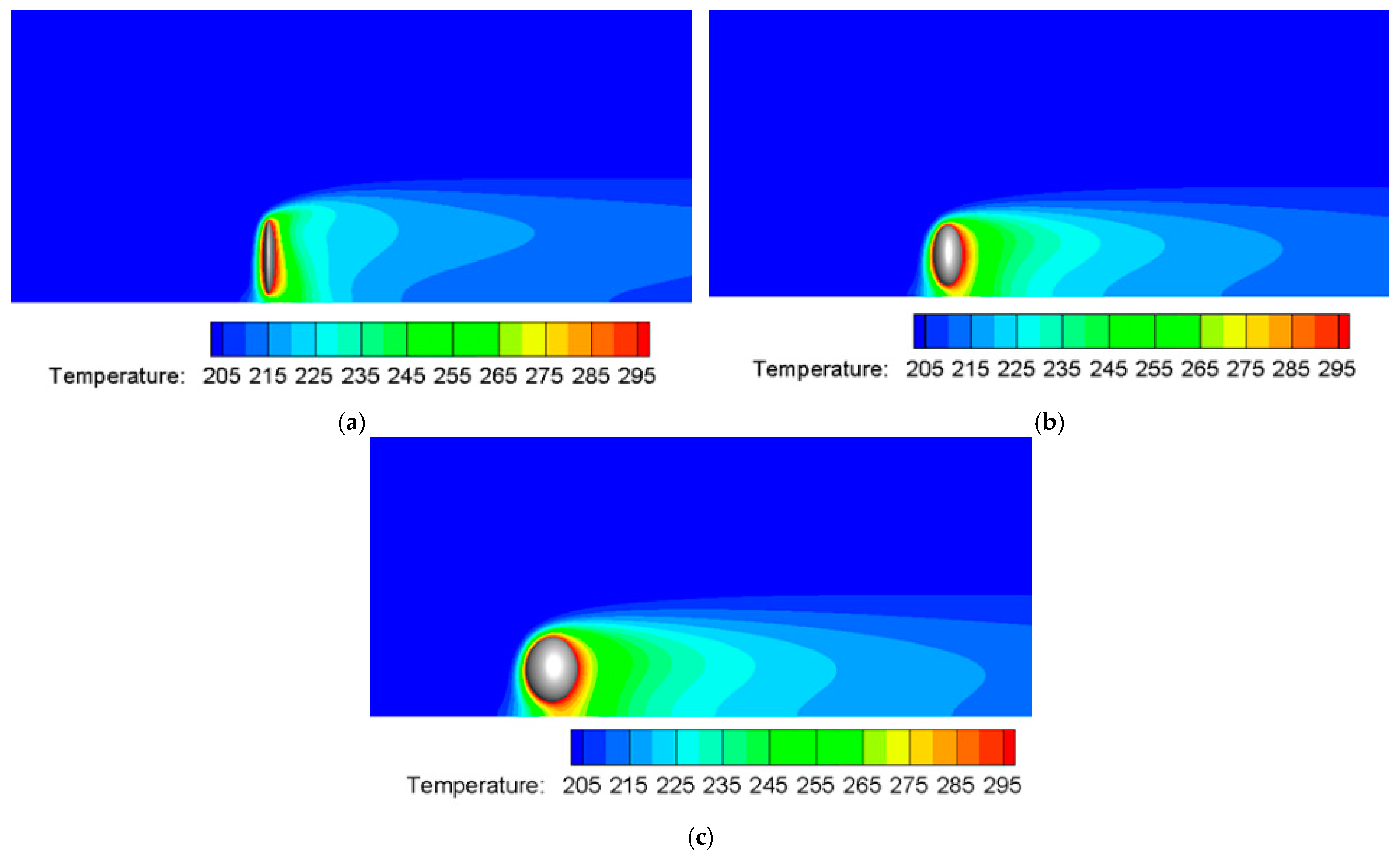
3.6. Effect of Aspect Ratio on the Heat Transfer Performance

Finally, the effect of the particle aspect ratio on heat transfer from oblate spheroids near the wall is discussed. As shown in Figure 15, the fluid temperature around the oblate spheroids with$Ar$= 0.1 is significantly lower than that of the oblate spheroids with$Ar$= 0.5 and$Ar$= 0.8, which is due to the larger windward area of the oblate spheroids with$Ar$= 0.1 and the smaller surface curvature of the particles, and the loss of kinetic energy of the fluid flowing through the surface of the particles is large, and the velocity of the fluid motion decreases rapidly. While the heat transfer between particles and fluid is mainly in the form of forced convection heat transfer, the decrease in fluid motion speed will lead to the weakening of forced convection heat transfer intensity and the decrease in heat transfer capacity. The oblate spheroid shape with$Ar$= 0.5 and$Ar$= 0.8 is closer to spherical shape, and the surface is smoother, and the fluid momentum loss through the surface of the particles is much smaller than the oblate spheroid with$Ar$= 0.1, so the heat transfer capacity is also stronger.

As shown in Figure 16, the heat transfer capacity of the particles increases with the increase in the particle aspect ratio$Ar$. And among these three shapes of particles, the oblate spheroid particles with$Ar$= 0.8 have the strongest heat transfer capacity.

4. Conclusions

This study explores the drag force and heat transfer characteristics of oblate spheroid particles in gas–solid two-phase flows near walls. In employing the Euler–Lagrangian model and large eddy simulation (LES), the effects of the Reynolds number, particle orientation, aspect ratio, and particle–wall distance on the drag coefficient and Nusselt number were systematically investigated. The key findings are as follows:

• Reynolds Number Influence: At Re = 500, turbulence mitigates wall interference, leading to a 14.4% increase in the Nusselt number (Nu) compared to lower Reynolds number cases. Simultaneously, wall-induced drag diminishes significantly, stabilizing the fluid flow.
• Particle Orientation Effect: When the particle’s long axis is parallel to the wall ($\theta$ = 90$°$), Nu decreases by 20%, indicating substantial flow obstruction. Conversely, orientations with a larger windward area result in a 35% increase in drag force compared to $\theta$ = 0°.
• Aspect Ratio Impact: Particles with higher aspect ratios (Ar = 0.8) demonstrate a 25% greater heat transfer efficiency and an 18% reduction in drag coefficient compared to those with Ar = 0.1, owing to enhanced aerodynamic properties and smoother flow interactions.
• Particle–Wall Distance Effect: As the particle–wall distance (H) increases from 0.25 to 0.5, wall-induced drag decreases by over 30%, reducing flow restrictions and enhancing heat transfer uniformity.

The findings contribute to the understanding of particle–fluid interactions in industrial applications such as pneumatic transport and crop drying, as well as natural phenomena. The optimized Euler–Lagrangian model offers a robust framework for simulating oblate spheroid particles, supporting advancements in computational fluid dynamics and practical engineering applications. Future studies could expand on the influence of particle roughness and irregularities to better represent real-world conditions.

References

1. Gray, J.M.N.T.; Gajjar, P.; Kokelaar, P. Particle-Size Segregation in Dense Granular Avalanches. C. R. Phys. 2015, 16, 73–85. [Google Scholar] [CrossRef]
2. Bao, X.; Wu, H.; Xiong, H.; Chen, X. Particle Shape Effects on Submarine Landslides via CFD-DEM. Ocean Eng. 2023, 284, 115140. [Google Scholar] [CrossRef]
3. Leonardi, A.; Wittel, F.K.; Mendoza, M.; Vetter, R.; Herrmann, H.J. Particle–Fluid–Structure Interaction for Debris Flow Impact on Flexible Barriers. Comput.-Aided Civ. Infrastruct. Eng. 2016, 31, 323–333. [Google Scholar] [CrossRef]
4. Chen, Q.; Xiong, T.; Zhang, X.; Jiang, P. Study of the Hydraulic Transport of Non-Spherical Particles in a Pipeline Based on the CFD-DEM. Eng. Appl. Comput. Fluid Mech. 2020, 14, 53–69. [Google Scholar] [CrossRef]
5. Tatemoto, Y.; Mibu, T.; Yokoi, Y.; Hagimoto, A. Effect of Freezing Pretreatment on the Drying Characteristics and Volume Change of Carrots Immersed in a Fluidized Bed of Inert Particles under Reduced Pressure. J. Food Eng. 2016, 173, 150–157. [Google Scholar] [CrossRef]
6. Zhong, W.; Yu, A.; Zhou, G.; Xie, J.; Zhang, H. CFD Simulation of Dense Particulate Reaction System: Approaches, Recent Advances and Applications. Chem. Eng. Sci. 2016, 140, 16–43. [Google Scholar] [CrossRef]
7. Kishore, N.; Gu, S. Momentum and Heat Transfer Phenomena of Spheroid Particles at Moderate Reynolds and Prandtl Numbers. Int. J. Heat Mass Transf. 2011, 54, 2595–2601. [Google Scholar] [CrossRef]
8. Motlagh, A.H.A.; Hashemabadi, S.H. 3D CFD Simulation and Experimental Validation of Particle-to-Fluid Heat Transfer in a Randomly Packed Bed of Cylindrical Particles. Int. Commun. Heat Mass Transf. 2008, 35, 1183–1189. [Google Scholar] [CrossRef]
9. Adamczyk, W.P.; Klimanek, A.; Białecki, R.A.; Węcel, G.; Kozołub, P.; Czakiert, T. Comparison of the Standard Euler–Euler and Hybrid Euler–Lagrange Approaches for Modeling Particle Transport in a Pilot-Scale Circulating Fluidized Bed. Particuology 2014, 15, 129–137. [Google Scholar] [CrossRef]
10. Zhang, Y.; Lu, X.-B.; Zhang, X.-H. An Optimized Eulerian–Lagrangian Method for Two-Phase Flow with Coarse Particles: Implementation in Open-Source Field Operation and Manipulation, Verification, and Validation. Phys. Fluids 2021, 33, 113307. [Google Scholar] [CrossRef]
11. Lyu, H.; Lucas, D.; Rzehak, R.; Schlegel, F. A Particle-Center-Averaged Euler-Euler Model for Monodisperse Bubbly Flows. Chem. Eng. Sci. 2022, 260, 117943. [Google Scholar] [CrossRef]
12. Zhao, Y.; Lu, B.; Zhong, Y. Euler–Euler Modeling of a Gas–Solid Bubbling Fluidized Bed with Kinetic Theory of Rough Particles. Chem. Eng. Sci. 2013, 104, 767–779. [Google Scholar] [CrossRef]
13. Frank, T. Parallele Algorithmen für Die Numerische Simulation Dreidimensionaler, Disperser Mehrphasenströmungen und Deren Anwendung in der Verfahrenstechnik; Shaker Verlag GmbH: Düren, Germany, 2002. [Google Scholar]
14. Ray, M.; Chowdhury, F.; Sowinski, A.; Mehrani, P.; Passalacqua, A. An Euler-Euler Model for Mono-Dispersed Gas-Particle Flows Incorporating Electrostatic Charging Due to Particle-Wall and Particle-Particle Collisions. Chem. Eng. Sci. 2019, 197, 327–344. [Google Scholar] [CrossRef]
15. Wittig, K.; Nikrityuk, P.; Richter, A. Drag Coefficient and Nusselt Number for Porous Particles under Laminar Flow Conditions. Int. J. Heat Mass Transf. 2017, 112, 1005–1016. [Google Scholar] [CrossRef]
16. Muyshondt, R.; Nguyen, T.; Hassan, Y.A.; Anand, N.K. Experimental Measurements of the Wake of a Sphere at Subcritical Reynolds Numbers. J. Fluids Eng. 2021, 143, 061301. [Google Scholar] [CrossRef]
17. Deen, N.G.; Kriebitzsch, S.H.L.; Van Der Hoef, M.A.; Kuipers, J.A.M. Direct Numerical Simulation of Flow and Heat Transfer in Dense Fluid–Particle Systems. Chem. Eng. Sci. 2012, 81, 329–344. [Google Scholar] [CrossRef]
18. Brian, P.L.T.; Hales, H.B. Effects of Transpiration and Changing Diameter on Heat and Mass Transfer to Spheres. AIChE J. 1969, 15, 419–425. [Google Scholar] [CrossRef]
19. Augier, F.; Idoux, F.; Delenne, J.Y. Numerical Simulations of Transfer and Transport Properties inside Packed Beds of Spherical Particles. Chem. Eng. Sci. 2010, 65, 1055–1064. [Google Scholar] [CrossRef]
20. Clift, R.; Grace, J.R.; Weber, M.E. Bubbles, Drops, and Particles; Courier Corporation: North Chelmsford, MA, USA, 2005. [Google Scholar]
21. Latham, J.-P.; Munjiza, A. The Modelling of Particle Systems with Real Shapes. Philos. Trans. R. Soc. Lond. Ser. A Math. Phys. Eng. Sci. 2004, 362, 1953–1972. [Google Scholar] [CrossRef]
22. Barker, D.A.; Arceo-Gomez, G. Pollen Transport Networks Reveal Highly Diverse and Temporally Stable Plant–Pollinator Interactions in an Appalachian Floral Community. AoB Plants 2021, 13, plab062. [Google Scholar] [CrossRef]
23. Chu, Y.-M.; Khan, U.; Shafiq, A.; Zaib, A. Numerical Simulations of Time-Dependent Micro-Rotation Blood Flow Induced by a Curved Moving Surface Through Conduction of Gold Particles with Non-Uniform Heat Sink/Source. Arab. J. Sci. Eng. 2021, 46, 2413–2427. [Google Scholar] [CrossRef]
24. Luo, S.; Feng, Y.; Song, J.; Xu, D.; Xia, K. Powder Fuel Transport Process and Mixing Characteristics in Cavity-Based Supersonic Combustor with Different Injection Schemes. Aerosp. Sci. Technol. 2022, 128, 107798. [Google Scholar] [CrossRef]
25. Zhong, W.; Yu, A.; Liu, X.; Tong, Z.; Zhang, H. DEM/CFD-DEM Modelling of Non-Spherical Particulate Systems: Theoretical Developments and Applications. Powder Technol. 2016, 302, 108–152. [Google Scholar] [CrossRef]
26. Roos, F.W.; Willmarth, W.W. Some Experimental Results on Sphere and Disk Drag. AIAA J. 1971, 9, 285–291. [Google Scholar] [CrossRef]
27. Yang, W.J.; Zhou, Z.Y.; Yu, A.B. Particle Scale Studies of Heat Transfer in a Moving Bed. Powder Technol. 2015, 281, 99–111. [Google Scholar] [CrossRef]
28. Yasuji, T.; Takeuchi, H.; Kawashima, Y. Particle Design of Poorly Water-Soluble Drug Substances Using Supercritical Fluid Technologies. Adv. Drug Deliv. Rev. 2008, 60, 388–398. [Google Scholar] [CrossRef] [PubMed]
29. Chen, Y.-L.; Qin, J.-C.; Sun, H.-P.; Shang, T.; Zhang, X.-G.; Hu, Y. Global Optimization for Cross-Domain Aircraft Based on Kriging Model and Particle Swarm Optimization Algorithm. Sci. Iran. 2021, 28, 209–222. [Google Scholar] [CrossRef]
30. Hottovy, J.D.; Sylvester, N.D. Drag Coefficients for Irregularly Shaped Particles. Ind. Eng. Chem. Proc. Des. Dev. 1979, 18, 433–436. [Google Scholar] [CrossRef]
31. Renganathan, K.; Turton, R.; Clark, N.N. Accelerating Motion of Geometric and Spherical Particles in a Fluid. Powder Technol. 1989, 58, 279–284. [Google Scholar] [CrossRef]
32. Kasper, G.; Niida, T.; Yang, M. Measurements of Viscous Drag on Cylinders and Chains of Spheres with Aspect Ratios between 2 and 50. J. Aerosol Sci. 1985, 16, 535–556. [Google Scholar] [CrossRef]
33. Wang, J.; Qi, H.; Zhu, J. Experimental Study of Settling and Drag on Cuboids with Square Base. Particuology 2011, 9, 298–305. [Google Scholar] [CrossRef]
34. Zhou, C.; Su, J.; Chen, H.; Shi, Z. Terminal Velocity and Drag Coefficient Models for Disc-Shaped Particles Based on the Imaging Experiment. Powder Technol. 2022, 398, 117062. [Google Scholar] [CrossRef]
35. Cebeci, T.; Meier, H. Turbulent Boundary Layers on a Prolate Spheroid. In Proceedings of the 19th AIAA, Fluid Dynamics, Plasma Dynamics, and Lasers Conference, Honolulu, HI, USA, 8–10 June 1987; American Institute of Aeronautics and Astronautics: Honolulu, HI, USA, 1987. [Google Scholar] [CrossRef]
36. Ganser, G.H. A Rational Approach to Drag Prediction of Spherical and Nonspherical Particles. Powder Technol. 1993, 77, 143–152. [Google Scholar] [CrossRef]
37. Haider, A.; Levenspiel, O. Drag Coefficient and Terminal Velocity of Spherical and Nonspherical Particles. Powder Technol. 1989, 58, 63–70. [Google Scholar] [CrossRef]
38. Hölzer, A.; Sommerfeld, M. New simple correlation formula for the drag coefficient of non-spherical particles. Powder Technol. 2008, 184, 361–365. [Google Scholar] [CrossRef]
39. Richter, A.; Nikrityuk, P.A. Drag Forces and Heat Transfer Coefficients for Spherical, Cuboidal and Ellipsoidal Particles in Cross Flow at Sub-Critical Reynolds Numbers. Int. J. Heat Mass Transf. 2012, 55, 1343–1354. [Google Scholar] [CrossRef]
40. Rong, L.W.; Zhou, Z.Y.; Yu, A.B. Lattice–Boltzmann Simulation of Fluid Flow through Packed Beds of Uniform Ellipsoids. Powder Technol. 2015, 285, 146–156. [Google Scholar] [CrossRef]
41. Sanjeevi, S.K.P.; Kuipers, J.A.M.; Padding, J.T. Drag, Lift and Torque Correlations for Non-Spherical Particles from Stokes Limit to High Reynolds Numbers. Int. J. Multiph. Flow 2018, 106, 325–337. [Google Scholar] [CrossRef]
42. Ke, C.; Shu, S.; Zhang, H.; Yuan, H.; Yang, D. On the Drag Coefficient and Averaged Nusselt Number of an Ellipsoidal Particle in a Fluid. Powder Technol. 2018, 325, 134–144. [Google Scholar] [CrossRef]
43. Mirhashemi, F.S.; Hashemabadi, S.H.; Noroozi, S. CFD Simulation and Experimental Validation for Wall Effects on Heat Transfer of Finite Cylindrical Catalyst. Int. Commun. Heat Mass Transf. 2011, 38, 1148–1155. [Google Scholar] [CrossRef]
44. El Hasadi, Y.M.F.; Padding, J.T. Solving fluid flow problems using semi-supervised symbolic regression on sparse data. AIP Adv. 2019, 9, 115218. [Google Scholar] [CrossRef]
45. Toghraie, D.; Afrand, M.; Zadeh, A.D.; Akbari, H.A. Numerical Investigation on the Flow and Heat Transfer of a Multi-Lobe Particle and Equivalent Spherical Particles in a Packed Bed with Considering the Wall Effects. Int. J. Mech. Sci. 2018, 138–139, 350–367. [Google Scholar] [CrossRef]
46. Zare, M.; Hashemabadi, S.H. Particle-Fluid Heat Transfer Close to the Bed Wall: CFD Simulation and Experimental Study of Particle Shape Influence on the Formation of Hot Zones. Int. J. Therm. Sci. 2020, 150, 106223. [Google Scholar] [CrossRef]
47. Pirozzoli, S.; Modesti, D.; Orlandi, P.; Grasso, F. Turbulence and Secondary Motions in Square Duct Flow. J. Fluid Mech. 2018, 840, 631–655. [Google Scholar] [CrossRef]
48. Yao, J.; Zhao, Y.; Fairweather, M. Numerical Simulation of Turbulent Flow through a Straight Square Duct. Appl. Therm. Eng. 2015, 91, 800–811. [Google Scholar] [CrossRef]
49. Zhang, H.; Trias, F.X.; Gorobets, A.; Tan, Y.; Oliva, A. Direct Numerical Simulation of a Fully Developed Turbulent Square Duct Flow up to Re τ = 1200. Int. J. Heat Fluid Flow 2015, 54, 258–267. [Google Scholar] [CrossRef]
50. Clark, R.A.; Ferziger, J.H.; Reynolds, W.C. Evaluation of Subgrid-Scale Models Using an Accurately Simulated Turbulent Flow. J. Fluid Mech. 1979, 91, 1–16. [Google Scholar] [CrossRef]
51. Ferziger, J.; Leslie, D. Large Eddy Simulation—A Predictive Approach to Turbulent Flow Computation. In Proceedings of the 4th Computational Fluid Dynamics Conference, Williamsburg, VA, USA, 23–25 July 1979; American Institute of Aeronautics and Astronautics: Williamsburg, VA, USA, 1979. [Google Scholar] [CrossRef]
52. Moin, P.; Kim, J. Numerical Investigation of Turbulent Channel Flow. J. Fluid Mech. 1982, 118, 341–377. [Google Scholar] [CrossRef]
53. Adams, J.F.W.; Fairweather, M.; Yao, J. Modelling and Simulation of Particle Re-Suspension in a Turbulent Square Duct Flow. Comput. Chem. Eng. 2011, 35, 893–900. [Google Scholar] [CrossRef]
54. Su, M.; Chen, Q.; Chiang, C.-M. Comparison of Different Subgrid-Scale Models of Large Eddy Simulation for Indoor Airflow Modeling. J. Fluids Eng. 2001, 123, 628–639. [Google Scholar] [CrossRef]
Figure 1. Definition of particle orientation of oblate spheroidal particle.
Water 17 00736 g001
Figure 2. Physical model setup of oblate ellipsoid near the wall.
Water 17 00736 g002
Figure 3. Grid division. (a) Overall grid diagram; (b) grid diagram around oblate spheroid.
Water 17 00736 g003
Figure 4. Calculation domain verification: Drag coefficient and Nusselt number verification ( θ   = 0 ° , A r   = 0.1, H   = 0.5 d v ). (a)   R e = 50 ;   (b) Re = 500.
Water 17 00736 g004
Figure 5. Influence of grid size on drag coefficient and Nusselt number ( θ   = 0 ° , A r   = 0.1, H   = 0.5 d v , Re = 500).
Water 17 00736 g005
Figure 6. The drag coefficient ( c d ) and Nusselt number (Nu) for prolate spheroids ( A r   = 2) under varying Reynolds numbers (Re) and particle orientations ( θ   = 0 ° , θ   = 90 ° ). (a) comparison of drag coefficient; (b) comparison of Nusselt number.
Water 17 00736 g006
Figure 7. Streamlines around oblate spheroids at different Re and H ( A r   = 0.25, θ   = 0 ° ). (a) H   = 0.25 d v ; (b) H   = 0.5 d v ; (c) H   =   d v ;   (d) H   = 0.25 d v ; (e) H   = 0.5 d v ; (f) H   =   d v .
Water 17 00736 g007
Figure 8. Drag coefficient ( c d ) for near-wall oblate spheroids with different Re values ( θ   = 0 ° ). (a)   A r   = 0.1; (b)   A r   = 0.5; (c)   A r   = 0.8.
Water 17 00736 g008aWater 17 00736 g008b
Figure 9. Oblate spheroid particle flow diagrams with different particle orientations ( A r   = 0.5, H   = 0.25 d v , R e   = 100). (a)   θ = 0 ° ; (b)   θ = 30 ° ; (c)   θ = 60 ° ;   (d)   θ = 90 ° ; (e)   θ = 120 ° ; (f)   θ = 15 0 ° .
Water 17 00736 g009aWater 17 00736 g009b
Figure 10. Drag coefficient   c d   of particles with different Ar values ( H   =   d v ). (a) Re = 100; (b) Re = 200; (c) Re = 500.
Water 17 00736 g010
Figure 11. Temperature clouds of particles with different Reynolds numbers   R e ( A r = 0.5,   H = 0.25 d v θ = 0 ° ). (a) Re = 50; (b) Re = 100; (c) Re = 200; (d) Re = 500.
Water 17 00736 g011
Figure 12. Temperature cloud map around an oblate spheroidal particle ( A r = 0.1,   R e = 100, H = 0.25 d v ). (a)   θ   = 0 ° ; (b)   θ   = 30 ° ; (c)   θ = 60 ° ; (d)   θ   = 90 ° ; (e)   θ   = 120 ° ; (f)   θ = 150 ° .
Water 17 00736 g012
Figure 13. Nusselt number N u of oblate spheroids with different particle orientations ( H = 0.25 d v ). (a) Re = 100; (b) Re = 200; (c) Re = 500.
Water 17 00736 g013
Figure 14. Fitting of Nusselt number Nu to particle orientation θ for different particle–wall distances (Re = 100).
Water 17 00736 g014
Figure 15. Temperature clouds of different Ar values of oblate spheroids near the wall surface ( R e   = 50, θ = 0 ° , H   = 0.25 d v ). (a)   A r   = 0.1; (b)   A r   = 0.5; (c)   A r   = 0.8.
Water 17 00736 g015
Figure 16. Nusselt number   N u   of different aspect ratios of oblate spheroids near the surface ( θ = 0 ° ,   H   = 0.5 d v ).
Water 17 00736 g016