
Hydraulic Characteristics of a New Vertical Slot Fishway with Staggered Baffles Configuration

Abstract
:1. Introduction
2. Materials and Methods
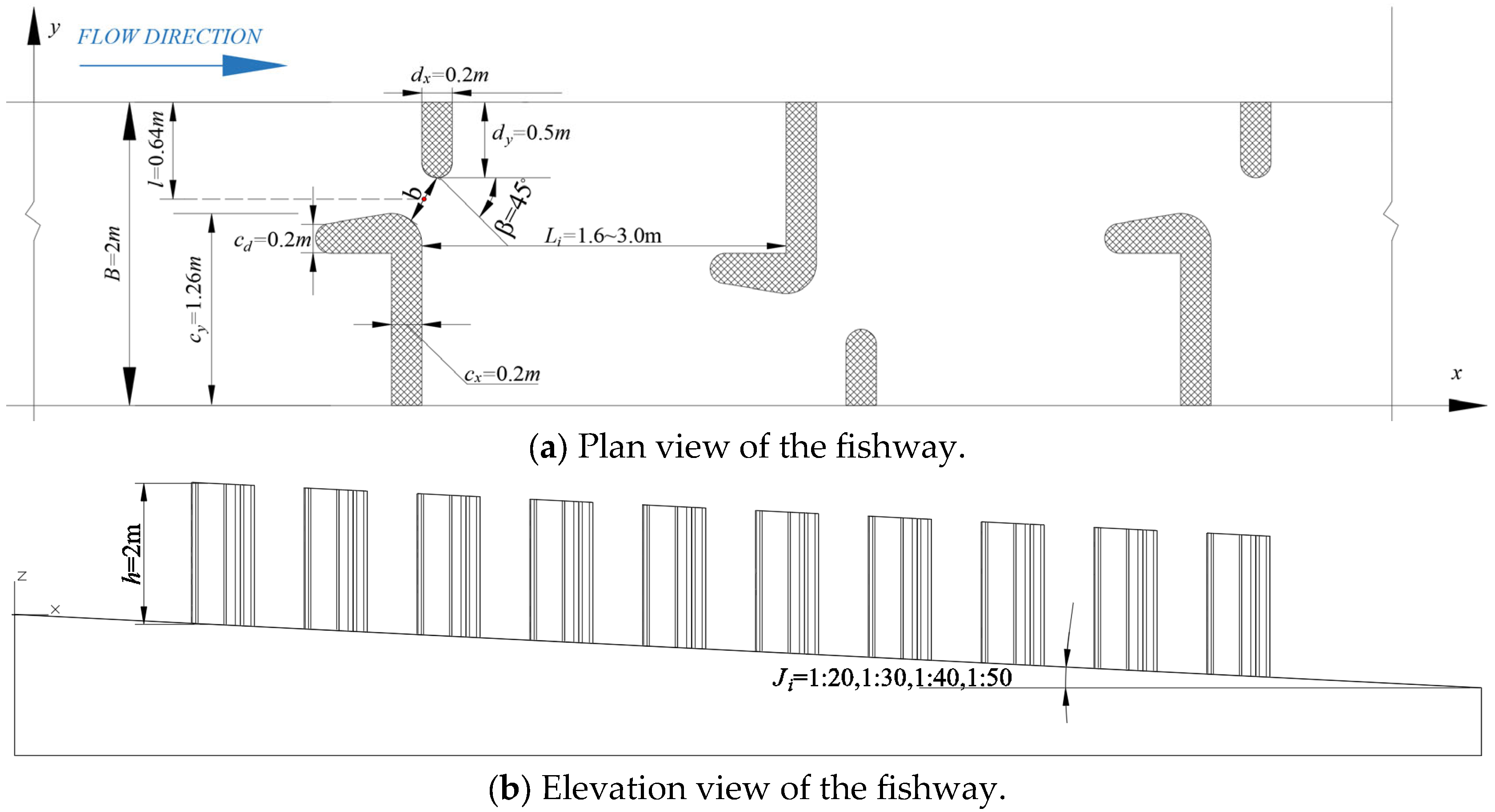
2.1. Research Object
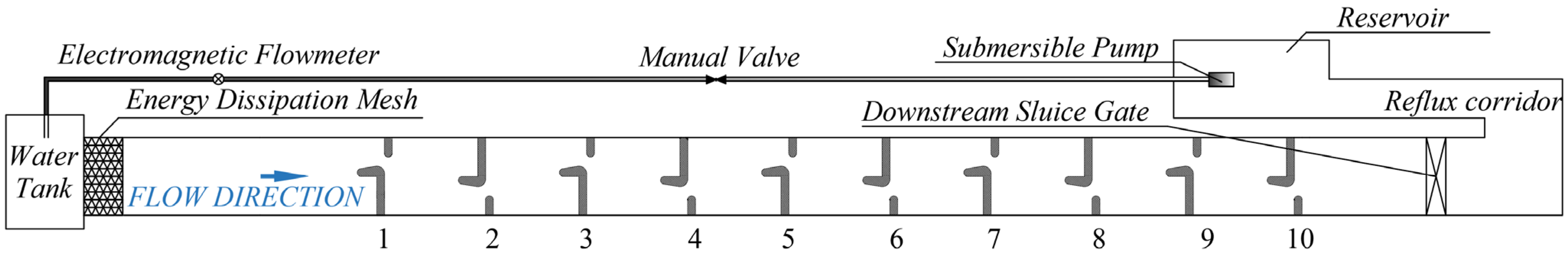
2.2. Physical Model
2.3. Numerical Simulation
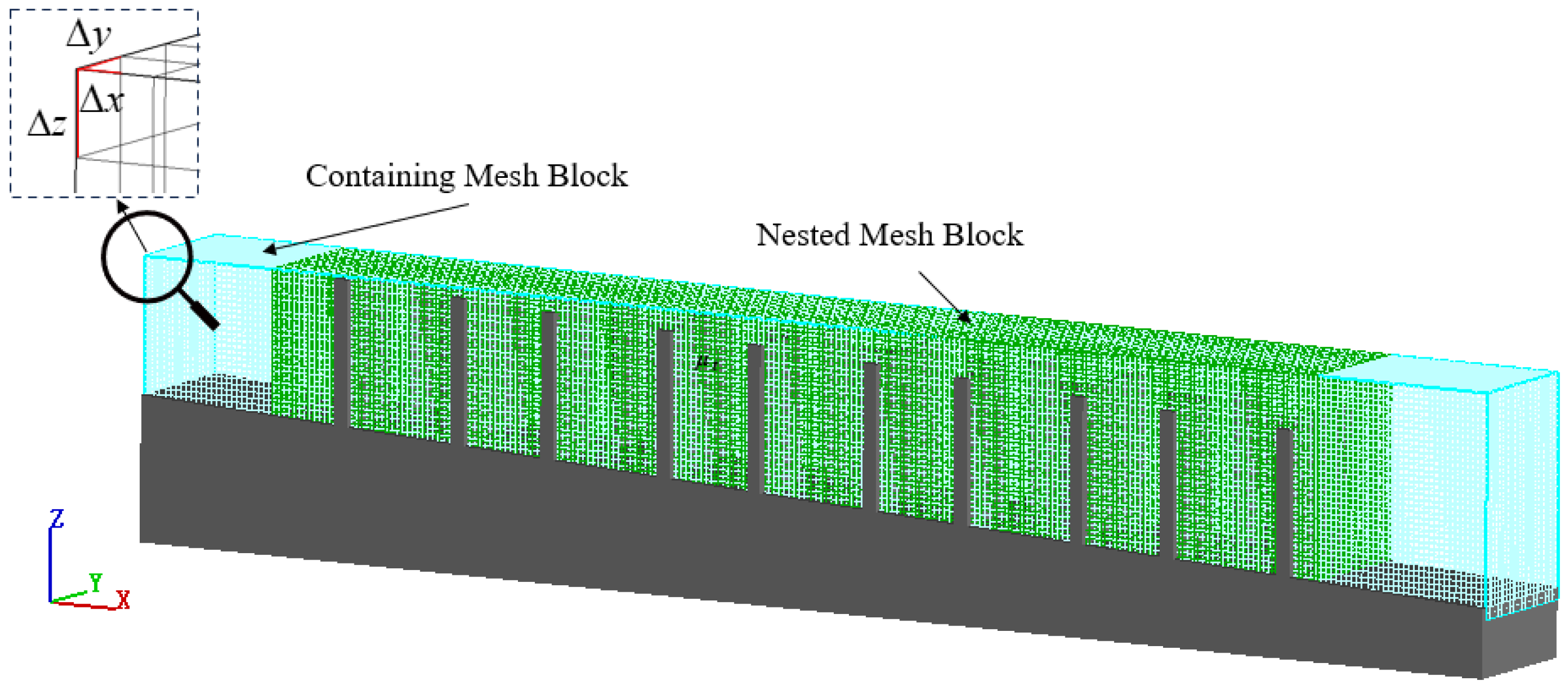
2.3.1. Model Establishment
2.3.2. Governing Equations
2.3.3. Turbulence Model
2.3.4. Boundary Conditions
2.4. Grid Independence Verification
3. Results and Discussion
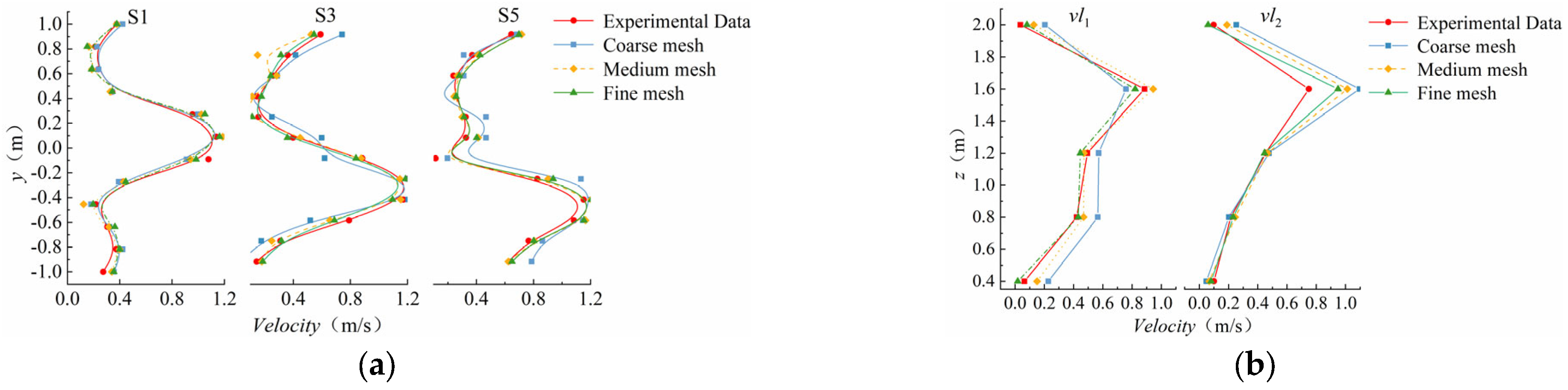
3.1. Model Validation
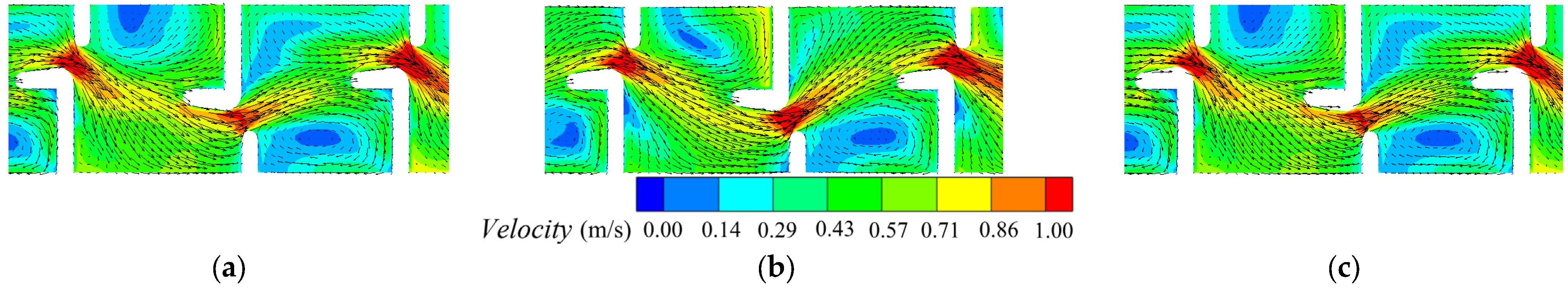
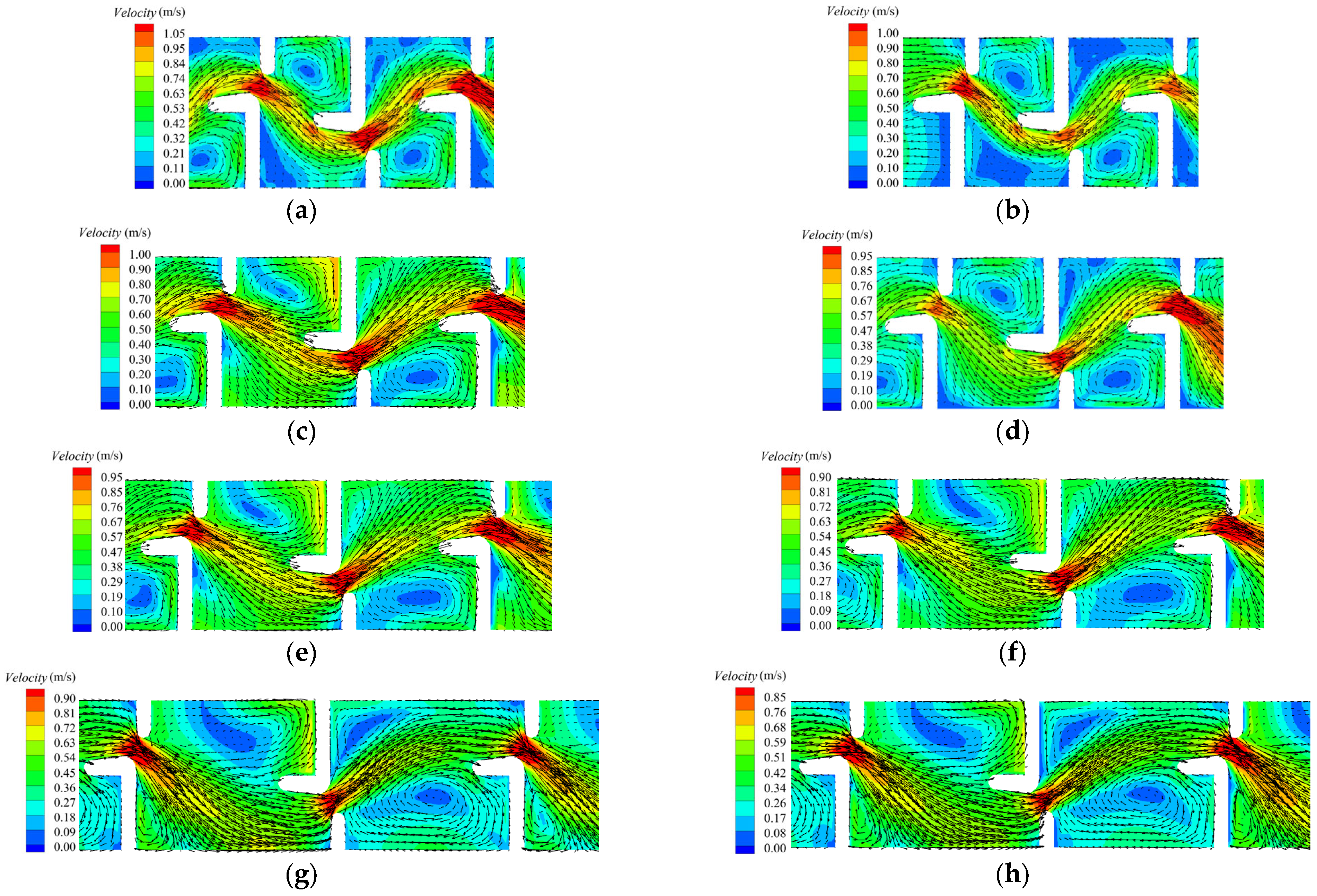
3.2. Flow Field
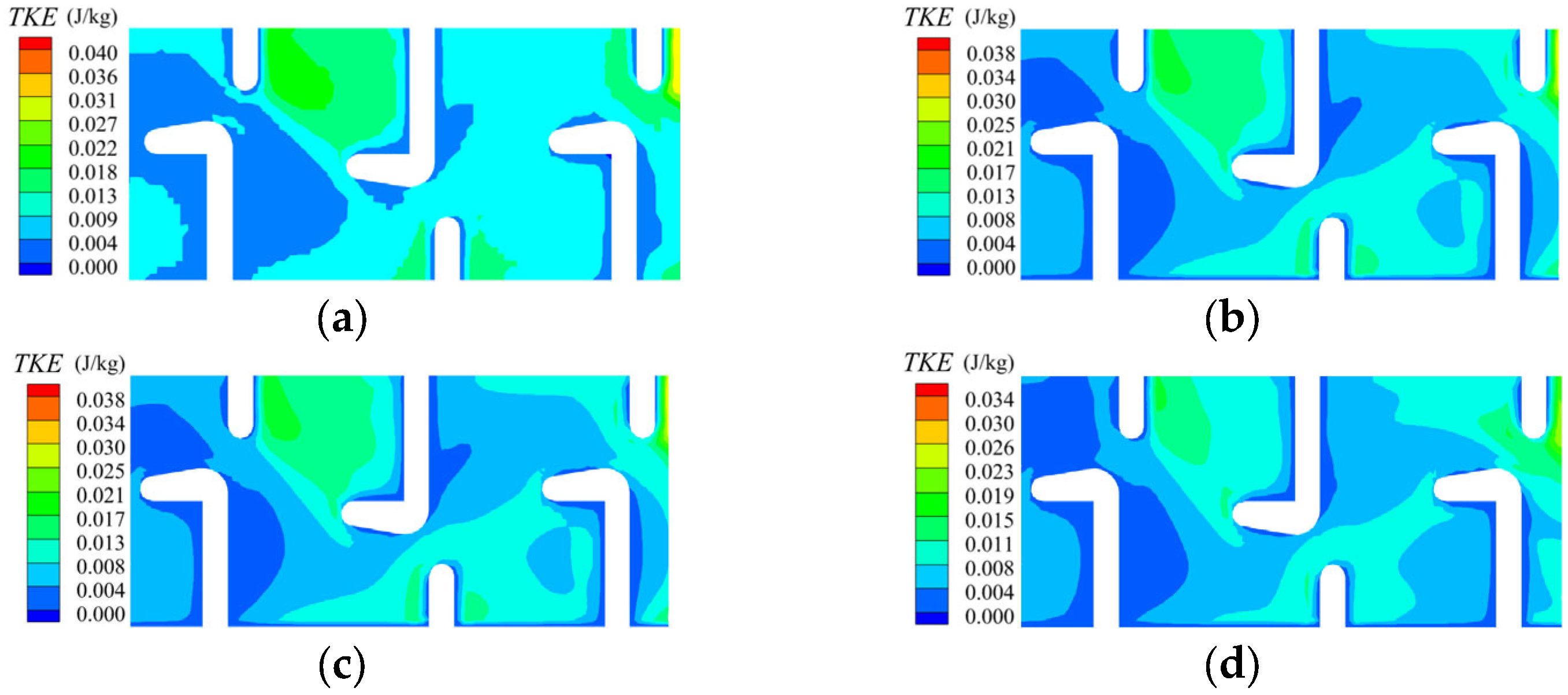
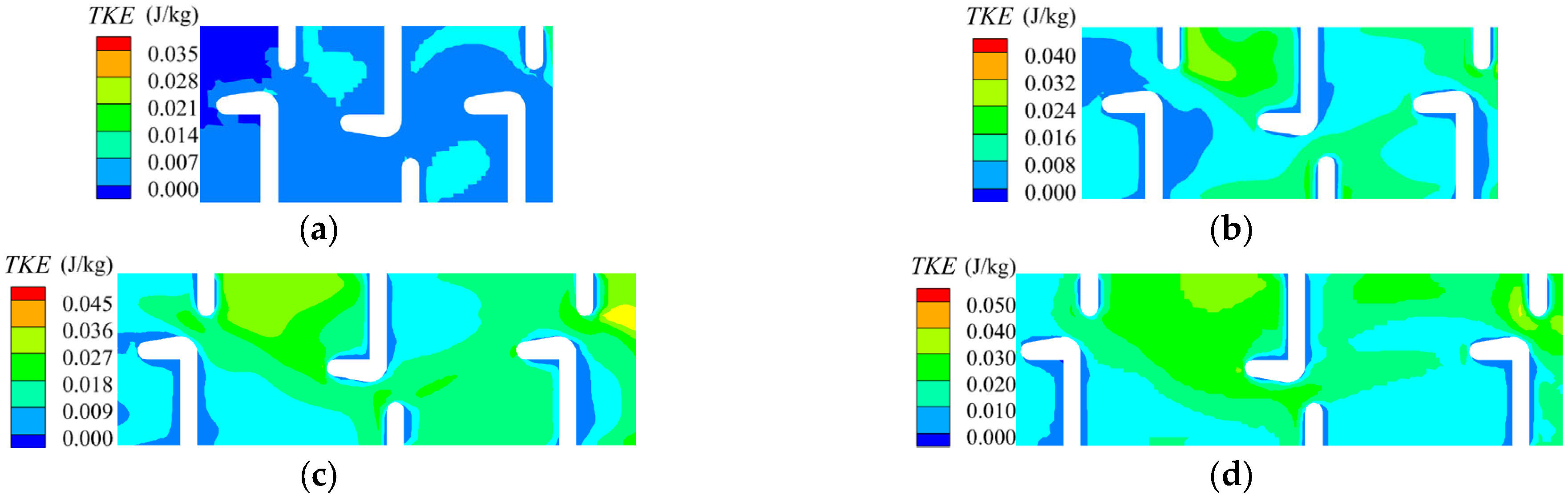
3.3. TKE
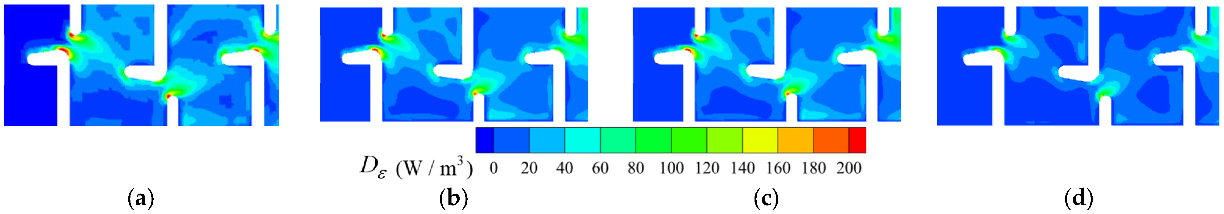
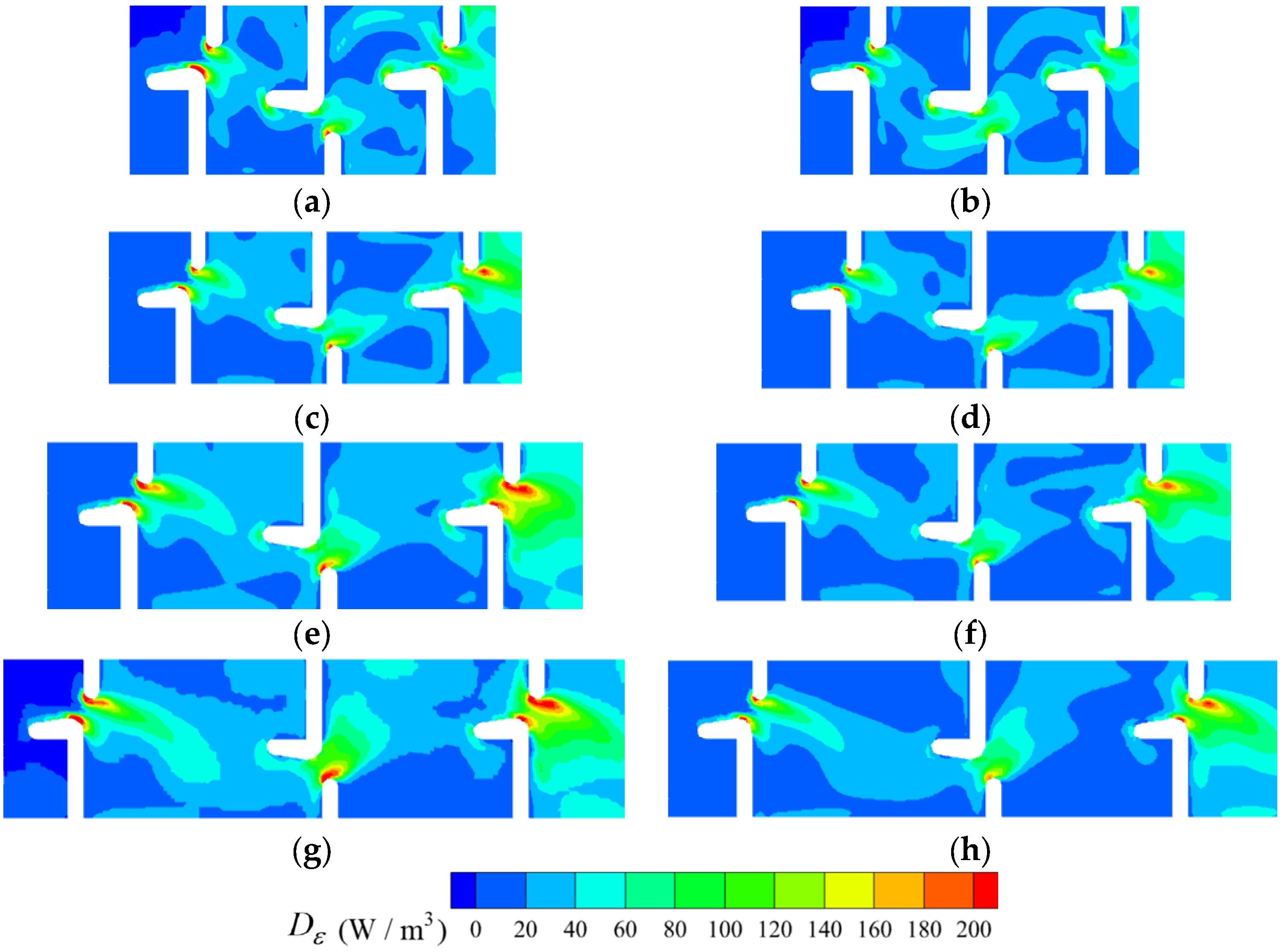
3.4. Volumetric Energy Dissipation
4. Conclusions
- (1)
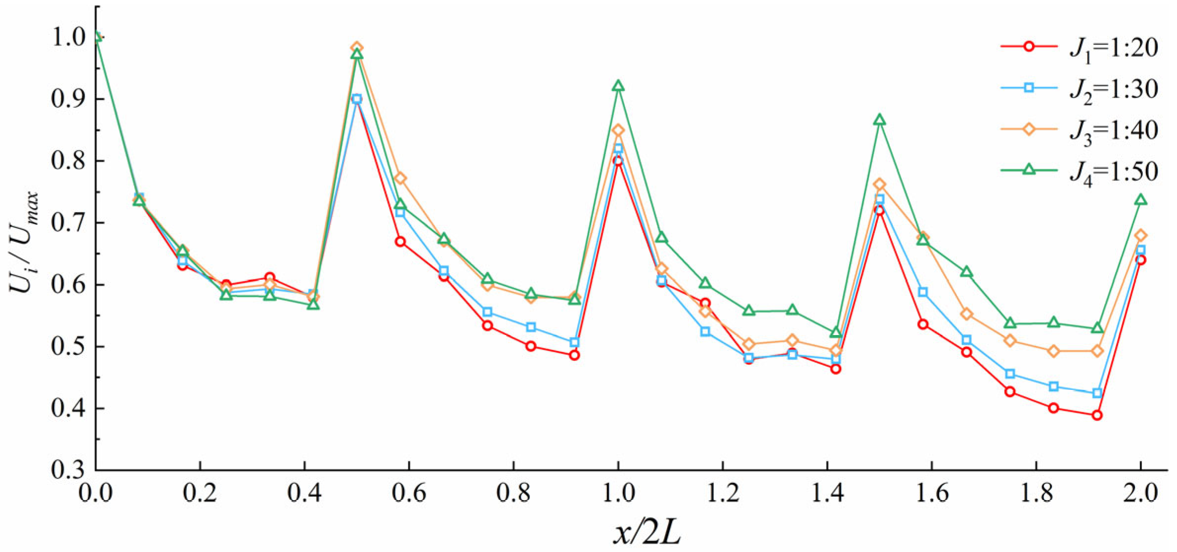
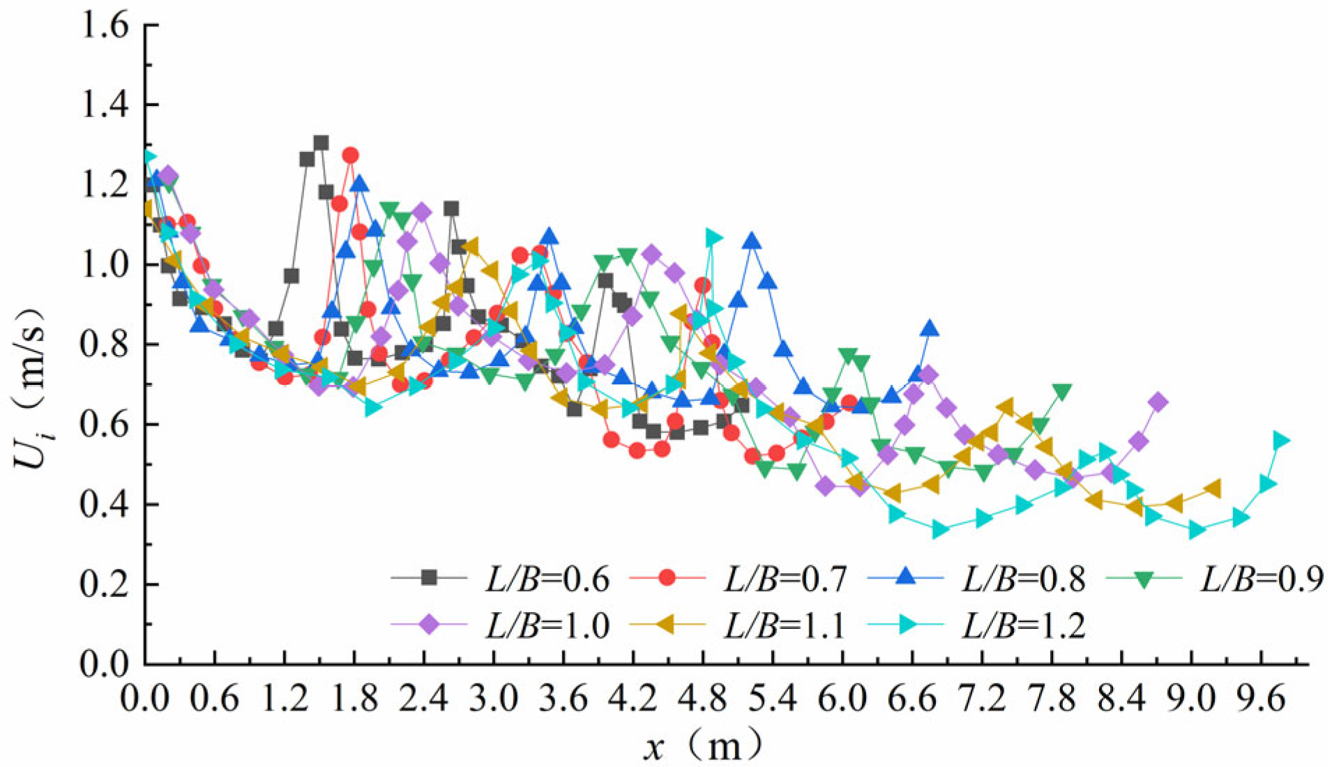
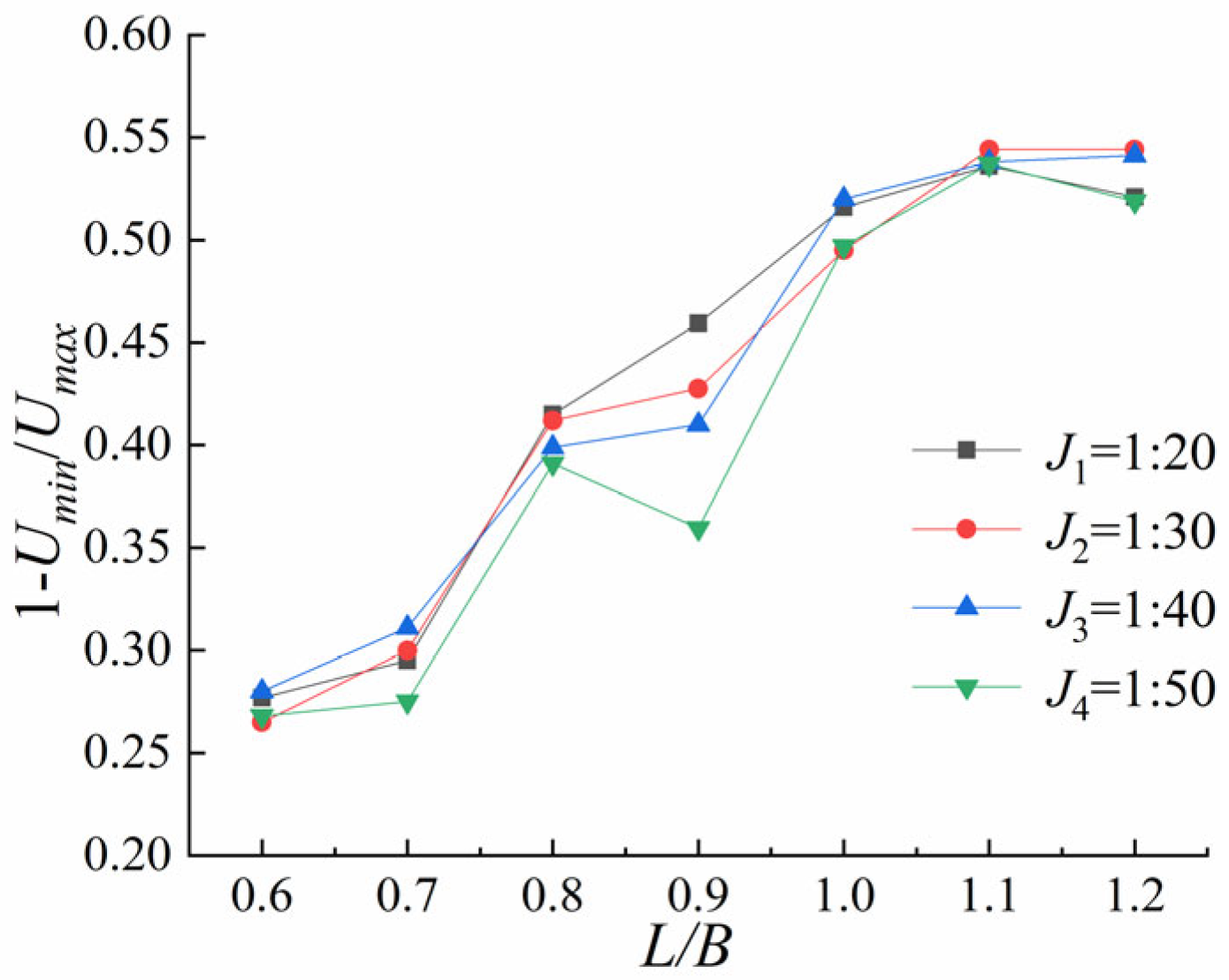
- Steeper slopes enhance the vertical-slot velocities and the chamber velocity differentials, thereby boosting the energy dissipation efficiency that is critical for fish migration. L/B ratios of 0.9–1.1 optimize the flow patterns, though increased slope steepness necessitates proportional adjustments to the L/B ratios.
- (2)
- Slope elevation amplifies the turbulent kinetic energy (TKE) at baffle junctions, whereas recirculation zones maintain stable turbulence levels, which are crucial for fish resting. When L/B exceeds or equals 1.2, TKE variations become predominantly governed by wall-attached flow.
- (3)
- Peak zones at baffle corners exhibit slope and L/B-dependent sensitivity; however, these regions are positioned outside the primary fish migration pathways, thus exerting minimal impact on upstream fish passage. The threshold of ≤ 150 W/m3—derived from fish endurance studies [58]—predominantly occurs in recirculation zones. Non-linear L/B relationships suggest optimal configurations that balance hydraulic performance with ecological requirements.
Author Contributions
Funding
Data Availability Statement
Acknowledgments
Conflicts of Interest
References
- Kuriqi, A.; Pinheiro, A.N.; Sordo-Ward, A.; Garrote, L. Influence of hydrologically based environmental flow methods on flow alteration and energy production in a run-of-river hydropower plant. J. Clean. Prod. 2019, 232, 1028–1042. [Google Scholar] [CrossRef]
- Chen, S.; Chen, B.; Fath, B.D. Assessing the cumulative environmental impact of hydropower construction on river systems based on energy network model. Renew. Sust. Energ. Rev. 2015, 42, 78–92. [Google Scholar] [CrossRef]
- Zarfl, C.; Berlekamp, J.; He, F.; Jähnig, S.C.; Darwall, W.; Tockner, K. Future large hydropower dams impact global freshwater megafauna. Sci. Rep. 2019, 9, 18531. [Google Scholar] [CrossRef] [PubMed]
- Couto, T.B.; Messager, M.L.; Olden, J.D. Safeguarding migratory fish via strategic planning of future small hydropower in Brazil. Nat. Sustain. 2021, 4, 409–416. [Google Scholar] [CrossRef]
- Verhelst, P.; Reubens, J.; Buysse, D.; Goethals, P.; Van Wichelen, J.; Moens, T. Toward a roadmap for diadromous fish conservation: The Big Five considerations. Front. Ecol. Environ. 2021, 19, 396–403. [Google Scholar] [CrossRef]
- Katopodis, C.; Cai, L.; Johnson, D. Sturgeon survival: The role of swimming performance and fish passage research. Fish. Res. 2019, 212, 162–171. [Google Scholar] [CrossRef]
- Quaranta, E.; Katopodis, C.; Comoglio, C. Effects of bed slope on the flow field of vertical slot fishways. River Res. Appl. 2019, 35, 656–668. [Google Scholar] [CrossRef]
- Ahmadi, M.; Ghaderi, A.; MohammadNezhad, H.; Kuriqi, A.; Di Francesco, S. Numerical investigation of hydraulics in a vertical slot fishway with upgraded configurations. Water 2021, 13, 2711. [Google Scholar] [CrossRef]
- An, R.; Li, J.; Liang, R.; Tuo, Y. Three-dimensional simulation and experimental study for optimising a vertical slot fishway. J. Hydro-Environ. Res. 2016, 12, 119–129. [Google Scholar] [CrossRef]
- Tarrade, L.; Texier, A.; David, L.; Larinier, M. Topologies and measurements of turbulent flow in vertical slot fishways. Hydrobiologia 2008, 609, 177–188. [Google Scholar] [CrossRef]
- Calluaud, D.; Pineau, G.; Texier, A.; David, L. Modification of vertical slot fishway flow with a supplementary cylinder. J. Hdraul. Res. 2014, 52, 614–629. [Google Scholar] [CrossRef]
- Sanagiotto, D.G.; Rossi, J.B.; Bravo, J.M. Applications of computational fluid dynamics in the design and rehabilitation of nonstandard vertical slot fishways. Water 2019, 11, 199. [Google Scholar] [CrossRef]
- Zhang, D.; Xu, Y.; Deng, J.; Shi, X.; Liu, Y. Relationships among the fish passage efficiency, fish swimming behavior, and hydraulic properties in a vertical-slot fishway. Fish. Manag. Ecol. 2024, 31, e12681. [Google Scholar] [CrossRef]
- Chorda, J.; Maubourguet, M.M.; Roux, H.; Larinier, M.; Tarrade, L.; David, L. Two-dimensional free surface flow numerical model for vertical slot fishways. J. Hydraul. Res. 2010, 48, 141–151. [Google Scholar] [CrossRef]
- Tarrade, L.; Pineau, G.; Calluaud, D.; Texier, A.; David, L.; Larinier, M. Detailed experimental study of hydrodynamic turbulent flows generated in vertical slot fishways. Environ. Fluid Mech. 2011, 11, 1–21. [Google Scholar] [CrossRef]
- Puertas, J.; Pena, L.; Teijeiro, T. Experimental approach to the hydraulics of vertical slot fishways. J. Hydraul. Eng. 2004, 130, 10–23. [Google Scholar] [CrossRef]
- Ahmadi, M.; Kuriqi, A.; Nezhad, H.M.; Ghaderi, A.; Mohammadi, M. Innovative configuration of vertical slot fishway to enhance fish swimming conditions. J. Hydrodyn. 2022, 34, 917–933. [Google Scholar] [CrossRef]
- Rajaratnam, N.; Katopodis, C.; Solanki, S. New designs for vertical slot fishways. Can. J. Civ. Eng. 1992, 19, 402–414. [Google Scholar] [CrossRef]
- Wang, R.W.; David, L.; Larinier, M. Contribution of experimental fluid mechanics to the design of vertical slot fish passes. Knowl. Manag. Aquat. Ecosyst. 2010, 396, 2. [Google Scholar] [CrossRef]
- Peake, S.J.; Beamish, F.W.; McKinley, R.S.; Scruton, D.A.; Katopodis, C. Relating swimming performance of lake sturgeon, Acipenser fulvescens, to fishway desing. Can. J. Fish Aquat. Sci. 1997, 54, 1361–1366. [Google Scholar] [CrossRef]
- Tan, J.; Li, H.; Guo, W.; Tan, H.; Ke, S.; Wang, J.; Shi, X. Swimming performance of four carps on the Yangtze River for fish passage design. Sustainability 2021, 13, 1575. [Google Scholar] [CrossRef]
- Li, H.; Cai, D.; Yang, P. Swimming ability and behavior of different sized silver carp. J. Hydroecol. 2016, 37, 88–92. [Google Scholar]
- Hou, Y.; Newbold, L.; Cai, L.; Wang, X.; Hu, W.; Qiao, Y. Swimming performance of juvenile Aristichthys nobilis under fixed velocity swimming tests. Chin. J. Ecol. 2016, 35, 1583–1588. [Google Scholar]
- Bombač, M.; Novak, G.; Rodič, P.; Četina, M. Numerical and physical model study of a vertical slot fishway. J. Hydrol. Hydromech. 2014, 62, 150–159. [Google Scholar] [CrossRef]
- Tarena, F.; Nyqvist, D.; Katopodis, C.; Comoglio, C. Computational fluid dynamics in fishway research-a systematic review on upstream fish passage solutions. J. Ecohydraul. 2024, 10, 107–126. [Google Scholar] [CrossRef]
- Fuentes-Pérez, J.F.; Quaresma, A.L.; Pinheiro, A.; Sanz-Ronda, F.J. OpenFOAM vs. FLOW-3D: A comparative study of vertical slot fishway modelling. Ecol. Eng. 2022, 174, 106446. [Google Scholar] [CrossRef]
- Flow Science, Inc. Flow-3D Version 11.2 User Manual; Flow Science, Inc.: Los Alamos, NM, USA, 2016. [Google Scholar]
- Dargahi, B. Flow characteristics of bottom outlets with moving gates. J. Hydraul. Res. 2010, 48, 476–482. [Google Scholar] [CrossRef]
- Savage, B.M.; Johnson, M.C. Flow over ogee spillway: Physical and numerical model case study. J. Hydraul. Eng. 2001, 127, 640–649. [Google Scholar] [CrossRef]
- Bombardelli, F.A.; Meireles, I.; Matos, J. Laboratory measurements and multi-block numerical simulations of the mean flow and turbulence in the non-aerated skimming flow region of steep stepped spillways. Environ. Fluid Mech. 2011, 11, 263–288. [Google Scholar] [CrossRef]
- Abad, J.D.; Rhoads, B.L.; Güneralp, İ.; Garcia, M.H. Flow structure at different stages in a meander-bend with bendway weirs. J. Hydraul. Eng. 2008, 134, 1052–1063. [Google Scholar] [CrossRef]
- Duguay, J.M.; Lacey, R.W.J.; Gaucher, J. A case study of a pool and weir fishway modeled with OpenFOAM and FLOW-3D. Ecol. Eng. 2017, 103, 31–42. [Google Scholar] [CrossRef]
- Bayon, A.; Valero, D.; García-Bartual, R.; López-Jiménez, P.A. Performance assessment of OpenFOAM and FLOW-3D in the numerical modeling of a low Reynolds number hydraulic jump. Environ. Model. Softw. 2016, 80, 322–335. [Google Scholar] [CrossRef]
- Hirt, C.W.; Nichols, B.D. Volume of fluid (VOF) method for the dynamics of free boundaries. J. Comput. Phys. 1981, 39, 201–225. [Google Scholar] [CrossRef]
- Ghaderi, A.; Abbasi, S. Experimental and numerical study of the effects of geometric appendance elements on energy dissipation over stepped spillway. Water 2021, 13, 957. [Google Scholar] [CrossRef]
- Daneshfaraz, R.; Ghaderi, A.; Sattariyan, M.; Alinejad, B.; Asl, M.M.; Di Francesco, S. Investigation of local scouring around hydrodynamic and circular pile groups under the influence of river material harvesting pits. Water 2021, 13, 2192. [Google Scholar] [CrossRef]
- Di Francesco, S.; Biscarini, C.; Manciola, P. Numerical simulation of water free-surface flows through a front-tracking lattice Boltzmann approach. J. Hydroinf. 2015, 17, 1–6. [Google Scholar] [CrossRef]
- Silva, A.T.; Bermúdez, M.; Santos, J.M.; Rabuñal, J.R.; Puertas, J. Pool-type fishway design for a potamodromous cyprinid in the Iberian Peninsula: The Iberian barbel—Synthesis and future directions. Sustainability 2020, 12, 3387. [Google Scholar] [CrossRef]
- Roache, P.J. Perspective: A method for uniform reporting of grid refinement studies. J. Fluids Eng. 1994, 116, 405–413. [Google Scholar] [CrossRef]
- Quaresma, A.L.; Romao, F.; Branco, P.; Ferreira, M.T.; Pinheiro, A.N. Multi slot versus single slot pool-type fishways: A modelling approach to compare hydrodynamics. Ecol. Eng. 2018, 122, 197–206. [Google Scholar] [CrossRef]
- Ghaderi, A.; Dasineh, M.; Aristodemo, F.; Aricò, C. Numerical simulations of the flow field of a submerged hydraulic jump over triangular macroroughnesses. Water 2021, 13, 674. [Google Scholar] [CrossRef]
- Pourshahbaz, H.; Abbasi, S.; Pandey, M.; Pu, J.H.; Taghvaei, P.; Tofangdar, N. Morphology and hydrodynamics numerical simulation around groynes. ISH J. Hydraul. Eng. 2022, 28, 53–61. [Google Scholar] [CrossRef]
- Yakhot, V.; Orszag, S.A. Renormalization group analysis of turbulence. I. Basic theory. J. Sci. Comput. 1986, 1, 3–51. [Google Scholar] [CrossRef]
- Santos, H.A.; Pinheiro, A.P.; Mendes, L.M.M.; Junho, R.A.C. Turbulent flow in a central vertical slot Fishway: Numerical assessment with RANS and LES schemes. J. Irrig. Drain. Eng. 2022, 148, 04022025. [Google Scholar] [CrossRef]
- Ghaderi, A.; Dasineh, M.; Aristodemo, F.; Ghahramanzadeh, A. Characteristics of free and submerged hydraulic jumps over different macroroughnesses. J. Hydroinf. 2020, 22, 1554–1572. [Google Scholar] [CrossRef]
- Daneshfaraz, R.; Ghaderi, A.; Akhtari, A.; Di Francesco, S. On the effect of block roughness in ogee spillways with flip buckets. Fluids 2020, 5, 182. [Google Scholar] [CrossRef]
- Ghaderi, A.; Abbasi, S.; Di Francesco, S. Numerical study on the hydraulic properties of flow over different pooled stepped spillways. Water 2021, 13, 710. [Google Scholar] [CrossRef]
- Ran, D.; Wang, W.; Hu, X. Three-dimensional numerical simulation of flow in trapezoidal cutthroat flumes based on FLOW-3D. Front. Agric. Sci. Eng. 2018, 5, 168–176. [Google Scholar] [CrossRef]
- Celik, I.B.; Ghia, U.; Roache, P.J.; Freitas, C.J. Procedure for estimation and reporting of uncertainty due to discretization in CFD applications. J. Fluids Eng.-Trans. ASME 2008, 130, 078001. [Google Scholar]
- Liu, M.; Rajaratnam, N.; Zhu, D.Z. Mean flow and turbulence structure in vertical slot fishways. J. Hydraul. Eng. 2006, 132, 765–777. [Google Scholar] [CrossRef]
- Guo, W.D.; Sun, L.; Gao, Y.; Liang, Y.; Xu, W.; Hu, Z.H. Study of Hydraulic Characteristics in One Side Vertical Slot Fish Way. Water Resour. Power 2012, 30, 81–83. [Google Scholar]
- Zhang, C.; Sun, S.K.; Li, G.N. Study on the improvement of detailed structure in the vertical slot fishways. J. China Inst. Water Resour. Hydropower Res. 2017, 15, 389–396. [Google Scholar]
- Lü, Q.; Sun, S.K.; Bian, Y.H. Hydraulic Characteristics and Flow Structure in A Double Vertical Slot Fishway. J. Hydroecol. 2016, 37, 55–62. [Google Scholar]
- Santos, J.M.; Silva, A.; Katopodis, C.; Pinheiro, P.; Pinheiro, A.; Bochechas, J.; Ferreira, M.T. Ecohydraulics of pool-type fishways: Getting past the barriers. Ecol. Eng. 2012, 48, 38–50. [Google Scholar] [CrossRef]
- Marriner, B.A.; Baki, A.B.; Zhu, D.Z.; Cooke, S.J.; Katopodis, C. The hydraulics of a vertical slot fishway: A case study on the multi-species Vianney-Legendre fishway in Quebec, Canada. Ecol. Eng. 2016, 90, 190–202. [Google Scholar] [CrossRef]
- Silva, A.T.; Katopodis, C.; Santos, J.M.; Ferreira, M.T.; Pinheiro, A.N. Cyprinid swimming behaviour in response to turbulent flow. Ecol. Eng. 2012, 44, 314–328. [Google Scholar] [CrossRef]
- Li, Y.; Wang, X.; Xuan, G.; Liang, D. Effect of parameters of pool geometry on flow characteristics in low slope vertical slot fishways. J. Hydraul. Res. 2019, 58, 395–407. [Google Scholar] [CrossRef]
- Tan, J.; Gao, Z.; Dai, H.; Yang, Z.; Shi, X. Effects of turbulence and velocity on the movement behaviour of bighead carp (Hypophthalmichthys nobilis) in an experimental vertical slot fishway. Ecol. Eng. 2019, 127, 363–374. [Google Scholar] [CrossRef]


| Mesh | Nested Block Element Size | Containing Block Element Size | Number of Element | Mesh Type |
|---|---|---|---|---|
| 1 | 3.8 cm | 5.0 cm | 2,689,588 | Fine |
| 2 | 4.2 cm | 5.5 cm | 2,008,890 | Medium |
| 3 | 4.6 cm | 6.0 cm | 1,533,248 | Coarse |
| Quantity | p | GCI32 | /GCI32 | |||
|---|---|---|---|---|---|---|
| −0.15 | −0.12 | 0.77 | 0.49 | 0.55 | 0.90 | |
| −0.12 | −0.09 | 0.99 | 0.38 | 0.42 | 0.92 |
| Location | Vl1 | Vl2 | VS2 | VS9 | ||||
|---|---|---|---|---|---|---|---|---|
| Num | Exp | Num | Exp | Num | Exp | Num | Exp | |
| z = 0.4 m | 0.018 | 0.064 | 0.080 | 0.100 | 0.014 | 0.080 | 0.014 | 0.075 |
| z = 0.8 m | 0.432 | 0.422 | 0.232 | 0.216 | 0.186 | 0.173 | 0.174 | 0.162 |
| z = 1.2 m | 0.446 | 0.495 | 0.446 | 0.455 | 0.357 | 0.364 | 0.335 | 0.341 |
| z = 1.6 m | 0.821 | 0.885 | 0.949 | 0.750 | 0.960 | 0.600 | 0.900 | 0.563 |
| z = 2 m | 0.081 | 0.036 | 0.060 | 0.098 | 0.050 | 0.078 | 0.045 | 0.090 |
| Mean Error (%) | 4.28 | 5.63 | 5.5 | 4.7 | ||||
| Slope Ratio | |
|---|---|
| J1 = 1:20 | 0.51 |
| J2 = 1:30 | 0.48 |
| J3 = 1:40 | 0.42 |
| J4 = 1:50 | 0.43 |
Disclaimer/Publisher’s Note: The statements, opinions and data contained in all publications are solely those of the individual author(s) and contributor(s) and not of MDPI and/or the editor(s). MDPI and/or the editor(s) disclaim responsibility for any injury to people or property resulting from any ideas, methods, instructions or products referred to in the content. |
© 2025 by the authors. Licensee MDPI, Basel, Switzerland. This article is an open access article distributed under the terms and conditions of the Creative Commons Attribution (CC BY) license (https://creativecommons.org/licenses/by/4.0/).
Share and Cite
Lu, Y.; Wang, Z.; Zhao, Z.; Zhao, D.; Zhang, Y. Hydraulic Characteristics of a New Vertical Slot Fishway with Staggered Baffles Configuration. Water 2025, 17, 809. https://doi.org/10.3390/w17060809
Lu Y, Wang Z, Zhao Z, Zhao D, Zhang Y. Hydraulic Characteristics of a New Vertical Slot Fishway with Staggered Baffles Configuration. Water. 2025; 17(6):809. https://doi.org/10.3390/w17060809
Chicago/Turabian StyleLu, Yong, Zhimin Wang, Zichen Zhao, Dongliang Zhao, and Yonggang Zhang. 2025. "Hydraulic Characteristics of a New Vertical Slot Fishway with Staggered Baffles Configuration" Water 17, no. 6: 809. https://doi.org/10.3390/w17060809
APA StyleLu, Y., Wang, Z., Zhao, Z., Zhao, D., & Zhang, Y. (2025). Hydraulic Characteristics of a New Vertical Slot Fishway with Staggered Baffles Configuration. Water, 17(6), 809. https://doi.org/10.3390/w17060809