Water Quality Assessment and Aeration Optimization of Wastewater Aeration Tanks Based on CFD Coupled with the ASM2 Model

Abstract

High energy consumption and low aeration efficiency remain significant challenges in wastewater treatment. This study introduces a computational method that integrates the activated sludge model with Fluent (2021) to comprehensively simulate the internal operations of aeration tanks, enabling accurate modeling of biochemical mass transfer processes. Hydraulic retention times were analyzed using streamlined patterns, while low-velocity flow regions were identified across cross-sectional planes. The study systematically evaluated key water quality indicators, including dissolved oxygen, chemical oxygen demand (COD), total phosphorus (TP), total nitrogen (TN), and ammonium nitrogen (NH₄⁺-N), across the aeration tank. A novel metric was proposed to quantify purification efficiency per unit aeration volume. Four optimized aeration schemes were designed and tested, incorporating microbubble aeration to improve flow dynamics. The optimized schemes achieved a 28% reduction in aeration energy while maintaining purification efficiency losses for COD, TP, TN, and NH4⁺-N below 8%. An alternative scheme reduced aeration volume by 16%, limiting efficiency losses to 5.5%. This work offers practical insights into optimizing wastewater treatment systems, providing data-driven strategies for enhancing energy efficiency and meeting stringent effluent standards.

1. Introduction

Wastewater treatment plants are critical for safeguarding public health and environmental sustainability. However, these systems are notoriously energy-intensive, with aeration alone accounting for over 50% of total energy consumption [1,2]. This high energy demand conflicts with the growing emphasis on sustainable and environmentally friendly wastewater treatment. Consequently, there is an urgent need for innovative strategies that enhance treatment efficiency while reducing energy consumption.

Aeration tanks, the core component of wastewater treatment plants, vary widely in structure and operational principles. They can be categorized by wastewater flow patterns, such as plug-flow, completely mixed, and continuously stirred tanks, or by aeration methods, including blowers, mechanical aerators, and jet systems [3,4]. The interactions between these designs and aeration strategies produce complex flow dynamics and biochemical processes that remain insufficiently understood. Addressing these gaps requires advanced tools capable of simulating the intricate mass transfer and flow dynamics within aeration tanks.

Computational fluid dynamics (CFD) has emerged as a powerful tool for modeling wastewater treatment processes. Previous studies have focused primarily on hydrodynamics in sedimentation and flotation tanks, with limited integration of biochemical processes. For example, Goula et al. [5] performed CFD simulations to evaluate the impact of backflow baffles in sedimentation tanks within wastewater treatment systems. Their work examined the feasibility of introducing vertical baffles and assessed the effects of suspended sludge particles. Griborio et al. [6] developed 2D and 3D numerical models for primary sedimentation tanks, focusing on optimizing solid removal rates and proposing structural and operational improvements. Kostoglou et al. [7] created a 2D-CFD model for flotation tanks to explore flotation mechanisms and key influencing parameters, though their study excluded aeration and other factors affecting two-phase mixing. These studies illustrate the extensive use of CFD in wastewater treatment but highlight its primary focus on hydrodynamics, with limited attention to simulating mass transfer processes within internal components.

In recent years, some researchers have coupled CFD with biochemical models, such as the activated sludge model (ASM), to enhance simulation accuracy. Sobremisana et al. [8] combined flocculation kinetics, bioreaction modeling, and CFD to investigate the influence of floc particle size on wastewater treatment efficiency, identifying critical factors affecting overall performance. Dario et al. [9] integrated the LCA + DEA methodology with sensor-based monitoring to evaluate wastewater treatment systems, achieving high accuracy in daily performance assessments based on multiple parameters. Climent et al. [10] enhanced the operation of full-scale MLE bioreactors by coupling ASM1 with CFD, incorporating biokinetic principles into fluent software. However, ASM1 lacks phosphorus reaction analysis, limiting its comprehensiveness. Sin et al. [11] reviewed extensive literature and suggested integrating artificial intelligence with ASM to advance simulation accuracy. Nam et al. [12] applied the MARL algorithm, leveraging the G2ANet framework, to model wastewater treatment systems with reasonable accuracy. However, their approach was constrained by limited agent connectivity and shared bioreactor characteristics. These studies underscore that while CFD has been widely applied in wastewater treatment, most simulations focus narrowly on hydrodynamics or require extensive preliminary data, making it challenging to integrate mass transfer processes with flow field dynamics effectively.

In this present study, we address these limitations by coupling CFD with the activated sludge model No. 2 (ASM2) to achieve bidirectional coupling between flow dynamics and biochemical reactions. Unlike previous studies that rely on ASM1, ASM2 incorporates phosphorus transformations, providing a more comprehensive assessment of wastewater treatment processes. The model was validated against operational data from an industrial wastewater treatment plant, achieving high simulation accuracy. The normalized root mean square error (NRMSE) was 0.0294, and key water quality parameters, including dissolved oxygen (DO), chemical oxygen demand (COD), total phosphorus (TP), total nitrogen (TN), and ammonium nitrogen (NH₄⁺-N), were analyzed across the aeration tank, providing a comprehensive understanding of water quality distributions. To further enhance aeration efficiency, we developed a novel metric for quantifying purification efficiency per unit aeration volume and proposed four optimized aeration schemes. Conventional optimization approaches often require structural modifications to aeration tanks, imposing significant financial burdens on wastewater treatment plants. In contrast, the proposed stepwise aeration strategy preserves the existing infrastructure, maximizing economic feasibility. Compared to conventional methods that optimize individual parameters separately, this study introduces a comprehensive evaluation metric, simplifying the optimization process. These strategies reduced aeration energy consumption by up to 28% while maintaining effluent quality within regulatory standards. By integrating advanced modeling techniques with practical optimization strategies, this research offers valuable insights into the design and operation of more sustainable wastewater treatment systems.

2. Numerical Methods

2.1. Mathematic Model

In this study, the fluid motion and turbulence characteristics are modeled using fundamental equations, including mass conservation, momentum conservation, and turbulence models. These equations govern the behavior of the continuous phase, capturing variations in physical flow properties over time. They are particularly suitable for describing unsteady flow processes, where flow conditions evolve dynamically [13]. The continuity equation expresses the conservation of mass as follows:

$${\displaystyle \frac{\partial {\rho }_m}{\partial t}}+\nabla \cdot ({\rho }_m{u}_m)=0$$

(1)

where ${\rho }_m$ represents the density of the mixed fluid, $u_m$ denotes the average velocity vector of the mixed fluid, and $t$ stands for time.

The average velocity vector $u_m$ of the mixed fluid can be calculated as follows:

$$u_m={\displaystyle \sum }_{k=1}^2{\alpha }_p{\rho }_p{u}_p/{\rho }_m$$

(2)

where ${\alpha }_p$ is the volume fraction of phase $p$, ${\rho }_p$ is the density of phase $p$, and $u_p$ is the velocity vector of phase $p$. The density ${\rho }_m$ of the mixed fluid can be calculated as follows:

$${\rho }_m={\displaystyle \sum }_{k=1}^2{\alpha }_p{\rho }_p$$

(3)

The momentum conservation equation can be expressed as follows:

$${\displaystyle \frac{\partial ({\rho }_m{u}_m)}{\partial t}}+\nabla \cdot ({\rho }_m{u}_m{u}_m)=-\nabla p+\nabla \cdot \tau +{\rho }_{m}g+F+\nabla \cdot ({\displaystyle \sum }{\alpha }_p{\rho }_p{u}_{d,p}{u}_{d,p})$$

(4)

where $p$ represents the pressure, $g$ is the gravitational acceleration, $F$ denotes the body force, $u_{d,p}$ is the drift velocity of phase $p$ relative to the mixture phase, and $u_{d,p}=u_p-u_q$.

In this study, the mixture multiphase flow model is used to describe the multiphase flow, where the liquid phase is the wastewater and the solid phase is the sludge. The secondary phase volume fraction equation can be expressed as follows:

$${\displaystyle \frac{\partial }{{\partial }_t}}({\alpha }_p{\rho }_p)+\nabla \cdot ({\alpha }_p{\rho }_p{u}_m)=-\nabla \cdot ({\alpha }_p{\rho }_p{u}_{d,p})+{\displaystyle \sum }_{q=1}^n(m_{pq}-m_{qp})$$

(5)

where $m_{qp}$ is the mass transfer from phase $q$ to phase $p$ and $m_{pq}$ is the mass transfer from phase $p$ to phase $q$.

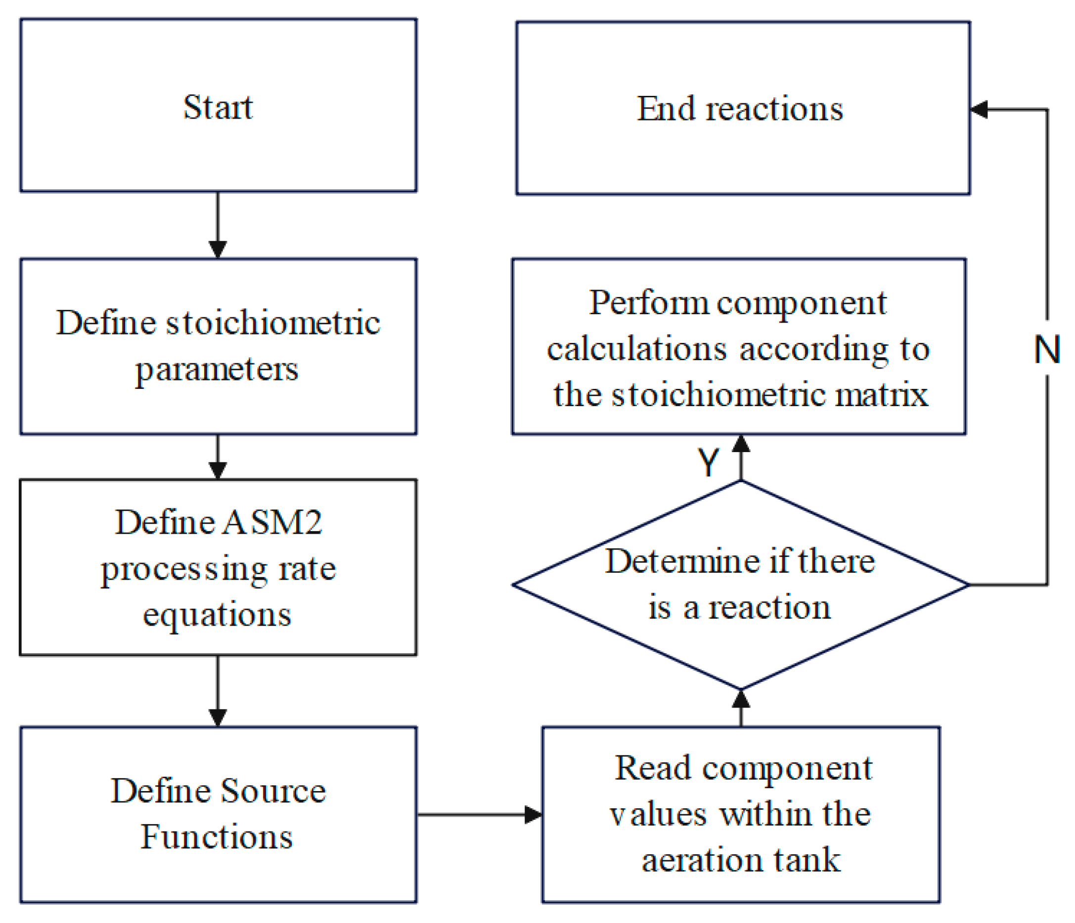
2.2. Biochemical Simulation of Activated Sludge

The activated sludge model (ASM), originally developed in 1987 by an international team of experts under the auspices of the International Water Association, has evolved to include several advanced variants, such as ASM2 and ASM2d [14]. In this study, the ASM2 model was employed to comprehensively simulate biochemical mass transfer processes in aeration tanks. ASM2 accounts for key biological processes, including organic matter degradation, nitrification, denitrification, and biological phosphorus removal. This study draws on the work of Henze [14], who defined 19 soluble and particulate components, their kinetic parameters, and the primary biochemical reactions in his foundational text. The ASM2 model represents the relationships among substance concentrations, reaction rates, kinetic parameters, and stoichiometric coefficients using a matrix format. This structure enables precise computational implementation through coding algorithms [15]. By incorporating these features, ASM2 provides a robust framework for modeling complex interactions within wastewater treatment systems, supporting the accurate simulation of aeration tank performance.

2.3. Methods for Assessment of Wastewater Quality

The wastewater treatment industry relies on various indicators to evaluate the performance of treatment systems. The ASM2 model facilitates the quantitative calculation of key water quality indicators, using simplified relationships between components as outlined by JB Copp [16]. In this study, the denitrification product (S_N2) and total suspended solids (X_TSS) from

Table 1. Components of Each Constituent in the Calculation Process of Evaluation Indicators.

Component	Number	Symbol	Definition
Dissolved components	1	$S_A$	Fermentation products (acetate)
	2	$S_{ALK}$	Bicarbonate alkalinity
	3	$S_F$	Readily biodegradable substrate
	4	$S_I$	Inert, non-biodegradable organics
	5	$S_{N_2}$	Dinitrogen (N), 0.78 atm at 20 °C
	6	$S_{NH4}$	Ammonium
	7	$S_{N{O}_3}$	Nitrate (plus nitrite)
	8	$S_{O_2}$	Dissolved oxygen
	9	$S_{P{O}_4}$	Phosphate inert
Particulate components	10	$X_{AUT}$	Autotrophic, nitrifying biomass
	11	$X_H$	Heterotrophic biomass
	12	$X_I$	Inert, non-biodegradable organics
	13	$X_{MeOH}$	“Ferric-hydroxide” (Fe(OH)3)
	14	$X_{MeP}$	“Ferric-phosphate” (FePO4)
	15	$X_{PAO}$	Phosphorus-accumulating organisms
	16	$X_{PHA}$	Organic storage products of PAO
	17	$X_{PP}$	Stored poly-phosphate of PAO
	18	$X_S$	Slowly biodegradable substrate
	19	$X_{TSS}$	Particulate material as a model component

were treated as fixed values, while the remaining 17 components were modeled and converted into COD and other evaluation metrics. The corresponding calculation formulas are as follows:

$$C_{COD}=S_A+S_F+S_I+X_I+X_S+X_H$$

(6)

$$C_{TN}=X_I\times i_{NXI}+X_S\times i_{NXS}+(X_H+X_{PAO}+X_{AUT})\times i_{NBM}+S_{N{H}_3}+(S_F+S_I)\times i_{NSI}+S_{N{O}_3}$$

(7)

$$C_{N{H}_3}=S_{N{H}_3}$$

(8)

$$C_{TP}=X_S\times i_{PXS}+X_I\times i_{PXI}+S_{P{O}_4}$$

(9)

$$C_{DO}=S_{O_2}$$

(10)

2.4. Biochemical Mass Transfer Model

CFD has been widely used to analyze and model fluid flow by solving the Navier–Stokes equations. In this study, changes in the concentrations of 19 constituents within the aeration tank were computed using a defined source term S_i during the flow process [17,18]. The flow rate of the aeration equipment was converted into the oxygen input velocity at the aeration holes, forming the basis for the numerical calculation model. This model does not account for reoxygenation occurring at the free surface of the water body [19]. The turbulence behavior was simulated using the standard k-ϵ model, while the multiphase flow was described using the MIXTURE model, where wastewater represents the primary liquid phase and sludge serves as the secondary solid phase. In calculating the transport equations for the constituents, the diffusion flux $\overline{J_i}$ was determined using the following formula [18]:

$$\overline{J_i}=-(\rho D_{i,m}+{\displaystyle \frac{{\mu }_t}{S_{C_t}}})\nabla Y_i-D_{i,T}{\displaystyle \frac{\nabla T}{T}}$$

(11)

where $D_{i,m}$ represents the diffusion coefficient of the component, subscript $i$ denotes the component index and $m$ is the mass of the component, ${\mu }_t$ is the turbulent viscosity, $S_{c_t}$ refers to the turbulent Schmidt number, $Y_i$ indicates the mass fraction of component $i$, $D_{i,T}$ denotes the temperature diffusion coefficient of component $i$, and $T$ represents the temperature.

The biochemical mass transfer model was developed using the SOURCE function [20]. Figure 1 illustrates the flowchart for the secondary development of Fluent, enabling its integration with the ASM2 model. The source term is defined using the custom function library’s DEFINE_SOURCE (XX, c, t, dS, eqn), while the mass fraction of components is read using the macro C_YI(c, t, 0). The calculation of the source term follows the equations specified in the ASM2 model [14]. To minimize computational time during the source term calculation, the component transport model is initially disabled after the source term is defined. The Mixture model is then employed to stabilize the internal flow conditions. Once this steady-state is achieved, the component transport model is re-enabled, and the source term is activated to calculate the biochemical reactions [10].

3. Results and Discussion

3.1. CFD Modeling and Analysis of Aeration Tank

To analyze the internal flow field characteristics of the aeration tank, this study establishes a CFD Fluent analysis model for the aeration tank. This is achieved by observing the calculation results in the form of streamline plots, contour plots, and line graphs.

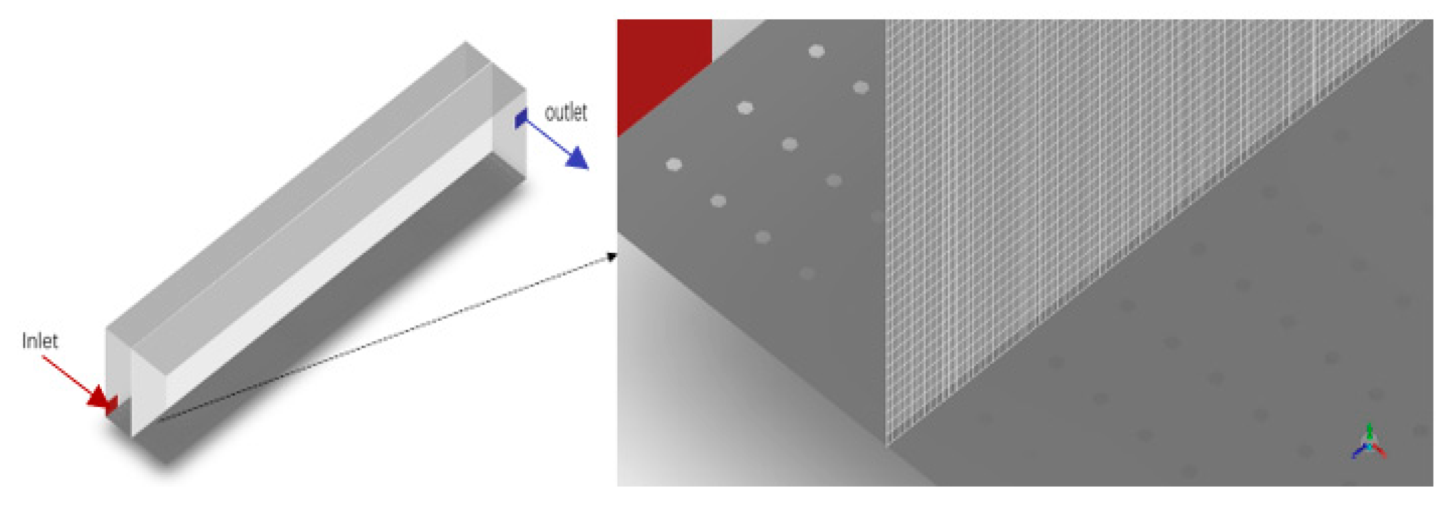
3.1.1. Geometric Modeling and Grid Generation

The aeration tank is 25 m long, 6 m wide, and 6.5 m high, as shown in Figure 2, with flat and straight walls. Considering the high precision requirements for subsequent biochemical mass transfer model calculations of the aeration tank, a structured grid is used to establish the component transport model and two-phase flow model. Figure 3 shows the distribution of aeration holes at the bottom of the aeration tank, where the aeration holes marked in red have a diameter of 0.08 m.

3.1.2. Boundary Conditions and Initial Settings

The inlet of the aeration tank is set as the velocity inlet, whereas the outlet is configured as a pressure outlet. The primary boundary conditions and initial settings are presented in

Table 2. Initial Computational Settings for the Aeration Tank.

Wastewater Inflow Velocity (m/s)	Sludge Inflow Velocity (m/s)	Aeration Velocity (m/s)	Turbulence Intensity	Total Time(s)	Number of Iterations	Convergence Criteria
0.7	0.6	0.096	10%	3600	50	<10−3

. The velocities for the sewage inlet, sludge inlet, and aeration tank aeration are calculated based on the ratio of the actual project flow rate to the inlet area.

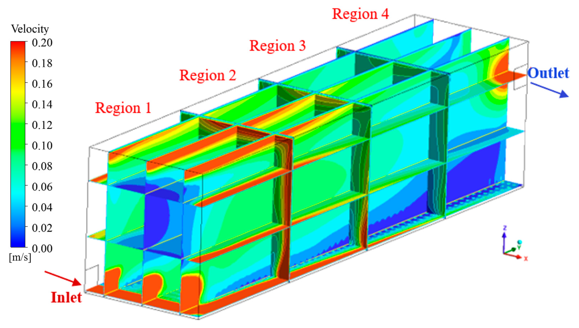
3.1.3. Analysis of Wastewater Flow Field

The grid sizes for the aeration tank are set to 0.01 m, 0.02 m, 0.025 m, 0.05 m, 0.1 m, and 0.2 m, with each volume growth rate being identical. The outlet velocities are compared across four sets of grid sizes, with the specific values shown in

Table 3. Grid Independent Flow Velocity Results.

Grid Size(m)	Flow Velocity(m/s)
0.025	0.191
0.05	0.196
0.1	0.194
0.2	0.180

.

As shown in Table 3, the flow velocity shows minimal variation for grid sizes ranging from 0.025 m to 0.1 m, with the relative velocity error remaining below 5%. However, for grid sizes outside this range, significant discrepancies in velocities are observed. To balance computational time with the accuracy of the results, a grid size of 0.1 m was chosen. The shape and aeration method of the canal aeration tank in this study are similar to those investigated by Moullec et al. [21], and the simulated flow conditions closely align with their findings, confirming the reliability of the numerical model.

Figure 4 shows the internal flow field of the aeration tank, represented by streamlines. It can be seen that the wastewater exhibits rotational flow within the tank, with the rear section affected by high-velocity airflow at the bottom, generating significant vortices. While these vortices help achieve a more uniform distribution of components towards the end of the tank, they also cause the backflow of partially treated wastewater. This secondary aeration effect leads to energy loss [22]. To further quantify this impact, we calculated the average turbulent kinetic energy at the cross-section where the vortex occurs, which is 0.002003 m²/s². At the end of the recirculation zone, the turbulent kinetic energy decreases to 0.00016 m²/s², indicating that the local turbulent kinetic energy loss rate reaches 92.01% during the vortex development process. This significant decline in turbulent kinetic energy suggests that energy dissipation within the vortex region is considerable, which may exacerbate local energy losses, thereby affecting the flow field stability and overall efficiency of the aeration system.

Figure 5 shows the velocity contour plots of wastewater at three horizontal and three vertical sections, with the flow regions divided into four zones based on the velocity at the bottom of the aeration tank. In Region 1, there is virtually no low-velocity flow (below 0.02 m/s), as indicated by the blue areas in Figure 5. In Region 2, low-velocity flow begins to appear at the tank’s bottom. As the wastewater moves into Region 3, the low-velocity flow at the bottom progressively develops and expands. In Region 4, the flow velocity at the bottom decreases significantly, creating a large low-velocity flow area.

The results of the above flow field analysis revealed severe attenuation of the flow velocity at the bottom of the aeration tank and the presence of recirculation, which leads to a reduction in aeration efficiency. These findings provide important insights into the subsequent optimization of aeration processes.

3.2. Aeration Tank Mass Transfer Model

To quantitatively analyze the water quality within the aeration tank, this study developed and calibrated a biochemical mass transfer model through the secondary development of Fluent. A comprehensive analysis was conducted using five water quality assessment indicators: dissolved oxygen (DO), chemical oxygen demand (COD), total phosphorus (TP), total nitrogen (TN), and ammonium nitrogen (NH₄⁺-N) within the aeration tank.

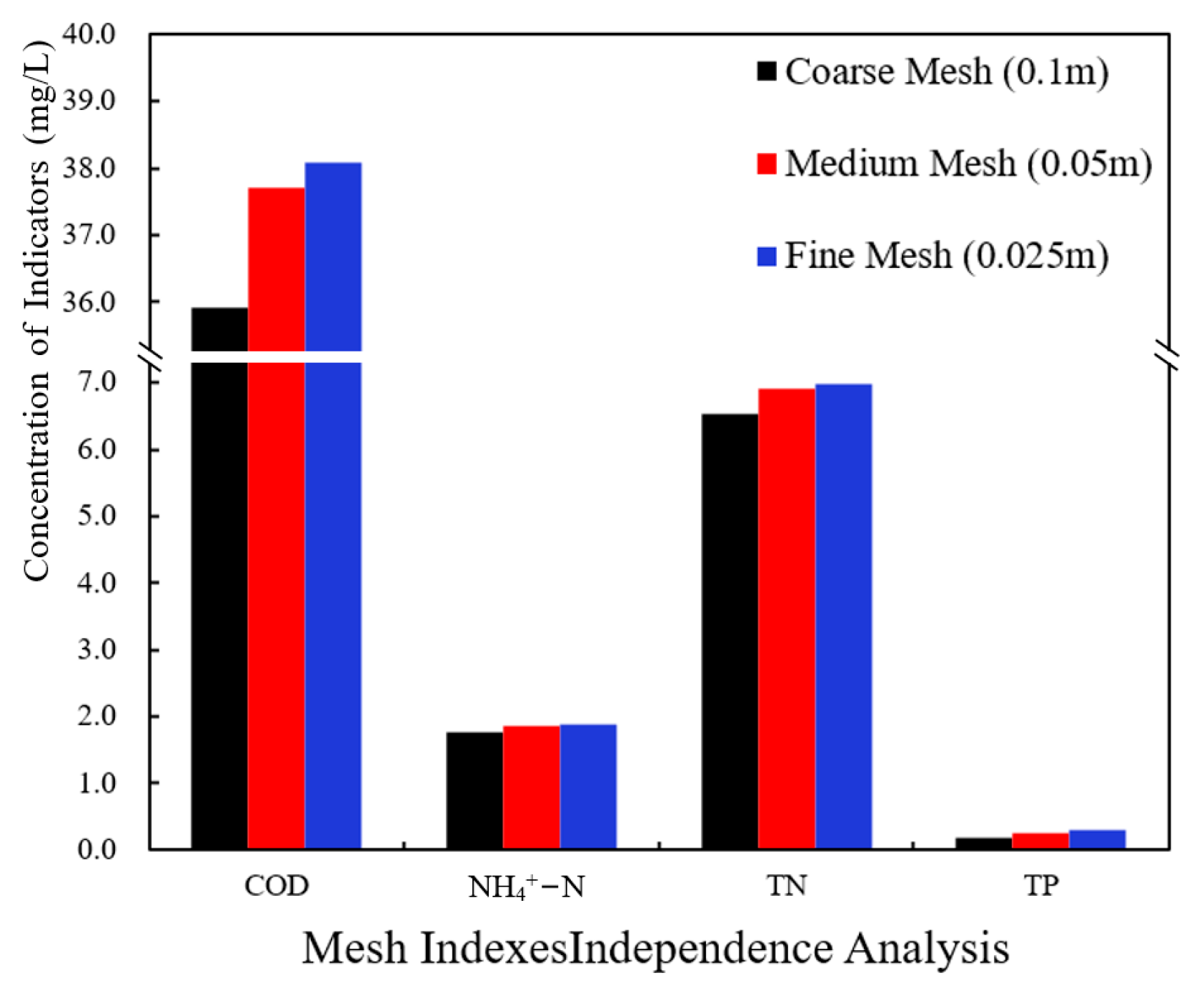
3.2.1. Grid Independence Analysis

In the ASM2-CFD coupled model, the influent concentrations at the wastewater tank inlet are as follows: COD 366.17 mg/L, NH₄⁺-N 8.95 mg/L, TN 35.69 mg/L, and TP 1.45 mg/L. All other boundary conditions remain the same as in the previous chapter. To ensure that the computational results are not affected by grid resolution, a grid independence study was conducted using a grid refinement ratio of 2 under the assumption of second-order accuracy. Three different grid sizes were selected: Coarse Grid (0.2 m), Medium Grid (0.1 m), and Fine Grid (0.05 m). The simulations were performed under identical boundary conditions, solver settings, and convergence criteria to compute the key pollutant indicators (COD, NH₄⁺-N, TN, and TP). The results are shown in Figure 6. Analysis indicates that the relative differences between the Fine and Medium grids are COD:1.02%; NH₄⁺-N:0.81%; TN:1.06%. The variation in TP is not considered a primary reference due to its small magnitude. Since all errors are below 2%, the solution is considered grid-independent, meaning further grid refinement does not significantly impact the results. Considering both computational accuracy and efficiency, the Medium Grid (0.1 m) was selected for subsequent simulations.

3.2.2. Calibration of the Biochemical Mass Transfer Model

Table 4. Effluent water quality table.

Test Items	Test Methods	Results (mg/L)
COD	Dichromate Method	33.99
NH4+-N	Nessler’s Reagent Spectrophotometric Method	1.62
TN	Alkaline Persulfate Digestion UV Spectrophotometric Method	6.28
TP	Ammonium Molybdate Spectrophotometric Method	0.16
Suspended Solids	Gravimetric Method for Determination of Suspended Solids	9

shows the actual effluent quality results of the wastewater treatment system shown in Figure 7 [23]. The system continuously treats a mixture of domestic wastewater from township residents (including nearby rural areas and commercial complexes) and industrial wastewater from industrial parks, primarily originating from the metal processing and mechanical surface treatment industries. The limitation for wastewater pollutants is based on the national standard “Quality Standards for Sewage Discharged into Urban Sewers” [24].

If the default water quality analysis parameters in the ASM2 model are used, the calculated TP concentration error can reach 60%. Analysis indicates that this discrepancy is primarily due to the significant influence of temperature on the components of the activated sludge reaction process, which is consistent with the findings reported by Chen et al. [25,26,27]. To improve model accuracy, previous studies have explored parameter modifications. For instance, Tiar S M et al. achieved good results in modifying the maximum heterotrophic growth rate and the heterotrophic decay coefficient in the ASM model [28]. As shown in Equation (9), the parameters affecting TP are $X_{\mathrm{s}}$, $X_I$, and $S_{P{O}_4}$, of which $S_{P{O}_4}$ appears to have the greatest impact. The observation of the ASM2 mass transfer process suggests that a decrease in the PHA saturation coefficient $K_{PHA}$ will reduce the rate of the $X_{PAO}$ aerobic growth process, thereby decreasing $S_{P{O}_4}$. Conversely, an increase in the polyphosphate saturation coefficient $K_{PP}$ will reduce the storage process rate of $X_{PHA}$, thus decreasing $S_{P{O}_4}$. Based on this analysis, the value of $K_{PHA}$ was adjusted from the default 0.01 to 0.008, and $K_{PP}$ from the default 0.01 to 0.016. Figure 8 compares the measured values and the simulation results using the default and corrected parameters, demonstrating that the accuracy of the calculated indicators exceeds 85% after the adjustments.

3.2.3. Effect of Original Scheme

Figure 9 shows the concentration contour maps for the five key evaluation indices obtained using the corrected parameters at three horizontal sections: Bottom, Middle, and Top. Each evaluation index is presented in its direct dimensional form. In Fluent, the components were inputted as percentages. For example, the COD concentration at the inlet was 37.93%, which corresponds to an actual inlet concentration of 367 mg/L. The calculation method is as follows:

$$C_{COD}=\left(S_A+S_F+S_I+X_I+X_S+X_H\right)\times {\displaystyle \frac{367}{37.93\%}}$$

(12)

From Figure 9a, the dissolved oxygen (DO) concentration distribution contour map shows a trend similar to the results reported by Shao et al. [29]. The DO concentration is highest near the outlet in the bottom section, and there is also an increasing trend near the outlet in the top section. The dissolved oxygen (DO) concentration at the outlet of the aeration tank was measured to be above 3 mg/L. For the wastewater treatment plant analyzed in this study, the optimal DO concentration range is 2.0–2.5 mg/L [30]. Excessive DO can negatively affect the denitrification process by inhibiting the activity of denitrifying bacteria, which leads to reduced nitrogen removal efficiency. Additionally, excessive aeration may hinder the degradation of refractory organic matter and accelerate sludge aging due to increased endogenous respiration of microorganisms under high DO conditions. From the DO distribution in different sections of the aeration tank (Figure 9a), it can be observed that excessive DO occurs at the tank’s end because biological COD degradation is nearly complete there. This reduced bacterial oxygen consumption results in higher residual DO concentrations. Consequently, the uniform aeration strategy leads to excessive aeration in the latter section, causing energy waste and increased operational costs.

From Figure 9b, the chemical oxygen demand (COD) concentration contour map shows that the COD concentration rapidly decreases from 259 to 370 mg/L to 74–220 mg/L after the sewage enters the aeration tank. Because under the conditions of DO ≥ 0.5–1 mg/L, the ASM model shows that oxygen supply no longer significantly limits the metabolism of heterotrophic and autotrophic bacteria, thus accelerating the decrease in COD. Additionally, the COD concentration near the walls is higher at all sections. Based on the velocity streamlines, it can be observed that the sewage flows in a rotating manner in this area, leading to lower kinetic energy near the walls and poor mixing of the sewage, which results in this phenomenon.

From Figure 9c, the ammonium nitrogen (NH₄⁺-N) concentration contour map shows that the NH₄⁺-N concentration at the bottom monitoring section rapidly decreases from the inlet to 11–25 mg/L. The overall trend in the middle and top monitoring sections is similar, with a noticeable concentration decrease in the middle of the sewage tank, which is consistent with the results of the COD and DO concentration distribution maps.

From Figure 9d, the total nitrogen (TN) concentration contour map indicates that the TN concentration in sewage rapidly drops to 30–50 mg/L with aeration. Because of sufficient oxygen in the aeration tank, the overall TN concentration change was relatively stable. The TN concentration slightly increased with distance from the aeration holes, which aligns with descriptions of TN distribution in the upper, middle, and lower layers of the aeration tank by Zhou et al. [31].

From Figure 9e, the total phosphorus (TP) concentration contour map shows a distribution similar to that of NH₄⁺-N. The TP concentration was lower at the bottom monitoring section and rear of the sewage tank. The TP concentration results in different sections indicate that the current aeration method effectively removed TP.

The results of the above biochemical mass transfer model characterize the distribution and interrelationships of various evaluation indicators at different locations within the aeration tank, which provide an important basis for the subsequent optimization and improvement of the aeration scheme.

3.3. Aeration Rate Optimization

To further optimize the energy consumption of the aeration tank and enhance aeration efficiency, this study proposes a quantifiable metric that evaluates the relationship between aeration and purification efficiency by calculating the pollutant removal capacity per unit volume (${\text{m}}^3$) of aeration within a unit time. This approach allows the assessment of the advantages and disadvantages of aeration velocities in different regions. The benefits of the aeration optimization scheme are described by the treatment capacity per unit volume of aeration and the overall purification efficiency of the aeration tank.

3.3.1. Optimization Based on Component Concentration

The distribution cloud map of the evaluation indicators indicates a clear stratification among the various metrics. Therefore, regions with different aeration velocities can be delineated to minimize the energy loss in the aeration tank. Figure 10 presents three distinct partitioning schemes, described as a, b, and c.

For each delineated region, the aeration volume per unit volume (m³) during the wastewater treatment process can be expressed as the removal capacity of pollutants ${\mathsf{\eta }}_a$,

$${\mathsf{\eta }}_i=({\displaystyle \frac{C_{S_i}-C_{S_{i+1}}}{C_{S_i}}})\times 100\%$$

(13)

$${\mathsf{\eta }}_{a_i}={\displaystyle \frac{{\mathsf{\eta }}_i}{v_i\times A_i}}$$

(14)

where ${\mathsf{\eta }}_i$ represents the purification efficiency of region $i$, $C_{S_i}$ is the average concentration of indicator $S_i$ obtained from simulation calculations (i = 1~4), $v_i$ is the aeration rate of region $i$, $A_i$ is the aeration orifice area of region $i$, and ${\mathsf{\eta }}_{a_i}$ represents the purification effect of the aeration volume per unit volume in region $i$.

Indicator ${\mathsf{\eta }}_a$ reflects the ability of the aeration volume per unit volume of the aeration tank to remove pollutants. The higher the value of ${\mathsf{\eta }}_a$, the better the aeration effect. The value of ${\mathsf{\eta }}_a$ for each region is calculated, and the ratio of pollutants to aeration speed in the region with the highest ${\mathsf{\eta }}_a$ is established as the optimal ratio, which is then used to adjust the aeration speeds in other regions. Assuming that region 1 has the highest ${\mathsf{\eta }}_a$, the adjustment process for the aeration speed in region 2 can be expressed as,

$$V_2={\displaystyle \frac{V_1}{4}}\times {\displaystyle \sum _{j=1}^4{\left(\frac{C_{S_2}}{C_{S_1}}\right)}_j}$$

(15)

where $V_1$ represents the aeration speed in Region 1, $C_{S_1}$ and $C_{S_2}$ denote the concentrations of the evaluation indicators at monitoring sections 1 and 2, respectively. Here, j = 1–4 corresponds to the COD, TP, TN, and NH₄⁺-N.

Using the biochemical mass transfer model, simulations were conducted for the three models after the speed adjustments, as depicted in Figure 10, and the results were compared with those of uniform aeration. The aeration purification effects regarding the four evaluation indicators: COD, TP, TN, and NH₄⁺-N are illustrated in Figure 11 below.

As shown in Figure 11, the aeration effects of schemes a, b, and c significantly exceed those of the original scheme, highlighting the necessity of dividing the aeration tank into specific zones. When the aeration tank is divided into four regions, the purification effect of aeration is optimized. This division method corresponds to the diffusion phenomenon observed in the low-flow regions of the flow field, indicating that the flow field influences aeration efficiency. The calculated ${\mathsf{\eta }}_a$ values for each partition in scheme b are presented in

Table 5. Evaluation of Unit Volume Aeration Treatment Capacity for Scheme b (m⁻³h).

Region	COD	NH4+-N	TN	TP	Average
1	2.83	2.78	2.92	3.07	2.90
2	2.85	2.83	2.89	2.97	2.88
3	1.19	1.17	1.24	1.32	1.23
4	1.38	1.36	1.43	1.53	1.43
Average	2.06	2.03	2.12	2.23	2.11
Improved rate	14.97%	14.72%	15.53%	16.58%	15.47%

.

From the table, it is evident that with the implementation of Scheme b, the overall average values of COD and other indicators in the wastewater treatment plant across the four zones improved by over 14.7%. Figure 12 compares the DO distribution of the original scheme (left) with that of scheme b (right). The DO distribution in Scheme b is more uniform and has a lower concentration than the initial scheme, indicating that the aeration speed in the aeration tank has been effectively optimized.

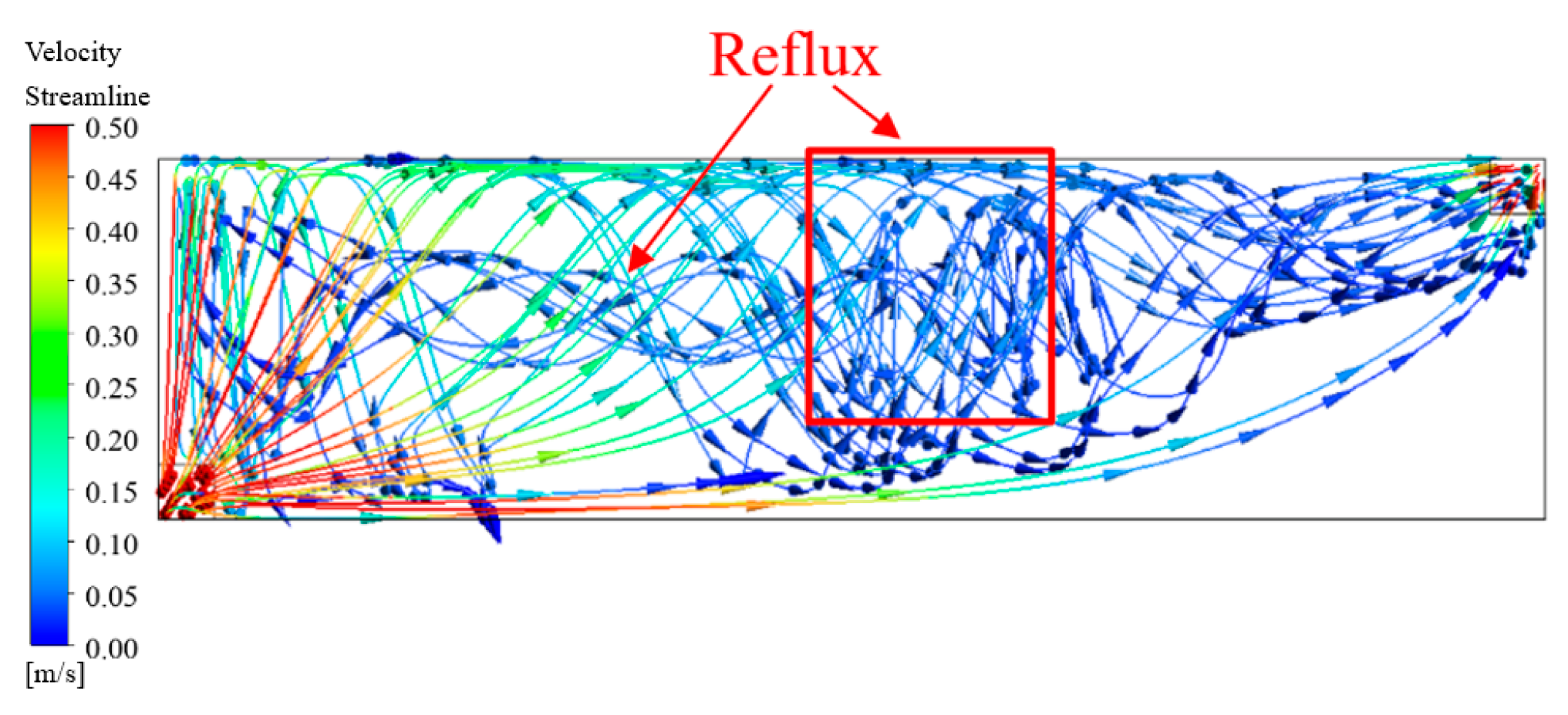
3.3.2. Optimization Considering Reflux Effects

Table 5 indicates that the unit volume aeration treatment capacity of Zone 3 in Scheme b is lower than that of the other zones. An analysis of the computational results reveals that Scheme b does not adequately consider the impact of the high-velocity gas flow generated by aeration on the flow field of wastewater within the aeration tank. As illustrated in Figure 13, the progressively reduced aeration velocity within the tank leads to premature recirculation, significantly diminishing the rotational flow of wastewater at the rear end of the aeration tank. This results in insufficient reaction of the wastewater and a decrease in the purification efficiency.

Considering both the positive effects of recirculation on mixing and the negative impacts of secondary aeration, it is deemed more appropriate for recirculation to occur at the front end of Zone 3. According to the Bernoulli equation, as the fluid flow velocity increases, the pressure decreases. Thus, the aeration speed in Zone 4 can be increased to create a pressure differential and delay the occurrence of vortices. Given that increasing the aeration speed beyond that of the initial scheme may pose unpredictable risks to the strength of the aeration piping, the aeration speed is set to 0.096 m/s, which is consistent with the initial scheme, forming scheme d, as shown in

Table 6. Aeration Speeds for Each Region in Scheme d (m/s).

Aeration Schemes	Region 1	Region 2	Region 3	Region 4	Aeration Flow (m3/s)
Scheme b	0.096	0.070	0.059	0.046	0.30
Scheme d	0.096	0.070	0.059	0.096	0.35

. The biochemical mass transfer model was employed to simulate Scheme b, and its ${\mathsf{\eta }}_a$ values are presented in

Table 7. Evaluation of Unit Volume Aeration Treatment Capacity for Scheme d (m⁻³h).

Region	COD	NH4+-N	TN	TP	Average
1	2.40	2.49	2.36	2.36	2.40
2	1.88	1.91	1.86	1.86	1.88
3	4.46	4.51	4.44	4.44	4.46
4	0.52	0.55	0.50	0.50	0.52
Average	2.13	2.11	2.16	2.22	2.15
Improved rate	29.04%	33.31%	24.90%	19.93%	26.66%

. The flow lines within the tank are shown in Figure 14, respectively.

From Table 7, it is evident that Scheme d exhibits a significant improvement in volumetric aeration treatment capacity in Region 3. Although the treatment capacities in Regions 1 and 4 are lower than those in Scheme b due to the influence of backflow, the average volumetric aeration treatment capacity across the four regions in Scheme d has increased from 14.7% in Scheme b to over 19.9%. Figure 14 demonstrates that the backflow in Scheme d is significantly delayed compared to Scheme b, which enhances the stirring effect in the latter stages of the aeration tank and results in improved effluent quality in Scheme d.

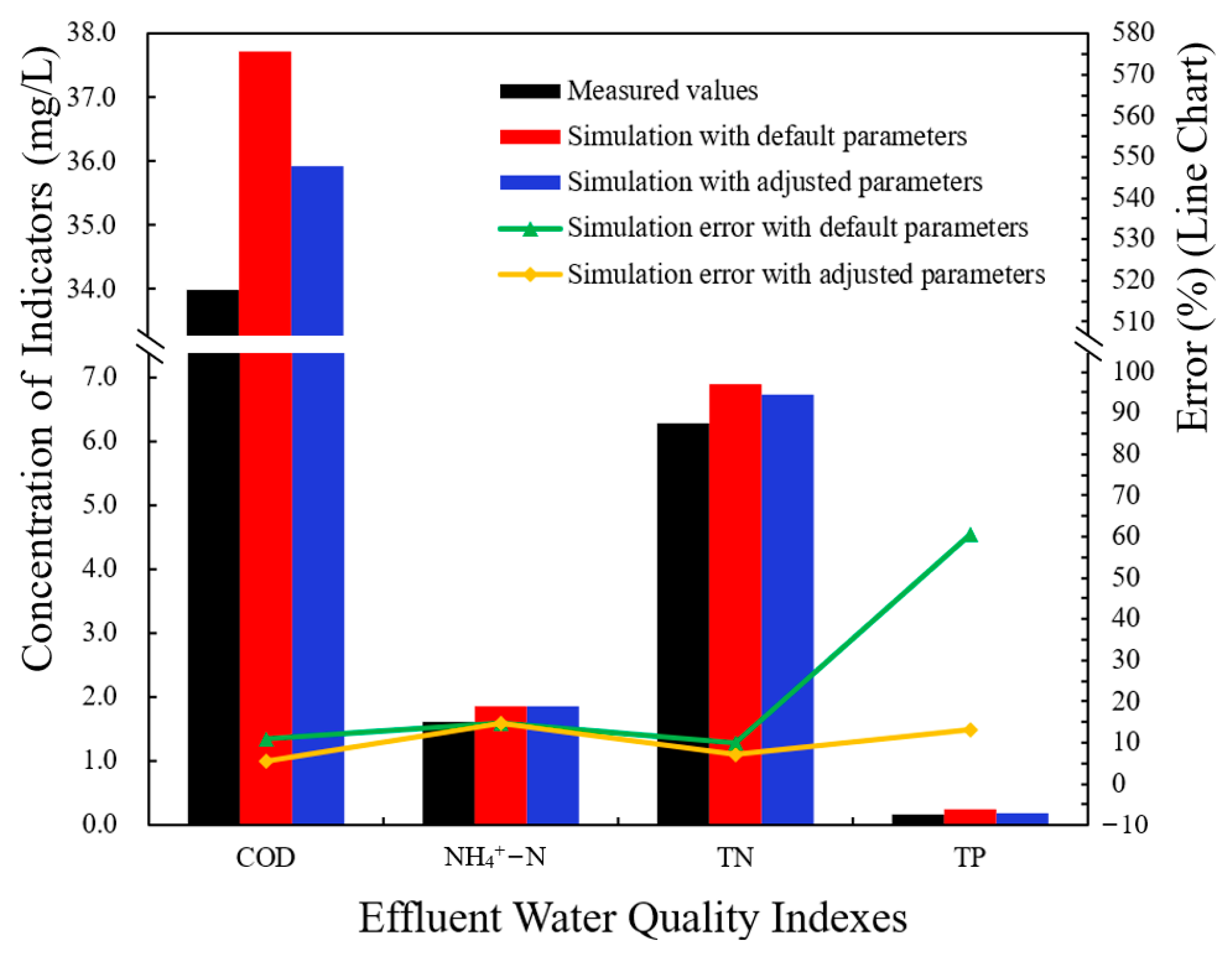
3.3.3. Analysis of Effluent Water Quality

The optimization of aeration speed is predicated on the requirement that the effluent quality from the aeration tank meets the specified standards. The purification efficiencies of the three proposed schemes for the four evaluation indicators are shown in Figure 15.

From Figure 15, it is evident that under a 28% reduction in aeration volume, Scheme b maintains the purification efficiency loss of various evaluation indicators within 8%. In contrast, Scheme d, with a 16% reduction in aeration volume, achieves a purification efficiency loss of less than 5.5%. This indicates that both schemes have a minimal impact on the effluent quality of the aeration tank, meeting the Class A standard outlined in China’s “Discharge Standard of Pollutants for Municipal Wastewater Treatment Plants” [24], which specifies COD ≤ 50 mg/L, TN ≤ 15 mg/L, NH₄⁺-N ≤ 5 mg/L, and TP ≤ 0.5 mg/L. Therefore, while the original scheme provides the best effluent quality, Scheme b demonstrates superior performance from the perspective of energy consumption optimization while still meeting the effluent quality requirements. Meanwhile, if the goal is to minimize the loss of purification efficiency while optimizing the energy consumption, Scheme d is more appropriate.

4. Conclusions

In this study, we successfully developed a biochemical mass transfer model for aeration tanks and applied it to simulate the performance of a real-world sewage aeration system. Calibration with measured data demonstrated an accuracy exceeding 85%. Based on the computational results, a more cost-effective aeration strategy was proposed and validated, leading to the following key insights:

(1)

Flow dynamics—Under bottom microporous aeration and lateral inflow, wastewater exhibited rotational flow patterns within the rectangular aeration tank. As the flow progressed, velocity at the tank’s bottom gradually decreased, becoming turbulent at 17 meters from the inlet and initiating recirculation.

(2)

From the component distribution contour map, it can be observed that the distribution of dissolved oxygen (DO) has a clear spatial coupling relationship with the concentration distributions of COD, TN, NH₄⁺-N, and TP. Furthermore, maintaining the dissolved oxygen concentration is one of the highest energy consumption aspects in wastewater operation. Therefore, DO can be considered a key indicator for evaluating the water quality of the wastewater tank. In Scheme I, the DO distribution within the tank is uniform, which can be regarded as the optimal operating condition.

(3)

Recirculation control—Adjusting aeration velocities by zones allowed control of recirculation locations. When recirculation occurred in the tank’s front section, outlet concentrations of COD, NH₄⁺-N, TN, and TP improved by 2.1%, 2.14%, 2.01%, and 1.87%, respectively, compared to recirculation at the rear. This highlights the uneven component distribution as flow diminishes within the tank.

(4)

Optimization outcomes—Two optimization schemes were proposed. One is a 28% reduction in aeration volume with an average purification efficiency loss of 7.12%. The other is a 16% reduction in aeration volume with a purification efficiency loss limited to 5.08%. These findings demonstrate that purification efficiency does not increase linearly with aeration volume, especially in zones with recirculation or low-velocity flows.

Overall, this research provides valuable empirical evidence and practical strategies for optimizing aeration in wastewater treatment plants, balancing energy efficiency and effluent quality.

References

1. Lizarralde, I.; Fernández-Arévalo, T.; Beltrán, S.; Ayesa, E.; Grau, P. Validation of a multi-phase plant-wide model for the description of the aeration process in a WWTP. Water Res. 2018, 129, 305–318. [Google Scholar] [CrossRef] [PubMed]
2. Gu, Y.; Li, Y.; Yuan, F.; Yang, Q. Optimization and control strategies of aeration in WWTPs: A review. J. Clean. Prod. 2023, 418, 138008. [Google Scholar] [CrossRef]
3. Zhou, X.; Wu, Y.; Shi, H.; Song, Y. Evaluation of oxygen transfer parameters of fine-bubble aeration system in plug flow aeration tank of wastewater treatment plant. J. Environ. Sci. 2013, 25, 295–301. [Google Scholar] [CrossRef]
4. Shah, M.P.; Rodriguez-Couto, S. (Eds.) Membrane-Based Hybrid Processes for Wastewater Treatment; Elsevier: Amsterdam, The Netherlands, 2021. [Google Scholar]
5. Goula, A.M.; Kostoglou, M.; Karapantsios, T.D.; Zouboulis, A.I. A CFD methodology for the design of sedimentation tanks in potable water treatment: Case study: The influence of a feed flow control baffle. Chem. Eng. J. 2008, 140, 110–121. [Google Scholar] [CrossRef]
6. Griborio, A.; Latimer, R.; Zhang, S.; Pitt, P.; Elmendorf, H.; Richards, T.; Porter, R. Comprehensive Approach for the Evaluation of Rectangular Primary Clarifiers at the F. In Wayne Hill Water Resources Center. In Proceedings of the 84th Annual Water Environment Federation Technical Exhibition and Conference, Los Angeles, CA, USA, 15–19 October 2011; Water Environment Federation: Alexandria, VA, USA, 2011; pp. 5298–5314. [Google Scholar]
7. Kostoglou, M.; Karapantsios, T.D.; Matis, K.A. CFD model for the design of large scale flotation tanks for water and wastewater treatment. Ind. Eng. Chem. Res. 2007, 46, 6590–6599. [Google Scholar] [CrossRef]
8. Sobremisana, A.P.; Ducoste, J.J.; de los Reyes, F.L. Combining CFD, floc dynamics, and biological reaction kinetics to model carbon and nitrogen removal in an activated sludge system. In WEFTEC 2011; Water Environment Federation: Alexandria, VA, USA, 2011; pp. 3272–3282. [Google Scholar]
9. Torregrossa, D.; Marvuglia, A.; Leopold, U. A novel methodology based on LCA+ DEA to detect eco-efficiency shifts in wastewater treatment plants. Ecol. Indic. 2018, 94, 7–15. [Google Scholar] [CrossRef]
10. Climent, J.; Basiero, L.; Martínez-Cuenca, R.; Berlanga, J.; Julián-López, B.; Chiva, S. Biological reactor retrofitting using CFD-ASM modelling. Chem. Eng. J. 2018, 348, 1–14. [Google Scholar] [CrossRef]
11. Sin, G.; Al, R. Activated sludge models at the crossroad of artificial intelligence—A perspective on advancing process modeling. Npj Clean Water 2021, 4, 16. [Google Scholar] [CrossRef]
12. Nam, K.J.; Heo, S.K.; Tariq, S.; Woo, T.; Yoo, C. Multi-agent reinforcement learning-enhanced autonomous calibration method for wastewater treatment modeling: Long-term validation of a full-scale plant. J. Water Process Eng. 2024, 59, 104908. [Google Scholar] [CrossRef]
13. Ding, M.; Zhang, S.; Wang, J.; Ye, F.; Chen, Z. Study on Spatial and Temporal Distribution Characteristics of the Cooking Oil Fume Particulate and Carbon Dioxide Based on CFD and Experimental Analyses. Atmosphere 2023, 14, 1522. [Google Scholar] [CrossRef]
14. Henze, M.; Gujer, W.; Mino, T.; van Loosdrecht, M. Activated Sludge Models ASM1, ASM2, ASM2d and ASM3; IWA Publishing: London, UK, 2015. [Google Scholar]
15. Brdjanovic, D.; Meijer, S.C.; Lopez-Vazquez, C.M.; Hooijmans, C.M.; van Loosdrecht, M.C. (Eds.) Applications of Activated Sludge Models; IWA Publishing: London, UK, 2015. [Google Scholar]
16. Copp, J.B. (Ed.) The Cost Simulation Benchmark: Description and Simulator Manual: A Product of Cost Action 624 and Cost Action 682; EUR-OP: Luxembourg, 2002. [Google Scholar]
17. Lei, L.; Ni, J. Three-dimensional three-phase model for simulation of hydrodynamics, oxygen mass transfer, carbon oxidation, nitrification and denitrification in an oxidation ditch. Water Res. 2014, 53, 200–214. [Google Scholar] [CrossRef]
18. Xu, Q.; Wan, Y.; Wu, Q.; Xiao, K.; Yu, W.; Liang, S.; Zhu, Y.; Hou, H.; Liu, B.; Hu, J.; et al. An efficient hydrodynamic-biokinetic model for the optimization of operational strategy applied in a full-scale oxidation ditch by CFD integrated with ASM2. Water Res. 2021, 193, 116888. [Google Scholar] [CrossRef]
19. Xie, H.; Yang, J.; Hu, Y.; Zhang, H.; Yang, Y.; Zhang, K.; Zhu, X.; Li, Y.; Yang, C. Simulation of flow field and sludge settling in a full-scale oxidation ditch by using a two-phase flow CFD model. Chem. Eng. Sci. 2014, 109, 296–305. [Google Scholar] [CrossRef]
20. Manual, U. ANSYS FLUENT 12.0. In Theory Guide; ANSYS Inc.: Canonsburg, PA, USA, 2009; Volume 67. [Google Scholar]
21. Le Moullec, Y.; Potier, O.; Gentric, C.; Leclerc, J.P. Flow field and residence time distribution simulation of a cross-flow gas–liquid wastewater treatment reactor using CFD. Chem. Eng. Sci. 2008, 63, 2436–2449. [Google Scholar] [CrossRef]
22. Zhang, J.; Dong, Y.; Wang, Q.; Xu, D.; Lv, L.; Zhang, G.; Ren, Z. Effects of lysed sludge reflux point on ultrasound lysis-cryptic growth in anaerobic/aerobic (A/O) wastewater treatment: Sludge reduction, microbial community, and metabolism. J. Environ. Manag. 2023, 347, 119111. [Google Scholar] [CrossRef] [PubMed]
23. Liaoning Changxin Environmental Engineering Consulting Co., Ltd. Environmental Impact Assessment Report for the Sewage Treatment Plant Project in Qilihe Economic Development Zone, Yixian County, Jinzhou; Draft for Review; Construction Unit: Management Committee of Qilihe Economic Development Zone: Jinzhou, China, 2021. [Google Scholar]
24. SAC/TC 434; Water Quality Standard for Sewage Discharged into Urban Sewage Systems: GB/T 31962-2015. China Standard Press: Beijing, China, 2015.
25. Chen, Y.; Liu, Y.; Lv, J.; Wu, D.; Jiang, L.; Lv, W. Short-time aerobic digestion treatment of waste activated sludge to enhance EPS production and sludge dewatering performance by changing microbial communities: The impact of temperature. Water Cycle 2024, 5, 5146–5155. [Google Scholar] [CrossRef]
26. Tong, L.; Xing, Z.; Gang, T.; Yang, X.; Zhi, H.; Qiu, X.; Li, X.; Wang, Z. Effects of temperature shocks on the formation and characteristics of soluble microbial products in an aerobic activated sludge system. Process Saf. Environ. Prot. 2022, 158, 158231–158241. [Google Scholar]
27. Shao, Y.; Wang, Y.; Wang, H.; Liu, G.H.; Qi, L.; Xu, X.; Zhang, J.; Liu, S.; Sun, W. Effect of operating temperature on the efficiency of ultra-short-sludge retention time activated sludge systems. Environ. Sci. Pollut. Res. 2021, 28, 39257–39267. [Google Scholar] [CrossRef]
28. Tiar, S.M.; Bessedik, M.; Abdelbaki, C.; ElSayed, N.B.; Badraoui, A.; Slimani, A.; Kumar, N. Steady-State and dynamic simulation for wastewater treatment plant management: Case study of Maghnia City, North-West Algeria. Water 2024, 16, 269. [Google Scholar] [CrossRef]
29. Fayolle, Y.; Cockx, A.; Gillot, S.; Roustan, M.; Héduit, A. Oxygen transfer prediction in aeration tanks using CFD. Chem. Eng. Sci. 2007, 62, 7163–7171. [Google Scholar] [CrossRef]
30. Xu, J.; Wang, P.; Li, Y.; Niu, L.; Xing, Z. Shifts in the microbial community of activated sludge with different COD/N ratios or dissolved oxygen levels in Tibet, China. Sustainability 2019, 11, 2284. [Google Scholar] [CrossRef]
31. Zhou, X.; Han, Y.; Guo, X. Identification and evaluation of SND in a full-scale multichannel oxidation ditch system under different aeration modes. Chem. Eng. J. 2015, 259, 715–723. [Google Scholar] [CrossRef]
Figure 1. Flowchart of ASM2 Coupling with Fluent.
Water 17 00875 g001
Figure 2. Schematic Diagram of Aeration Tank Grid Structure.
Water 17 00875 g002
Figure 3. Aeration hole distribution size chart.
Water 17 00875 g003
Figure 4. Distribution of Internal Velocity Streamlines in the Aeration Tank. (a) Three−dimensional View of the Flow Streamlines in the Aeration Tank. (b) Main View, Top View, and Left View of the Flow Streamlines in the Aeration Tank.
Water 17 00875 g004
Figure 5. Velocity Contour Plot of Aeration Tank.
Water 17 00875 g005
Figure 6. Simulation results for different grid sizes.
Water 17 00875 g006
Figure 7. Micro porous aeration experimental testing site.
Water 17 00875 g007
Figure 8. Comparison of Simulated Water Quality and Measured Water Quality.
Water 17 00875 g008
Figure 9. Concentration Distribution Contour Maps of Various Indicators in the Sewage Tank. Note: The Bottom, Middle, and Top sections are located 0.1 m, 2.5 m, and 5 m from the bottom of the aeration tank, respectively.
Water 17 00875 g009
Figure 10. Schematic Diagram of Aeration Hole Partitioning. Note: (a) divides the aeration speed of the aeration tank into three stages, (b) into four stages, and (c) into five stages.
Water 17 00875 g010
Figure 11. Comparison of Aeration Purification Effects.
Water 17 00875 g011
Figure 12. Comparison of DO distributions. Note: In each subfigure, the original scheme is shown on the left, and Scheme b is shown on the right.
Water 17 00875 g012
Figure 13. Speed Flowline Distribution in the Aeration Tank under Scheme b (35 Lines).
Water 17 00875 g013
Figure 14. Velocity Streamline Distribution in the Aeration Tank for Scheme d (35 Lines).
Water 17 00875 g014
Figure 15. Purification Efficiency of the Aeration Tank.
Water 17 00875 g015