
Managing Cyanobacteria Blooms in Lake Hume: Abundance Dynamics Across Varying Water Levels


Abstract
:1. Introduction
2. Methods
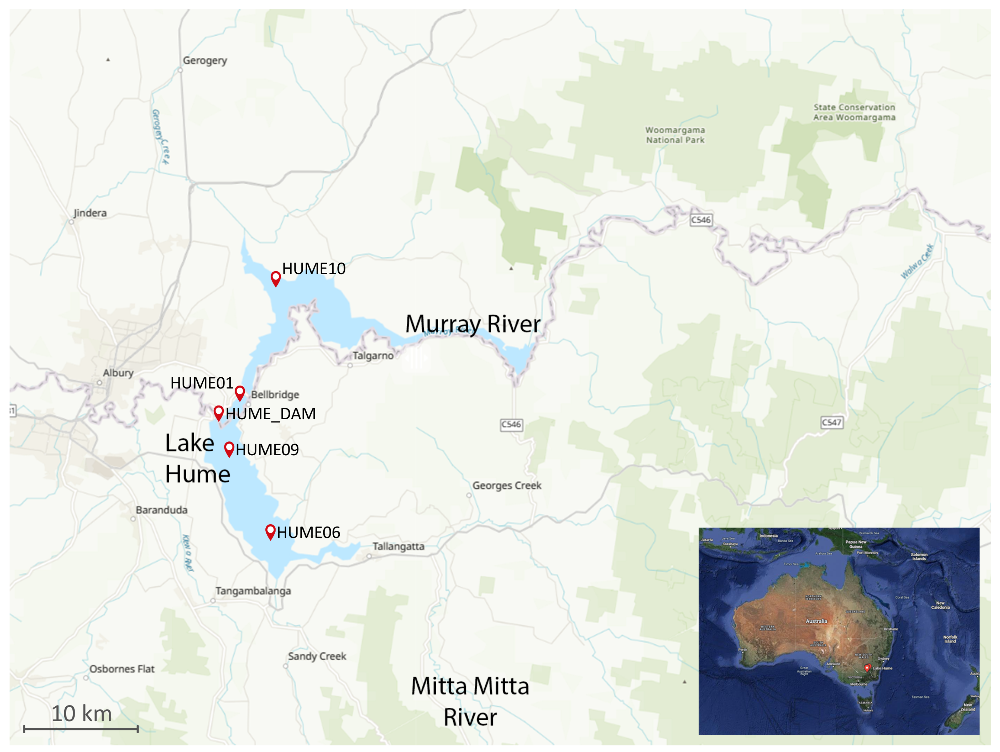
2.1. Study Site
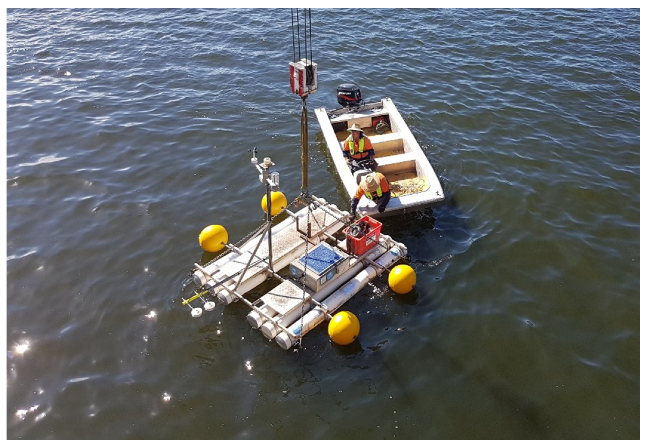
2.2. Sampling Sites and Physical Measurements
- 28 February–2 March 2017.
- 28–30 March 2017.
- 26–28 April 2017.
- 14 August 2017.
- 28 February 2018.
- 24 January 2020.
- 13 February 2020.
- 3 March 2020.
- 13 December 2020.
- 7 January 2021.
2.3. Hydrodynamic and Algal Growth Model
2.3.1. Hydrodynamic Model—Background
2.3.2. One-Dimensional Hydrodynamic Model
2.3.3. Cyanobacteria Growth Model
2.3.4. Model Simulation with Varying Water Level in the Dam
2.4. Model Setup and Input Data
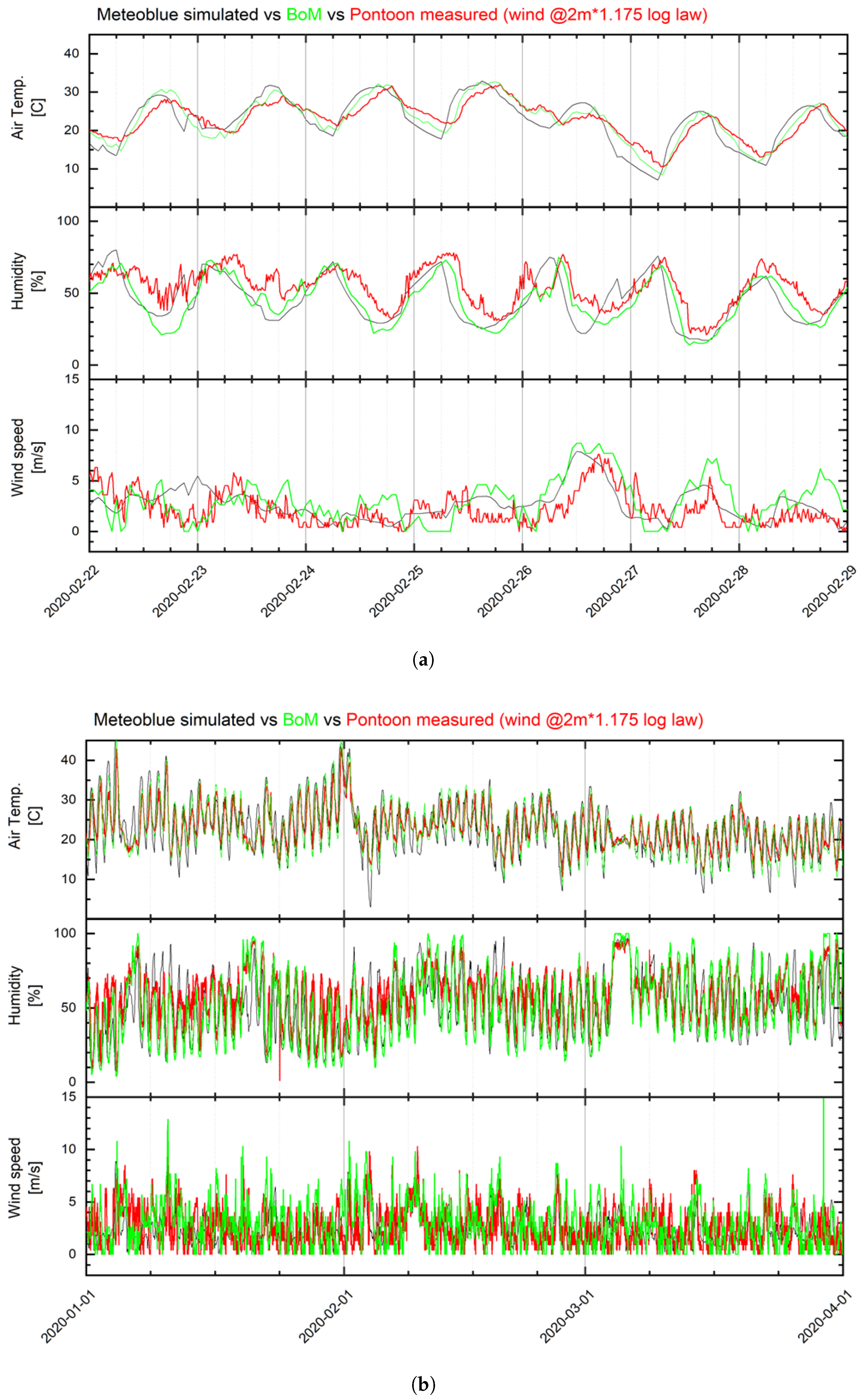
Meteorological Data
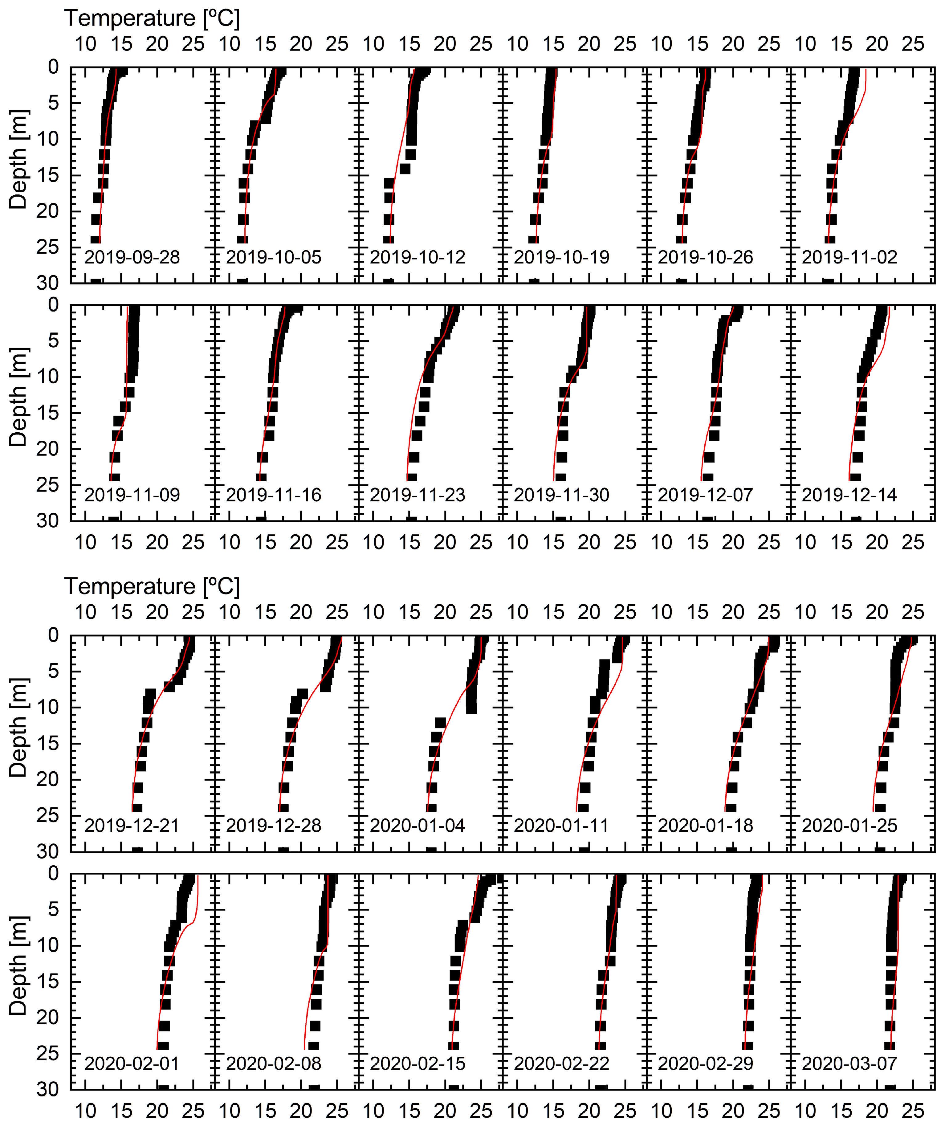
2.5. Model Calibration
3. Results
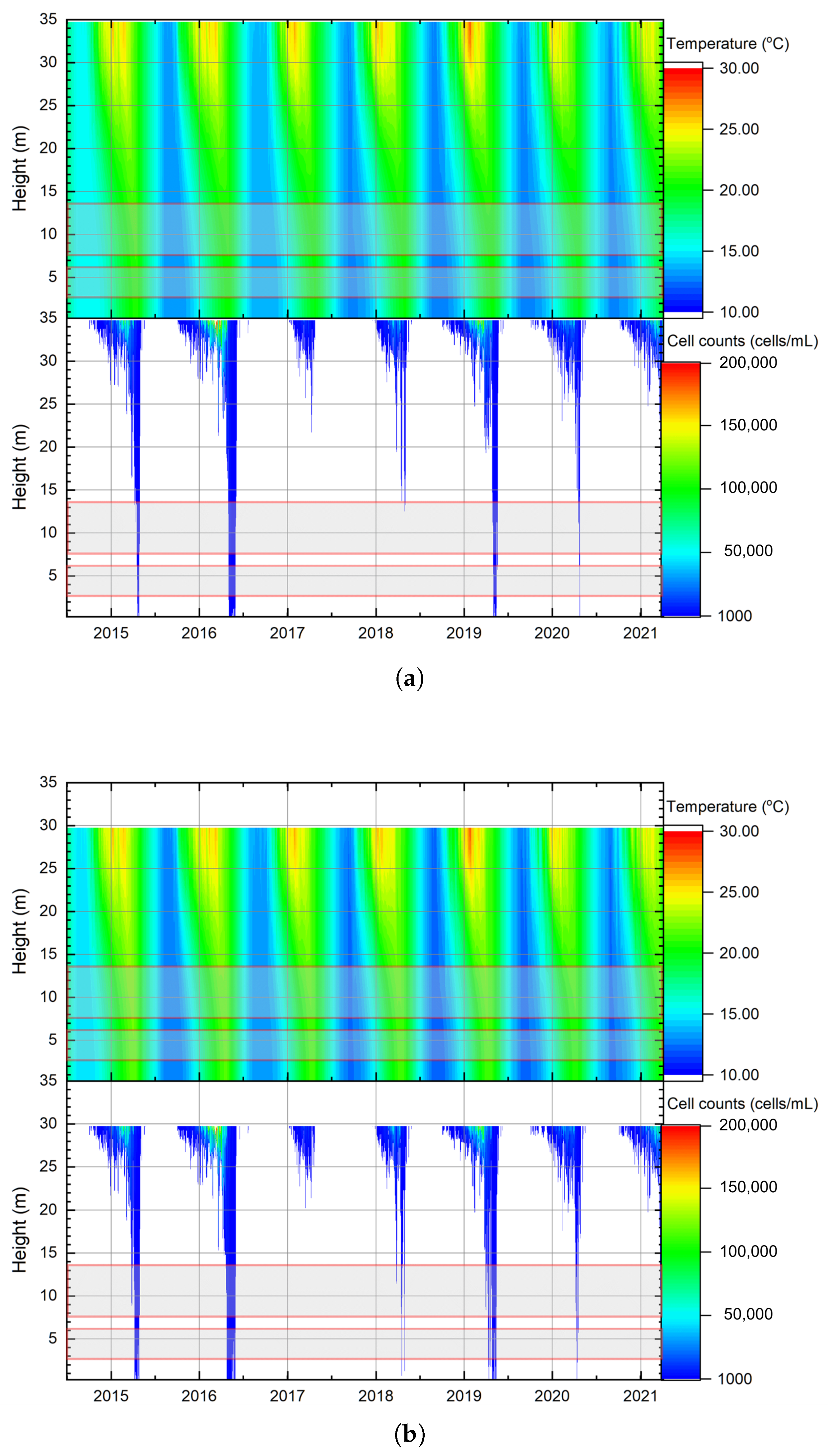
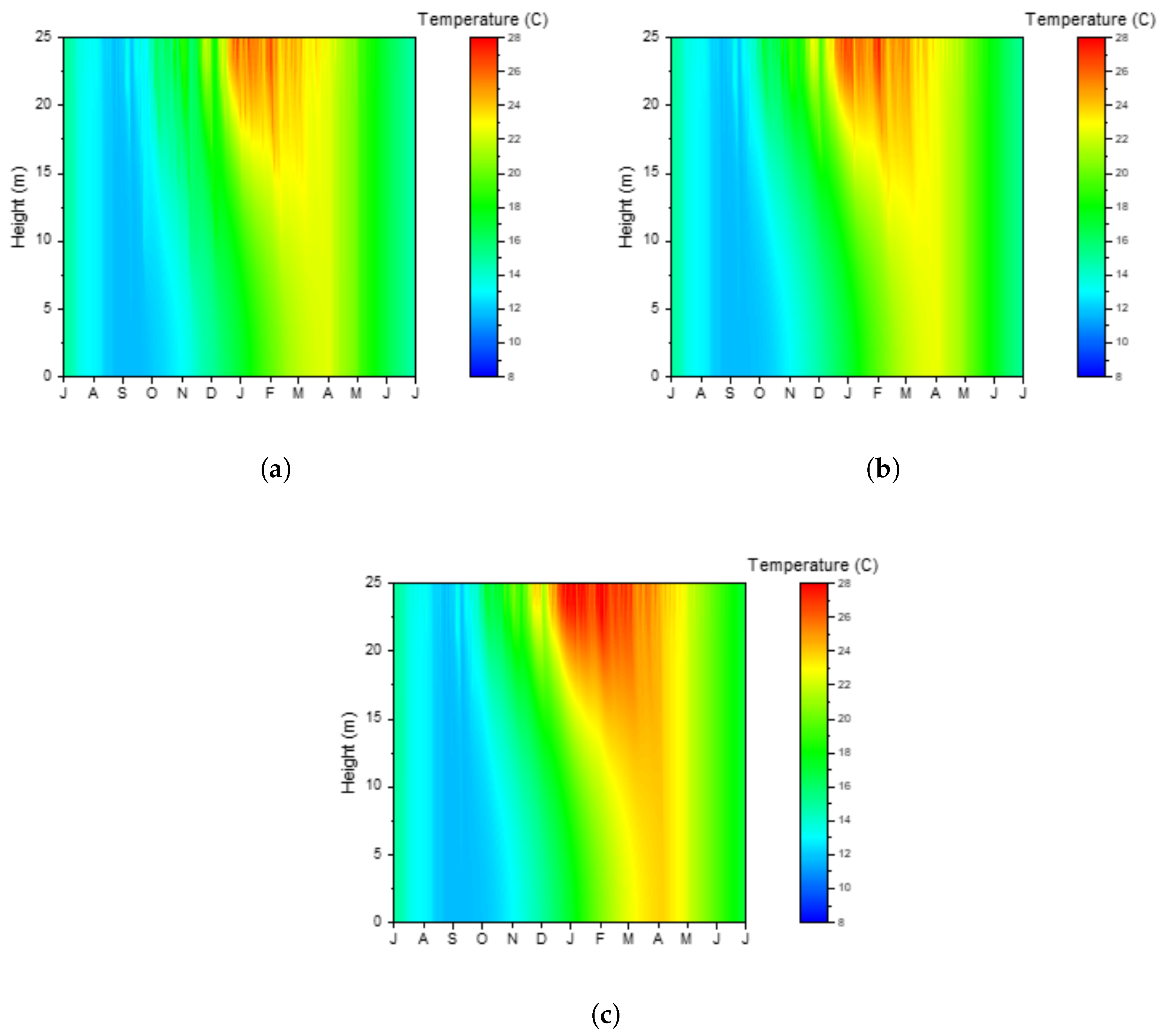
3.1. Temperature and Stratification
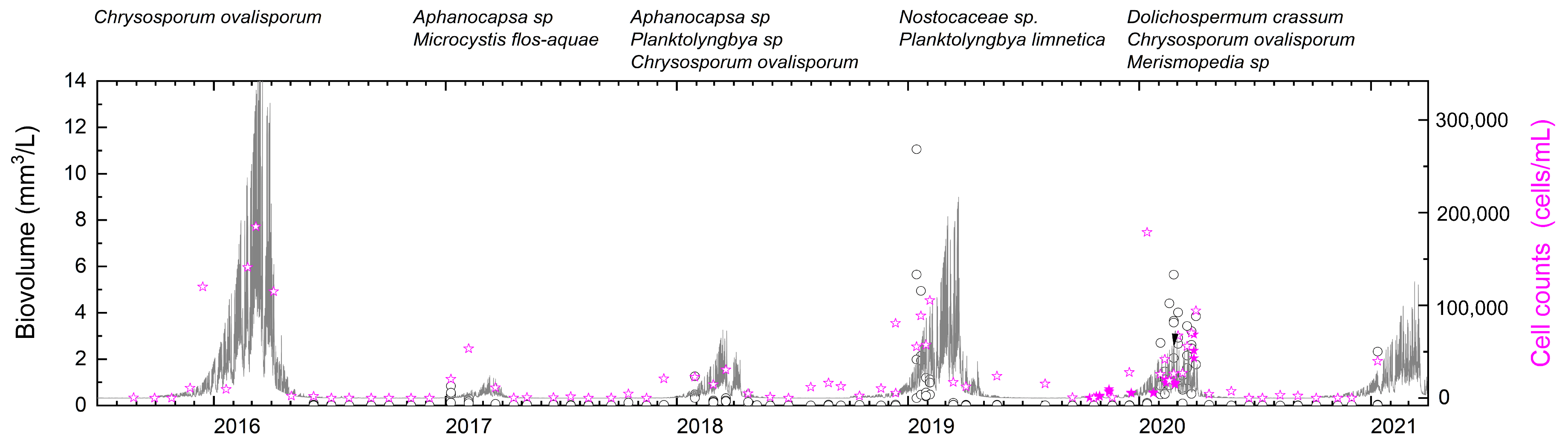
3.2. Blue-Green Algal Growth
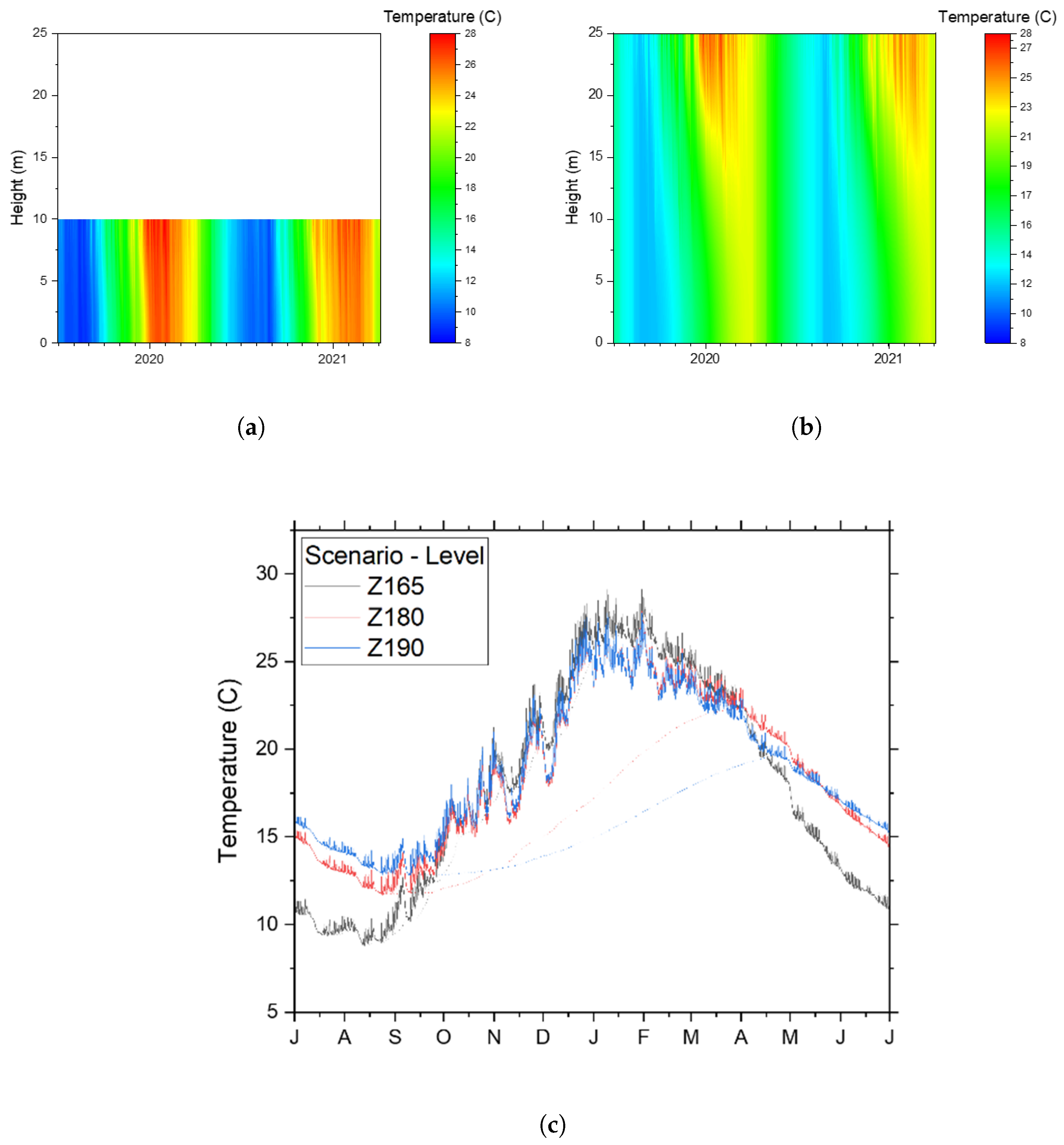
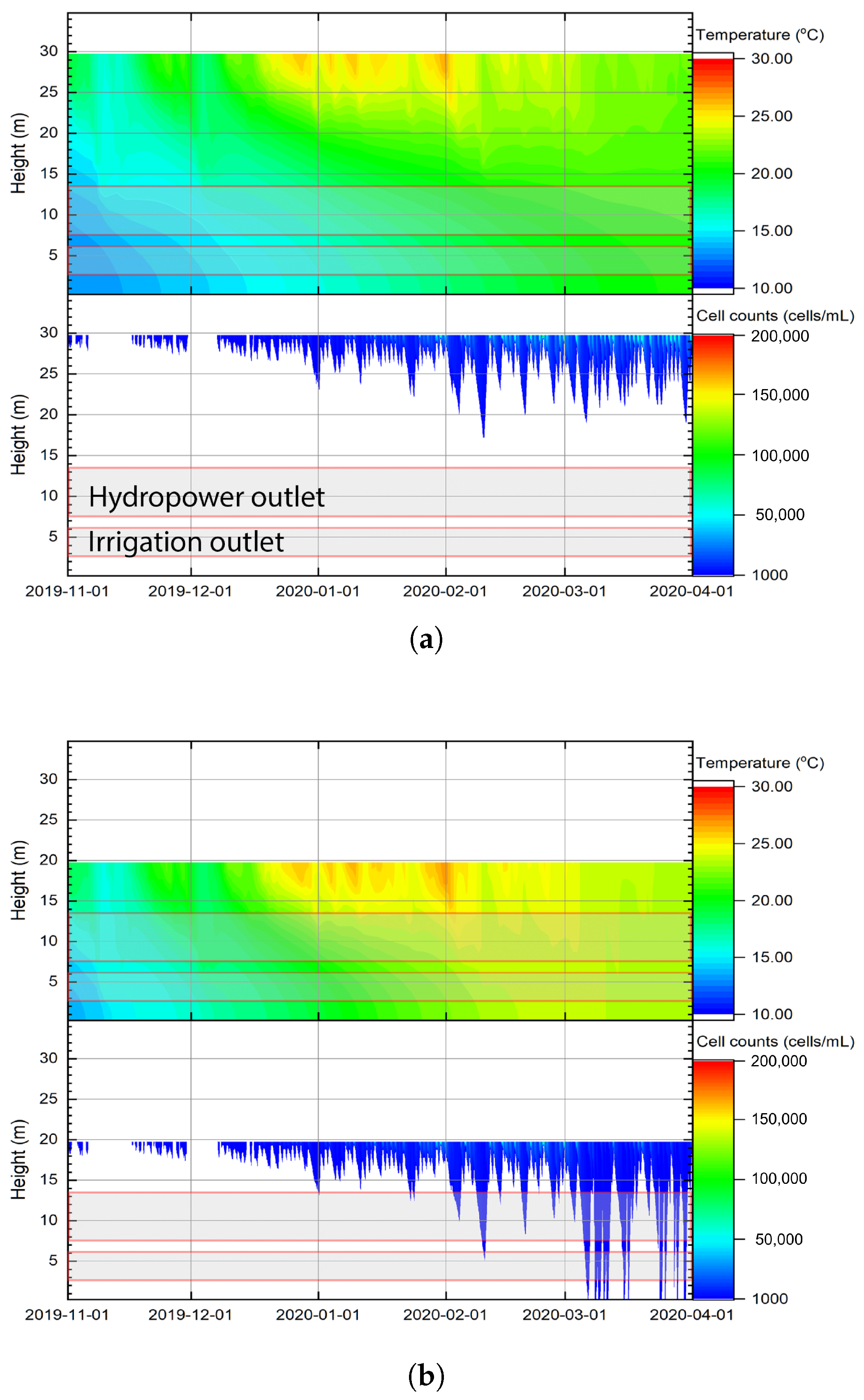
3.3. Stratification and Algal Growth in Relation to Outlets
4. Discussion
5. Conclusions
Author Contributions
Funding
Data Availability Statement
Acknowledgments
Conflicts of Interest
Abbreviations
| ACT | Australian Capital Territory |
| AHD | Australian Height Datum |
| BoM | Bureau of Meteorology |
| BGA | Blue-green algae |
| CSIRO | The Commonwealth Scientific and Industrial Research Organisation |
| GL | Giga Litres |
| LAKEoneD | The one-dimensional lake model |
| MDBA | Murray–Darling Basin Authority |
| NSW | New South Wales |
Appendix A. Stratification and Cyanobacteria Cell Count to Hydropower and Irrigation Outlet at Hume Dam Under Different Water Levels (2015–2021)


References
- Huisman, J.; Codd, G.A.; Paerl, H.W.; Ibelings, B.W.; Verspagen, J.M.H.; Visser, P.M. Cyanobacterial blooms. Nat. Rev. Microbiol. 2018, 16, 471–483. [Google Scholar] [CrossRef] [PubMed]
- Mishra, S.; Stumpf, R.P.; Schaeffer, B.A.; Werdell, P.J.; Loftin, K.A.; Meredith, A. Measurement of Cyanobacterial Bloom Magnitude using Satellite Remote Sensing. Sci. Rep. 2019, 9, 18310. [Google Scholar]
- Baker, P.; Humpage, A. Toxicity associated with commonly occurring cyanobacteria in surface waters of the Murray-Darling Basin, Australia. Aust. J. Mar. Freshw. Res. 1994, 45, 773–786. [Google Scholar]
- van Apeldoorn, M.; van Egmond, H.; Speijers, G.; Bakker, G. Toxins of cyanobacteria. Mol. Nutr. Food Res. 2007, 51, 7–60. [Google Scholar]
- Hilborn, E.D.; Beasley, V.R. One Health and Cyanobacteria in Freshwater Systems: Animal Illnesses and Deaths Are Sentinel Events for Human Health Risks. Toxins 2015, 7, 1374–1395. [Google Scholar] [CrossRef]
- Rastogi, R.P.; Madamwar, D.; Incharoensakdi, A. Bloom Dynamics of Cyanobacteria and Their Toxins: Environmental Health Impacts and Mitigation Strategies. Front. Microbiol. 2015, 6, 1254. [Google Scholar]
- Gallina, N.; Beniston, M.; Jacquet, S. Estimating future cyanobacterial occurrence and importance in lakes: A case study with Planktothrix rubescens in Lake Geneva. Aquat. Sci. 2017, 79, 249–263. [Google Scholar] [CrossRef]
- Ho, J.C.; Michalak, A.M.; Pahlevan, N. Widespread global increase in intense lake phytoplankton blooms since the 1980s. Nature 2019, 517, 667–670. [Google Scholar] [CrossRef]
- Huang, J.; Zhang, Y.; Arhonditsis, G.; Gao, J.; Chen, Q.; Peng, J. The magnitude and drivers of harmful algal blooms in China’s lakes and reservoirs: A national-scale characterization. Water Res. 2020, 181, 115902. [Google Scholar]
- Moreira, C.; Vasconcelos, V.; Antunes, A. Cyanobacterial Blooms: Current Knowledge and New Perspectives. Earth 2022, 3, 127–135. [Google Scholar] [CrossRef]
- O’Neil, J.; Davis, T.; Burford, M.; Gobler, C. The rise of harmful cyanobacteria blooms: The potential roles of eutrophication and climate change. Harmful Algae 2012, 14, 313–334. [Google Scholar]
- Elliott, J.A. Is the future blue-green? A review of the current model predictions of how climate change could affect pelagic freshwater cyanobacteria. Water Res. 2012, 46, 1364–1371. [Google Scholar] [PubMed]
- Paerl, H.W.; Paul, V.J. Climate change: Links to global expansion of harmful cyanobacteria. Water Res. 2012, 46, 1349–1363. [Google Scholar] [PubMed]
- Gobler, C.J. Climate Change and Harmful Algal Blooms: Insights and perspective. Harmful Algae 2020, 91, 101731. [Google Scholar]
- Steffensen, D.; Burch, M.; Nicholson, B.; Drikas, M.; Baker, P. Management of toxic blue–green algae (cyanobacteria) in Australia. Environ. Toxicol. 1999, 14, 183–195. [Google Scholar]
- Haskins, G.; Davey, G. River Murray in Relation to Albury-Wodonga; Gutteridge Haskins & Davey for the Cities Commission: Melbourne, Australia, 1974. [Google Scholar]
- Walker, K.F.; Hillman, T.J. Limnological Survey of the River Murray in Relation to Albury-Wodonga; Albury-Wodonga Development Corporation: Albury, Australia; Gutteridge Haskins and Davey: Sydney, Australia, 1977. [Google Scholar]
- Walker, K.F.; Hillman, T.J. Phosphorus and nitrogen loads in waters associated with the River Murray near Albury-Wodonga, and their effects on phytoplankton populations. Aust. J. Mar. Freshw. Res. 1982, 33, 223–243. [Google Scholar]
- Sullivan, C.; Saunders, J.; Welsh, D. Phytoplankton of the River Murray, 1980–1985; Murray-Darling Basin Commission: Canberra, Australia, 1988. [Google Scholar]
- Water ECOscience. MDBC Water Quality Review Stage 2—Data Analysis; Technical Report 653; Murray-Darling Basin Commission: Canberra, Australia, 2002. [Google Scholar]
- Joehnk, K.; Malthus, T.; Biswas, T. Harmful Algal Blooms Prediction Workshop Proceedings; Technical Report; CSIRO Land and Water: Canberra, Australia, 2019. [Google Scholar]
- Baldwin, D.S.; Wilson, J.; Gigney, H.; Boulding, A. Influence of extreme drawdown on water quality downstream of a large water storage reservoir. River Res. Appl. 2010, 26, 194–206. [Google Scholar]
- Bowling, L.C.; Merrick, C.; Swann, J.; Green, D.; Smith, G.; Neilan, B.A. Effects of hydrology and river management on the distribution, abundance and persistence of cyanobacterial blooms in the Murray River, Australia. Harmful Algae 2013, 30, 27–36. [Google Scholar]
- Kraus, E. Modelling and Prediction of the Upper Layers of the Ocean: Proceedings of a NATO Advanced Study Institute; Pergamon Press: Oxford, UK, 1977. [Google Scholar]
- Cheng, B.; Xia, R.; Zhang, Y.; Yang, Z.; Hu, S.; Guo, F.; Ma, S. Characterization and causes analysis for algae blooms in large river system. Sustain. Cities Soc. 2019, 51, 101707. [Google Scholar]
- Callieri, C.; Bertoni, R.; Contesini, M.; Bertoni, F. Lake level fluctuations boost toxic cyanobacterial “oligotrophic blooms”. PLoS ONE 2014, 9, e109526. [Google Scholar]
- Huang, J.; Xu, Q.; Wang, X.; Ji, H.; Quigley, E.J.; Sharbatmaleki, M.; Li, S.; Xi, B.; Sun, B.; Li, C. Effects of hydrological and climatic variables on cyanobacterial blooms in four large shallow lakes fed by the Yangtze River. Environ. Sci. Ecotechnol. 2021, 5, 100069. [Google Scholar]
- Fuentes, E.V.; Petrucio, M.M. Water level decrease and increased water stability promotes phytoplankton growth in a mesotrophic subtropical lake. Mar. Freshw. Res. 2015, 66, 711–718. [Google Scholar]
- Li, Y.; Fang, L.; Cao, G.; Mi, W.; Lei, C.; Zhu, K.; Bi, Y. Reservoir regulation-induced variations in water level impacts cyanobacterial bloom by the changing physiochemical conditions. Water Res. 2024, 259, 121836. [Google Scholar]
- Imberger, J.; Hamblin, P.F. Dynamics of Lakes, Reservoirs, and Cooling Ponds. Annu. Rev. Fluid Mech. 1982, 14, 153–187. [Google Scholar]
- Imberger, J. The diurnal mixed layer. Limnol. Oceanogr. 1985, 30, 737–770. [Google Scholar]
- Janssen, A.; Arhonditsis, G.; Beusen, A.; Bolding, K.; Bruce, L.; Bruggeman, J.; Couture, R.; Downing, A.; Alex Elliott, J.; Frassl, M.; et al. Exploring, exploiting and evolving diversity of aquatic ecosystem models: A community perspective. Aquat. Ecol. 2015, 49, 513–548. [Google Scholar]
- Frassl, M.A.; Abell, J.M.; Botelho, D.A.; Cinque, K.; Gibbes, B.R.; Jöhnk, K.D.; Muraoka, K.; Robson, B.J.; Wolski, M.; Xiao, M.; et al. A short review of contemporary developments in aquatic ecosystem modelling of lakes and reservoirs. Environ. Model. Softw. 2019, 117, 181–187. [Google Scholar]
- Jöhnk, K.D.; Huisman, J.; Sharples, J.; Sommeijer, B.; Visser, P.M.; Stroom, J.M. Summer heatwaves promote blooms of harmful cyanobacteria. Glob. Chang. Biol. 2008, 14, 495–512. [Google Scholar]
- Howitt, J.; Baldwin, D.S.; Hawking, J. A Review of the Existing Studies on Lake Hume and Its Catchment; Technical Report; Goulburn Murray Water: Shepparton, Australia, 2005; 123p. [Google Scholar]
- Al-Tebrineh, J.; Merrick, C.; Ryan, D.; Humpage, A.; Bowling, L.; Neilan, B.A. Community Composition, Toxigenicity, and Environmental Conditions during a Cyanobacterial Bloom Occurring along 1,100 Kilometers of the Murray River. Appl. Environ. Microbiol. 2012, 78, 263–272. [Google Scholar]
- Baldwin, D. The Potential Impacts of Climate Change on Water Quality in the Southern Murray–Darling Basin; Technical Report; MDFRC Publication 139/2015; The Murray–Darling Freshwater Research Centre: Canberra, Australia; Murray–Darling Basin Authority: Wodonga, Australia, 2016. [Google Scholar]
- Anthony, W.; Friedrich, J. The uptake of amino acids by the cyanobacterium Planktothrix rubescens is stimulated by light at low irradiances. FEMS Microbiol. Ecol. 2006, 58, 14–22. [Google Scholar]
- Baldwin, D.S.; Gigney, H.; Wilson, J.S.; Watson, G.; Boulding, A.N. Drivers of water quality in a large water storage reservoir during a period of extreme drawdown. Water Res. 2008, 42, 4711–4724. [Google Scholar] [CrossRef] [PubMed]
- Sherman, B. Hume Reservoir Temperature Monitoring and Heat Budget—October 2002 to March 2003; Technical Report; CSIRO Land and Water: Canberra, Australia, 2003; 68p. [Google Scholar]
- Fadel, A.; Atoui, A.; Lemaire, B.J.; Vinçon-Leite, B.; Slim, K. Dynamics of the Toxin Cylindrospermopsin and the Cyanobacterium Chrysosporum (Aphanizomenon) ovalisporum in a Mediterranean Eutrophic Reservoir. Toxins 2014, 6, 3041–3057. [Google Scholar] [CrossRef] [PubMed]
- Hadas, O.; Pinkas, R.; Malinsky-rushansky, N.; Shalev-alon, G.; Delphine, E.; Berner, T.; Sukenik, A.; Kaplan, A. Physiological variables determined under laboratory conditions may explain the bloom of Aphanizomenon ovalisporum in Lake Kinneret. Eur. J. Phycol. 2002, 37, 259–267. [Google Scholar] [CrossRef]
- Cirés, S.; Wörmer, L.; Timón, J.; Wiedner, C.; Quesada, A. Cylindrospermopsin production and release by the potentially invasive cyanobacterium Aphanizomenon ovalisporum under temperature and light gradients. Harmful Algae 2011, 10, 668–675. [Google Scholar] [CrossRef]
- Facey, J.A.; Michie, L.E.; King, J.J.; Hitchcock, J.N.; Apte, S.C.; Mitrovic, S.M. Severe cyanobacterial blooms in an Australian lake; causes and factors controlling succession patterns. Harmful Algae 2022, 117, 102284. [Google Scholar] [CrossRef]
- Rinke, K.; Keller, P.S.; Kong, X.; Borchardt, D.; Weitere, M. Ecosystem Services from Inland Waters and Their Aquatic Ecosystems. In Atlas of Ecosystem Services: Drivers, Risks, and Societal Responses; Springer International Publishing: Cham, Switzerland, 2019; pp. 191–195. [Google Scholar]
- Kerimoglu, O.; Rinke, K. Stratification dynamics in a shallow reservoir under different hydro-meteorological scenarios and operational strategies. Water Resour. Res. 2013, 49, 7518–7527. [Google Scholar] [CrossRef]
- Imboden, D.M.; Wüest, A. Mixing Mechanisms in lakes. In Physics and Chemistry of Lakes; Springer: Berlin/Heidelberg, Germany, 1995; pp. 83–138. [Google Scholar]
- Bakker, E.S.; Hilt, S. Impact of water-level fluctuations on cyanobacterial blooms: Options for management. Aquat. Ecol. 2016, 50, 485–498. [Google Scholar] [CrossRef]
- Paerl, H.; Huisman, J. Blooms Like It Hot. Science 2008, 320, 57–58. [Google Scholar] [CrossRef]
- Joehnk, K.; Anstee, J.; Ford, P.; Botha, H.; Sherman, B. Lake Hume Blue-Green Algal Risk Minimisation; Technical Report; Prepared for the Murray Darling Basin Authority; CSIRO Land and Water: Canberra, Australia, 2018; 80p. [Google Scholar]
- Joehnk, K.; Biswas, T.; Anstee, J.; Ford, P.; Botha, H.; Drayson, N.; Kerrisk, G.; Mclnerney, P. Lake Hume Blue Green Algae Monitoring and Forecasting; Technical Report; Prepared for the Murray Darling Basin Authority; CSIRO Land and Water: Canberra, Australia, 2021; 64p. [Google Scholar]
- Murray-Darling Basin Commission. Design and Operation of Hume Dam. 2024. Available online: https://www.mdba.gov.au/water-management/infrastructure/hume-dam (accessed on 10 September 2024).
- Biswas, T.K.; Karim, F.; Kumar, A.; Wilkinson, S.; Guerschman, J.; Rees, G.; McInerney, P.; Zampatti, B.; Sullivan, A.; Nyman, P.; et al. 2019–2020 Bushfire impacts on sediment and contaminant transport following rainfall in the Upper Murray River catchment. Integr. Environ. Assess. Manag. 2021, 17, 1203–1214. [Google Scholar] [CrossRef]
- Joehnk, K. 1D Hydrodynamische Modelle in der Limnophysik—Turbulenz, Meromixis, Sauerstoff. Ph.D. Thesis, Technical University of Darmstadt, Darmstadt, Germany, 2000. [Google Scholar]
- Joehnk, K.; Umlauf, L. Modelling the metalimnetic oxygen minimum in a medium sized alpine lake. Ecol. Model. 2001, 136, 67–80. [Google Scholar] [CrossRef]
- Hutter, K.; Jöhnk, K. Continuum Methods of Physical Modeling—Continuum Mechanics, Dimensional Analysis, Turbulence; Springer: Berlin/Heidelberg, Germany, 2004. [Google Scholar]
- Rodi, W.; International Association for Hydraulic Research. Turbulence Models and Their Application in Hydraulics: A State-of-the Art Review; A.A. Balkema: Rotterdam, The Netherlands, 1993. [Google Scholar]
- Samal, N.R.; Mazumdar, A.; Jöhnk, K.D.; Peeters, F. Assessment of ecosystem health of tropical shallow waterbodies in eastern India using turbulence model. Aquat. Ecosyst. Health Manag. 2009, 12, 215–225. [Google Scholar] [CrossRef]
- Stepanenko, V.M.; Martynov, A.; Jöhnk, K.D.; Subin, Z.M.; Perroud, M.; Fang, X.; Beyrich, F.; Mironov, D.; Goyette, S. A one-dimensional model intercomparison study of thermal regime of a shallow, turbid midlatitude lake. Geosci. Model Dev. 2013, 6, 1337–1352. [Google Scholar] [CrossRef]
- Stepanenko, V.; Jöhnk, K.D.; Machulskaya, E.; Perroud, M.; Subin, Z.; Nordbo, A.; Mammarella, I.; Mironov, D. Simulation of surface energy fluxes and stratification of a small boreal lake by a set of one-dimensional models. Tellus A Dyn. Meteorol. Oceanogr. 2014, 66, 21389. [Google Scholar] [CrossRef]
- Thiery, W.; Stepanenko, V.M.; Fang, X.; Jöhnk, K.D.; Li, Z.; Martynov, A.; Perroud, M.; Subin, Z.M.; Darchambeau, F.; Mironov, D.; et al. LakeMIP Kivu: Evaluating the representation of a large, deep tropical lake by a set of one-dimensional lake models. Tellus A Dyn. Meteorol. Oceanogr. 2014, 66, 21390. [Google Scholar] [CrossRef]
- Huisman, J.; van Oostveen, P.; Weissing, F. Species Dynamics in Phytoplankton Blooms: Incomplete Mixing and Competition for Light. Am. Nat. 1999, 154, 46–68. [Google Scholar] [CrossRef]
- Huisman, J.; Sommeijer, B. Population dynamics of sinking phytoplankton in light-limited environments: Simulation techniques and critical parameters. J. Sea Res. 2002, 48, 83–96. [Google Scholar] [CrossRef]
- Mehnert, G.; Leunert, F.; Cirés, S.; Jöhnk, K.D.; Rücker, J.; Nixdorf, B.; Wiedner, C. Competitiveness of invasive and native cyanobacteria from temperate freshwaters under various light and temperature conditions. J. Plankton Res. 2010, 32, 1009–1021. [Google Scholar] [CrossRef]
- Robson, B.J.; Hamilton, D.P. Summer flow event induces a cyanobacterial bloom in a seasonal Western Australian estuary. Mar. Freshw. Res. 2003, 54, 139–151. [Google Scholar] [CrossRef]
- Fadel, A.; Sharaf, N.; Siblini, M.; Slim, K.; Kobaissi, A. A simple modelling approach to simulate the effect of different climate scenarios on toxic cyanobacterial bloom in a eutrophic reservoir. Ecohydrol. Hydrobiol. 2019, 19, 359–369. [Google Scholar] [CrossRef]
- Davis, T.W.; Berry, D.L.; Boyer, G.L.; Gobler, C.J. The effects of temperature and nutrients on the growth and dynamics of toxic and non-toxic strains of Microcystis during cyanobacteria blooms. Harmful Algae 2009, 8, 715–725. [Google Scholar] [CrossRef]
- Shimoda, Y.; Arhonditsis, G.B. Phytoplankton functional type modelling: Running before we can walk? A critical evaluation of the current state of knowledge. Ecol. Model. 2016, 320, 29–43. [Google Scholar]
- Jöhnk, K.; Brüggemann, R.; Rücker, J.; Luther, B.; Simon, U.; Nixdorf, B.; Wiedner, C. Modelling life cycle and population dynamics of Nostocales (cyanobacteria). Environ. Model. Softw. 2011, 26, 669–677. [Google Scholar]
- de Oliveira Santos, L.; Guedes, I.A.; Azevedo, S.M.F.d.O.; Pacheco, A.B.F. Occurrence and diversity of viruses associated with cyanobacterial communities in a Brazilian freshwater reservoir. Braz. J. Microbiol. 2021, 52, 773–785. [Google Scholar] [CrossRef] [PubMed]
- Harris, T.D.; Reinl, K.L.; Azarderakhsh, M.; Berger, S.A.; Berman, M.C.; Bizic, M.; Bhattacharya, R.; Burnet, S.H.; Cianci-Gaskill, J.A.; de Senerpont Domis, L.N.; et al. What makes a cyanobacterial bloom disappear? A review of the abiotic and biotic cyanobacterial bloom loss factors. Harmful Algae 2024, 133, 102599. [Google Scholar]
- Ingleton, T.; Kobayashi, T.; Sanderson, B.; Patra, R.; Macinnis-Ng, C.M.O.; Hindmarsh, B.; Bowling, L.C. Investigations of the temporal variation of cyanobacterial and other phytoplanktonic cells at the offtake of a large reservoir, and their survival following passage through it. Hydrobiologia 2008, 603, 221–240. [Google Scholar] [CrossRef]
- Steinberg, C.E.W.; Hartmann, H.M. Planktonic bloom-forming Cyanobacteria and the eutrophication of lakes and rivers. Freshw. Biol. 1988, 20, 279–287. [Google Scholar] [CrossRef]
- Williamson, N.; Kobayashi, T.; Outhet, D.; Bowling, L.C. Survival of cyanobacteria in rivers following their release in water from large headwater reservoirs. Harmful Algae 2018, 75, 1–15. [Google Scholar]
- Otten, T.G.; Crosswell, J.R.; Mackey, S.; Dreher, T.W. Application of molecular tools for microbial source tracking and public health risk assessment of a Microcystis bloom traversing 300 km of the Klamath River. Harmful Algae 2015, 46, 71–81. [Google Scholar]
- Crawford, A.; Holliday, J.; Merrick, C.; Brayan, J.; van Asten, M.; Bowling, L. Use of three monitoring approaches to manage a major Chrysosporum ovalisporum Bloom Murray River, Australia, 2016. Environ. Monit. Assess. 2017, 189, 202. [Google Scholar]


| Station Location | Station | Australian Height Datum | Longitude | Latitude | Instruments Deployed |
|---|---|---|---|---|---|
| Dam Wall | HUME_DAM | 157 m | 360600 | 14702′00 | thermistor-chain, met-station |
| North of the Dam | HUME01 | 157 m | 360505 | 14703′07 | four loggers located at 0.5, 5, 15, and 25 m below surface |
| South of the Dam | HUME09 | 160 m | 360702 | 14702′03 | four loggers located at 0.5, 5, 15, and 25 m below surface |
| Calder Bay | HUME10 | 167 m | 360007 | 14705′04 | two loggers located at 0.5, 15 m below surface |
| Huon | HUME06 | 171 m | 360100 | 1470405 | two loggers located at 0.5 and 15 m below surface |
| Intake | Depth [m AHD] |
|---|---|
| hydropower | 162.535–168.679 |
| Irrigation | 157.710–161.367 |
Disclaimer/Publisher’s Note: The statements, opinions and data contained in all publications are solely those of the individual author(s) and contributor(s) and not of MDPI and/or the editor(s). MDPI and/or the editor(s) disclaim responsibility for any injury to people or property resulting from any ideas, methods, instructions or products referred to in the content. |
© 2025 by the authors. Licensee MDPI, Basel, Switzerland. This article is an open access article distributed under the terms and conditions of the Creative Commons Attribution (CC BY) license (https://creativecommons.org/licenses/by/4.0/).
Share and Cite
Nguyen, D.; Biswas, T.; Anstee, J.; Ford, P.W.; Joehnk, K. Managing Cyanobacteria Blooms in Lake Hume: Abundance Dynamics Across Varying Water Levels. Water 2025, 17, 891. https://doi.org/10.3390/w17060891
Nguyen D, Biswas T, Anstee J, Ford PW, Joehnk K. Managing Cyanobacteria Blooms in Lake Hume: Abundance Dynamics Across Varying Water Levels. Water. 2025; 17(6):891. https://doi.org/10.3390/w17060891
Chicago/Turabian StyleNguyen, Duy, Tapas Biswas, Janet Anstee, Phillip W. Ford, and Klaus Joehnk. 2025. "Managing Cyanobacteria Blooms in Lake Hume: Abundance Dynamics Across Varying Water Levels" Water 17, no. 6: 891. https://doi.org/10.3390/w17060891
APA StyleNguyen, D., Biswas, T., Anstee, J., Ford, P. W., & Joehnk, K. (2025). Managing Cyanobacteria Blooms in Lake Hume: Abundance Dynamics Across Varying Water Levels. Water, 17(6), 891. https://doi.org/10.3390/w17060891