High-Temporal-Resolution Modeling of Land Surface Temperature and Groundwater Level Impacts on Shallow Aquifer Thermal Regimes

Abstract

Climate change is recognized to directly and indirectly affect groundwater systems. However, the mechanisms through which climate change influences groundwater temperature (GWT), particularly how seasonal variations mediate these effects, remain incompletely understood. This study utilized high-temporal-resolution (hourly) data by parameterizing groundwater levels (GWLs) and instantaneous temperature gradients to model GWT, establishing the Seasonally Adaptive Thermal Diffusivity Numerical Model (SATDNM). Through scenario analyses, the potential impacts of climate change on GWT were simulated. The results indicate that our model captures seasonal and interannual variations more precisely compared to classical models, revealing the seasonal influence of GWLs and instantaneous temperature gradients on subsurface thermal properties such as advents and wet-season rainfall, as well as long-term surface warming and GWL decline. The key findings include (1) a greater sensitivity to extreme heat during winter, (2) wet-season rainfall potentially stabilizing groundwater temperature, and (3) declining GWLs amplifying GWT fluctuations. By 2100, the projected mean GWT increases under four Shared Socioeconomic Pathway (SSP) scenarios are approximately 0.51 °C (SSP1-2.6), 1.25 °C (SSP2-4.5), 2.19 °C (SSP3-7.0), and 2.87 °C (SSP5-8.5). Under four scenarios of annual GWL decline rates, GWT fluctuations increased by approximately 0.094 °C (0.01 m/year), 0.27 °C (0.02 m/year), 0.44 °C (0.03 m/year), and 0.67 °C (0.04 m/year), respectively. These findings enhance the mechanistic understanding of climate–groundwater thermal interactions and provide new insights for adaptive groundwater management under climate change.

1. Introduction

As the world’s largest reservoir of liquid freshwater, groundwater systems play a critical role in sustaining ecosystems and ensuring human adaptation to extreme and unexpected global environmental changes [1]. Especially in recent years, groundwater resources have been severely damaged in the face of rapid population growth and climate change [2]. The dual challenge of continued land surface temperature (LST) increases and declining GWLs has led to increasingly complex thermal response mechanisms in groundwater systems. Surface warming significantly affects shallow GWTs through thermal diffusion processes [3]. Benz et al. [4] conservatively estimate that under the medium emission scenario, the average temperature of groundwater will increase by 2.1 °C from the year 2000 to 2100. A thermodynamic imbalance in a groundwater system not only alters its physical state but may also trigger a cascading response of migratory transformations in the groundwater’s chemical components and microbial community structure. Studies have shown that higher GWTs accelerate mineral weathering, leading to higher concentrations of elements such as manganese and other drinking water-related elements [5,6]. Microbial respiration and growth rates, mineral solubility, and solute diffusion rates in groundwater all exhibit significant temperature dependence [7,8,9]. In coastal unconfined aquifers, microbial activity and chemical reactivity are strongly influenced by temperature, which can vary spatially and temporally with changes in GWT [10]. It is worth noting that subsurface heat transfer does not appear to take into account changes in subsurface thermal properties due to changes in GWLs. However, there are significant thermal property differences between saturated and unsaturated aquifers due to their different void water contents [11]. Meanwhile, for shallow temperatures, vapor movement in the vadose zone is again an important factor affecting subsurface heat transfer [12,13]. For modeling fine temperatures, it is important to understand how changes in these influences affect thermal properties. It is also unknown whether these factors will indirectly affect GWTs under climate change.

However, research examining the relationship between other influencing factors and GWT under climate change is limited, and knowledge gaps remain. Previous studies investigating the impacts of climate change on groundwater systems have focused mainly on groundwater resources and long-term GWT changes, largely ignoring seasonal subsurface thermal responses, especially the indirect impacts of climate change products on groundwater, such as declining GWLs and the impacts of extreme rainfall events on groundwater [14,15]. Secondly, most studies considering shallow subsurface heat transport have used constant thermal parameters to model interannual temperature variations [16,17]. However, subsurface thermal property parameters usually vary with seasonal variations, and subsurface thermal properties vary under different external conditions. Instantaneous vertical water fluxes in the subsurface can modify the subsurface temperature field and be used to quantify surface water and groundwater interactions [18]. Subsurface thermal conductivity is affected by its moisture content, which in turn is affected by the GWL [19,20,21]. Seasonal and spatial variations in GWLs can lead to significant differences in thermal conductivity and diffusivity. At the same time, temperature gradients affect the thermal conductivity of soil [22,23]. These studies typically either discuss instantaneous hydrothermal groundwater movement and effects in terms of constant thermal properties or use constant thermal properties to discuss the direct effects of global average temperature increases on groundwater systems on an interannual scale. To the best of our knowledge, no one has examined the effects of intra-annual seasonal variations in thermal properties on the groundwater system and the possible effects of products under climate change on the groundwater system.

The aim of this study is to focus on the following: (1) the higher-temporal-resolution numerical modeling of GWT; (2) how seasonal variations in GWLs and surface temperature affect GWT; and (3) possible future changes in GWT in the context of intensifying climate change and their possible impacts.

2. Material and Methods

2.1. Classical One-Dimensional Heat Transfer Equation

Vertical one-dimensional conductive heat transfer in an isotropic medium that can be described as follows [24]:

$${\displaystyle \frac{\partial T}{\partial t}}=K_r{\displaystyle \frac{{\partial }^{2}T}{\partial z^2}}$$

(1)

where $K_r$ is the thermal diffusivity (m² s⁻¹), $T$ is the temperature (°C), $Z$ is the depth from the surface (m), and $t$ is time (s). Equation (1) is only applicable if the following assumptions are made: (1) the thermophysical properties of the medium and fluid are constant in time and at each layer and (2) heat is transmitted only along the Z axis.

Assume the surface is subject to boundary conditions:

$$T\left(0,t\right)=T_m+A_0\cos ({\displaystyle \frac{2\pi }{p}}t)$$

(2)

where $T\left(0,t\right)$ is a function of time at $Z=0$; we employ the cosine-fitted LST as the boundary condition at $Z=0$. The fitted LST is used here to meet the boundary condition requirements of the classical analytical method. $T_m$ is the mean cosine-fitted LST, and $A_0$ is the amplitude of the cosine-fitted LST. $p$ represents the period, which is one year in Equation (2).

And the obey boundary conditions at infinity can be defined as follows:

$$T\left(\infty ,t\right)-T_m=0$$

(3)

Carslaw et al. [25] gave the following classical analytical solution for the subsurface temperature:

$$T\left(z,t\right)=A_0{e}^{-\sqrt{{\displaystyle \frac{\pi }{K_{r}p}}}z}\cos ({\displaystyle \frac{2\pi }{p}}t-\sqrt{{\displaystyle \frac{\pi }{\alpha p}}}z)$$

(4)

where $T\left(z,t\right)$ is the thermal response of the sediments to the surface boundary conditions at time $t$ and depth $z$; $A_0$ is the amplitude of the LST.

Based on Equation (4), a number of methods for the thermal tracing of surfaces and groundwater can also be derived by including a convective term: methods based on phase lag and amplitude decay models [26,27,28,29], methods based on the frequency domain to estimate vertical water fluxes and effective heat diffusivity in the riverbed [30,31], or methods based on Green’s function approach to deal with solving problems with arbitrary initial and boundary conditions [32].

In the classical approach, we typically use reverse modeling to infer the thermal diffusivity from temperature data and then derive the temperature distribution along the entire vertical direction. This method, based on the analytical derivation of physical equations, relies on back-calculating thermal diffusivity from the observed temperature variations rather than directly estimating it from actual parameters. Constrained by the cosine boundary conditions of the analytical solution, the classical method can only use a fixed thermal diffusivity parameter. Moreover, this method does not allow for the estimation of thermal diffusivity from the parameters themselves, which prevents us from parameterizing other influencing factors.

2.2. Estimation of Seasonally Varying Thermal Diffusivity

In this section, we present a method for estimating seasonally varying thermal diffusivity, where the influencing factors include groundwater level and transient temperature gradient.

Thermal conductivity ($\lambda$) is a unique soil thermal property that governs heat transfer in soils. A correct estimation of soil thermal conductivity and clarification of thermal conductivity variations over the course of a year are important for the accurate prediction of subsurface temperature changes, although variations in soil thermal conductivity are difficult to predict because of a number of factors affecting soil thermal conductivity, such as porosity, saturation degree, quartz content, sand content, and other factors such as grain shape, packing geometry, and grain and pore size distributions [33,34,35]. Many models have been developed to predict the thermal conductivity of soils [36,37,38]. However, there is no specific solution to understanding the relative seasonal changes in soil thermal conductivity.

The methods described in Section 2.1 share a common limitation: thermal diffusivity is assumed to be constant in their formulations. However, over extended simulation periods, variations in rainfall and air temperature induce dynamic changes in soil temperature and moisture content, thereby altering thermal diffusivity. Consequently, while these models effectively capture diurnal-scale temperature fluctuations, they are rarely applicable to interannual thermal predictions. The temperature-dependent thermal diffusivity $K_r$ is defined as follows in Equation (5):

$$K_r={\displaystyle \frac{\lambda }{C}}+\beta {\left({\displaystyle \frac{C_w}{C}}q\right)}^m$$

(5)

where $\lambda$ is the baseline thermal conductivity of the saturated medium (W·m⁻¹·K⁻¹); $\beta$ is the thermal dispersivity; and $m$ is an empirical coefficient. $C$ and $C_w$ are the volumetric heat capacity of the saturated sediment and water (J⋅m⁻³⋅K⁻¹), and $q$ is the vertical Darcy flux (m s⁻¹). Generally, at lower flow rates, we ignore the second term of Equation (5) [39].

We know that the composition, particle size, porosity, etc., of the soil at a given site is difficult to change in a short period of time. In addition to these, the dominant factors controlling thermal conductivity are soil moisture content and temperature. The seasonally varying thermal conductivity can be expressed as a function of time as follows:

$$\lambda \left(t\right)={\lambda }_w\left(t\right)+{\lambda }_T\left(t\right)$$

(6)

Here, ${\lambda }_w\left(t\right)$ represents the influence of seasonal GWL changes on the thermal conductivity, and ${\lambda }_T\left(t\right)$ represents the influence of the instantaneous temperature gradient on the thermal conductivity.

The GWL represents the interface between saturated and unsaturated aquifers, which directly affects the water content in the pore space, and the water content change is often considered to be the main factor affecting soil thermal conductivity [40]. Therefore, we assume that the unsaturated thermal conductivity ${\lambda }_{us}$ and the saturated thermal conductivity ${\lambda }_s$, which are affected by the water content, remain constant and that the change at a given time is controlled only by the GWL. In other words, the thermal conductivity change in the whole aquifer at a given time is controlled only by the GWL, as in Equation (7).

$${\lambda }_w(t)=({\displaystyle \frac{d\left(t\right)}{d_{sensor}}}{\lambda }_{us}+(1-{\displaystyle \frac{d\left(t\right)}{d_{sensor}}}){\lambda }_s)+(-k{\displaystyle \frac{\partial d}{\partial t}}\left({\lambda }_s-{\lambda }_{us}\right))$$

(7)

where $d\left(t\right)$ is the groundwater depth (m) at time $t$ (decreasing as the GWL rises); $d_{sensor}$ is the depth at the monitoring location (m); ${\lambda }_{us}$ and ${\lambda }_s$ are the effective thermal conductivity of unsaturated and saturated aquifers (W·m⁻¹·K⁻¹), and in general, ${\lambda }_{us}<{\lambda }_s$, where increasing water content increases thermal conductivity; $k$ is a dimensionless coefficient measuring the intensity of the thermal conductivity change due to changes in the GWL; and ${\displaystyle \frac{\partial d}{\partial t}}$ is the groundwater depth change rate (m h⁻¹) at time $t$ (negative for rising GWL). The first term in this Equation quantifies the instantaneous effective thermal conductivity properties, while the second term evaluates the vertical heat transfer modulation induced by groundwater flow dynamics through GWL variations. Specifically, a positive second term during GWL rise indicates a downward vertical flow, which enhances aquifer thermal conductivity through advective heat transport.

The soil temperature gradient is an important factor affecting the migration of soil water, air, and heat. The transfer of steam, driven by changes in temperature gradients, is crucial for the movement of mass and energy within soil [41,42]. Mandavi et al. [13] conducted experiments on heat and water transport in soil columns with osmotic gradients and discovered that approximately 96% of the steam transfer was attributed to temperature gradients. The upward vapor transport within soil exerts a measurable perturbation on heat flux distribution. To quantify the seasonal variations in effective soil thermal conductivity arising from evolving temperature gradients, we characterize the thermal gradient using the differential between the LST and average GWT. Furthermore, the influence of vapor transport on thermal conductivity is parameterized as a linear functional dependence relative to this temperature gradient, as follows:

$${\lambda }_T\left(t\right)=m\left({\overline{T_{GWT}}-T}_{LST}\left(t\right)\right)$$

(8)

where $\overline{T_{GWT}}$ represents the average GWT; $T_{LST}\left(t\right)$ represents the land surface temperature (LST) at time $t$; and $m$ is a dimensionless positive coefficient that measures the extent to which the temperature difference affects the effective thermal conductivity. When ${\overline{T_{GWT}}>T}_{LST}$, ${\lambda }_T\left(t\right)$ is positive. In this scenario, the temperature difference enhances the effective thermal conductivity, as the upward thermal gradient in the subsurface facilitates upward vapor transport, promoting heat transfer. Conversely, when ${\overline{T_{GWT}}<T}_{LST}$, ${\lambda }_T\left(t\right)$ becomes negative, and this difference reduces the effective thermal conductivity because the vapor movement opposes the heat transfer direction, thereby impeding heat flow.

The heat capacity is also measured by means of the GWL:

$$C={\displaystyle \frac{d\left(t\right)}{d_{sensor}}}{C}_s+(1-{\displaystyle \frac{d\left(t\right)}{d_{sensor}}})(p{\mathrm{C}}_{\mathrm{w}}+\left(1-p\right){\mathrm{C}}_{\mathrm{s}})$$

(9)

where $C_s$ represents the volumetric heat capacity of the solids; ${\mathrm{C}}_{\mathrm{w}}$ represents the volumetric heat capacity of water; and $p$ represents the porosity of the porous medium.

The final effective thermal diffusivity seasonal variation with time is determined in Equation (10):

$$K_r\left(\mathrm{t}\right)={\displaystyle \frac{(\frac{d\left(t\right)}{d_{sensor}}{\lambda }_{us}+(1-\frac{d\left(t\right)}{d_{sensor}}){\lambda }_s)+k\frac{\partial d}{\partial t}\left({\lambda }_{us}-{\lambda }_s\right)+m\left({\overline{T_{GWT}}-T}_{LST}(t)\right)}{\frac{d\left(t\right)}{d_{sensor}}{C}_s+(1-\frac{d\left(t\right)}{d_{sensor}})(p{\mathrm{C}}_{\mathrm{w}}+\left(1-p\right){\mathrm{C}}_{\mathrm{s}})}}$$

(10)

2.3. Differences in the Direction of Heat Transfer Leads to Differential Rises and Declines in GWT

Solar radiation, which originates from the sun and reaches the Earth’s surface, serves as the main heat source for both the Earth’s surface and its atmosphere. Upon striking the Earth’s surface, this radiation is absorbed by various materials such as soil and rocks. The absorption of solar radiation leads to an increase in the temperature of the Earth’s surface [43]. This implies that solar radiative forcing constitutes a dominant driver of terrestrial surface temperature variations, with incident solar energy being the principal contributor to surface warming regardless of seasonal variations between summer and winter periods [44]. In summer, GWT is lower than surface temperature, and the subsurface thermal regime is primarily governed by unidirectional downward conductive heat transfer from the surface, with negligible direct radiative forcing from solar energy, and varies synchronously with surface temperature changes. In winter, when GWT exceeds surface temperature, the thermal regime becomes complex. Due to the subsurface temperature being higher than the surface temperature, heat transfers upward toward the surface. However, concurrent solar radiative forcing directly impacts surface temperature. This results in two distinct heat transfer modes governing GWT dynamics during its warming and cooling phases.

We demonstrate this with hourly data on GWT. Figure 1 calculates the GWT change rate. A clear observation reveals that GWT derivatives exhibit significant fluctuations during the cooling phase, contrasting sharply with the extreme stability observed during the warming phase, as shown by the green curve in Figure 1a. During the warming phase, the derivatives are consistently positive (>0), as shown in Figure 1b, indicating a stable temperature increase. Conversely, in the cooling phase, the derivatives do not remain entirely negative (<0), as depicted in Figure 1c, with temperature exhibiting a diurnal-scale oscillatory decline. Notably, the maximum fluctuation amplitude during the cooling phase exceeds that of the warming phase by an order of magnitude (10×).

To further substantiate the distinction between the two heat transfer modes, we compared the temperature variation rate (with diurnal fluctuations removed) against the groundwater depth variation rate, as illustrated in Figure 2. Our findings revealed differing impacts of groundwater depth dynamics on temperature changes during the warming and cooling phases. During the warming phase, variations in groundwater depth do not alter the temperature derivative, which continues to follow diurnal fluctuation patterns. Only abrupt changes can transiently affect the magnitude of these diurnal oscillations, and it quickly recovers. In contrast, during the cooling phase, the temperature derivative demonstrates significantly heightened sensitivity to water level fluctuations, exhibiting a somewhat linear relationship. These two phases are governed by fundamentally distinct dominant mechanisms. Consequently, we conceptualize the rise (warming)-phase and decline (cooling)-phase heat transfer processes as two distinct modes, each with separate parameters. The parameters governing thermal conductivity and GWL effects are segregated by the warming and cooling phases. We regard the surface temperature being higher than the GWT as the warming phase, and lower than the GWT as the cooling phase.

2.4. Seasonally Adaptive Thermal Diffusivity Numerical Model (SATDNM)

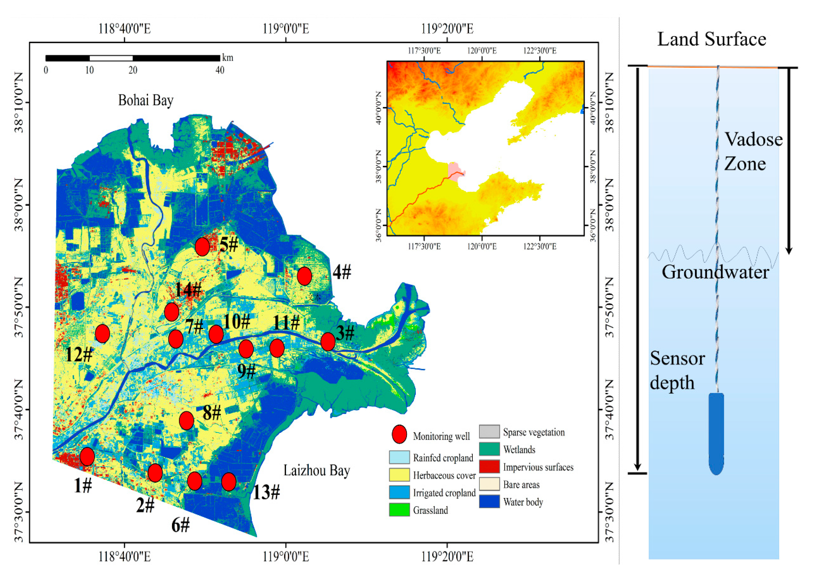
Following the classic 1D unsteady heat conduction equation (Section 2.1), we formulate the finite difference approximation of the temporal derivative at spatial node $i$ as follows in Equation (11). Here, we denote $T_i$ as the temperature $T_{GWT}$ at the location of the sensor based on the measured real data.

$${\left.{\displaystyle \frac{\partial T}{\partial t}}\right|}_i\approx {\displaystyle \frac{T_i^{n+1}-T_i^n}{∆t}}={\displaystyle \frac{T_{GWT}^{n+1}-T_{GWT}^n}{∆t}}$$

(11)

The superscript $n$ indicates the time-dependent nature of $T$, and the time derivative is represented by the temperature difference between the new time step $(n+1)$ and the previous time step $\left(n\right)$. Here, hourly data are used, so $∆t$ is 1 h.

In the spatial direction, we express the second-order derivatives of the space at $i$ using the central difference approximation, as shown in Equation (12).

$$K_r\left(n\right){\left.{\displaystyle \frac{{\partial }^{2}T}{\partial x^2}}\right|}_i\approx K_r\left(n\right){\displaystyle \frac{T_{i+1}^n-2T_i^n+T_{i-1}^n}{{\left(∆x\right)}^2}}=K_r\left(n-{∆t}_{lag}\right){\displaystyle \frac{T_{LST}^{n-{∆t}_{lag}}-2T_{GWT}^{n-{∆t}_{lag}}+T_{\infty }^{n-{∆t}_{lag}}}{d_{sensor}^2}}$$

(12)

The spatial nodes $i+1$, $i$, and $i-1$ are, respectively, assigned to $T_{LST}$ (land surface temperature), $T_{GWT}$ (GWT at sensor depth), and $T_{\infty }$. Here, $T_{\infty }$ represents the temperature at twice the sensor depth, where thermal fluctuations are sufficiently attenuated to approximate the far-field boundary condition.

In calculating spatial gradients, we assume that temperature waves propagate linearly and maintain mutual independence (linear wave propagation) at each timestep. This implies the second derivative of temperature remains essentially invariant during propagation, with only the amplitude undergoing exponential decay as a function of the propagation distance. We approximate the second derivative of temperature at the sensor location using $T_{LST}$, $T_{GWT}$, and $T_{\infty }$. This approximation introduces a time lag ${∆t}_{lag}$ compared to the actual temperature derivative. When the surface temperature changes, the calculated second derivative immediately responds, but in reality, changes in surface temperature do not instantaneously alter the second derivative at the probe depth. Therefore, we must account for the delayed response of the second derivative caused by surface temperature variations. Assuming a sudden increase or decrease in the surface temperature with the change in moment $n$, the time required for this disturbance to reach the probe depth can be evaluated using the Fourier number, which in finite-difference methods is expressed in its discrete form as follows:

$$Fo={\displaystyle \frac{K_r\left(n\right){∆t}_{lag}}{d_{sensor}^2}}$$

(13)

The time when the disturbance of the surface temperature wave reaches the depth where the sensor is located is expressed as

$${∆t}_{lag}={\displaystyle \frac{Fo{d}_{sensor}^2}{K_r\left(n\right)}}$$

(14)

Here, we take $Fo$ to be between 0.2 and 0.32. Generally speaking, in numerical calculations, when the Fourier number is greater than 0.2, the deviation between the calculation result obtained by omitting the second and subsequent terms of the infinite series and the result calculated by the complete series is less than 1%. Therefore, we consider that the disturbance reaches the probe position when the Fourier number is greater than 0.2. The specific value depends on the fitting situation. Here, the time for the disturbance to reach the depth where the sensor is located is controlled by the thermal diffusivity $K_r\left(n\right)$, that is, the disturbance time at each moment is different.

Finally, the one-dimensional heat conduction equation based on the finite difference method can be derived.

$${\displaystyle \frac{T_{GWT}^{n+1}-T_{GWT}^n}{∆t}}=K_r\left(n-{∆t}_{lag}\right){\displaystyle \frac{T_{LST}^{n-{∆t}_{lag}}-2T_{GWT}^{n-{∆t}_{lag}}+T_{\infty }^{n-{∆t}_{lag}}}{d_{sensor}^2}}$$

(15)

The temperature at the sensor at time step $n+1$ can be formulated as

$$\left\{\begin{array}{c}{T}_{GWT}^{n+1}=T_{GWT}^n+{\displaystyle \frac{K_r\left(n-{∆t}_{lag}\right)}{d_{sensor}^2}}∆t\left(T_{LST}^{n-{∆t}_{lag}}-2T_{GWT}^{n-{∆t}_{lag}}+T_{\infty }^{n-{∆t}_{lag}}\right)\\ {∆t}_{lag}={\displaystyle \frac{Fo{d}_{sd}^2}{K_r\left(n\right)}}\end{array}\right.$$

(16)

Here, we utilize the temperature relationship at time step $n-{∆t}_{lag}$ to quantify the increment from $n-{∆t}_{lag}$ to $T_{GWT}^{n+1}$.

Table 1. The model input parameters.

Parameters	Values	Unit
Porosity, $p$	0.5–0.55
Volumetric heat capacity of solid, $C_s$	(1.5–2.5) × 106	J⋅m−3⋅K−1
Volumetric heat capacity of water, $C_w$	4.18 × 106	J⋅m−3⋅K−1
Unsaturated aquifer thermal conductivity (warming), ${\lambda }_{w-us}$	1–2.6	W·m−1·K−1
Saturated aquifer thermal conductivity (warming), ${\lambda }_{w-s}$	1.43–3	W·m−1·K−1
Unsaturated aquifer thermal conductivity (cooling), ${\lambda }_{c-us}$	0.2–1.9	W·m−1·K−1
Saturated aquifer thermal conductivity (cooling), ${\lambda }_{c-s}$	0.35–2.4	W·m−1·K−1
GWL variation coefficient (warming) $k_w$	0–150
GWL variation coefficient (cooling) $k_c$	0–400
Temperature gradient coefficient, $m$	0.025–0.05
Fourier number, $Fo$	0.2–0.32

lists the parameters, their ranges, and units used in the simulation.

2.5. Data Source

The simulation employs groundwater monitoring data from the Yellow River Delta region, utilizing Solinst Levellogger 5 (Solinst Canada Ltd., Georgetown, ON, Canada) devices for real-time continuous monitoring of the GWL and GWT in unconfined aquifers. A total of 14 hourly groundwater monitoring wells were installed in the study area to monitor GWT, groundwater depth, and electrical conductivity. The depth of all wells was approximately 6 m, and the groundwater depth was within 4 m of the surface. The monitoring well sensors were mostly located around 4 m. All monitoring wells were dated between May 2019 and August 2023. Figure 3 is the location map of the study area and monitoring wells.

The land surface temperature (LST) used ERA5 data from the European Center for Medium-Range Weather Forecasts (ECMWF), accessible through the Copernicus Climate Change Service (https://cds.climate.copernicus.eu (accessed on 17 May 2019 to 26 August 2023)), which provides hourly surface temperature data with a spatial resolution of 0.1° × 0.1°. The analysis utilized the Google Earth Engine (GEE) platform to extract time series data of surface temperature pixels at the monitoring well locations.

3. Results

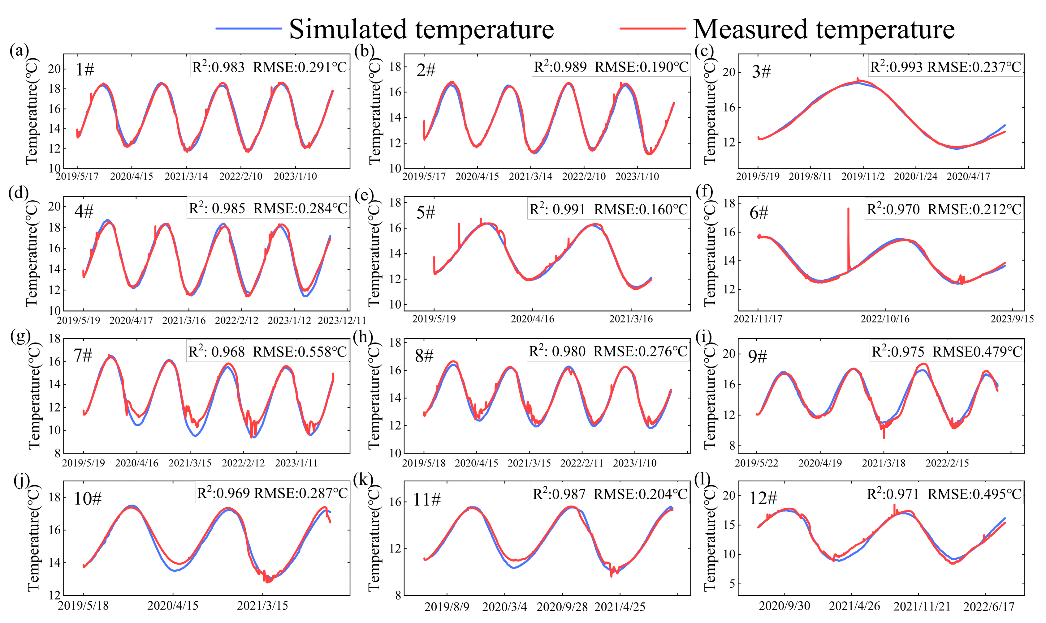
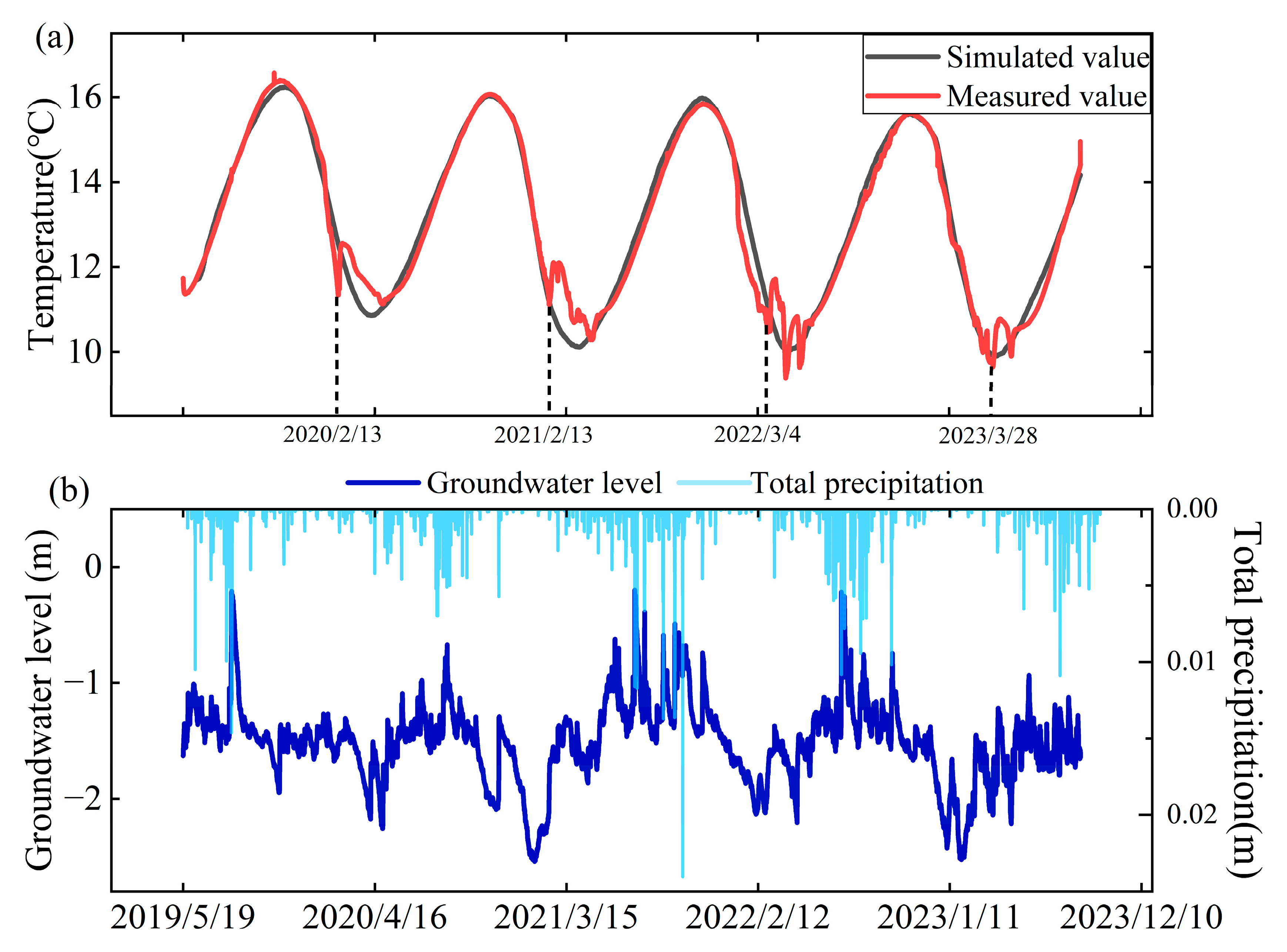
3.1. Model Evaluation

3.1.1. Comparison of SATDNM with Classical Analytical Models

Figure 4 compares the simulated and observed results. For each monitoring well, we assigned initial values $T_{GWT}^0$ and $T_{GWT}^{{∆t}_{lag}}$, then computed the incremental change from $T_{GWT}^{{∆t}_{lag}}$ to $T_{GWT}^{{∆t}_{lag}+1}$ using values at $n=0$. Iterating this process yielded temperature values across all time steps. The results show that all simulations achieved $R^2>0.95$ and a root mean square error $\mathrm{R}\mathrm{M}\mathrm{S}\mathrm{E}<0.5 °\mathrm{C}$. For groundwater systems with minimal external disturbances, the $\mathrm{R}\mathrm{M}\mathrm{S}\mathrm{E}$ could be further reduced to $<0.3 °\mathrm{C}$. The temperature anomalies in some wells are attributed to anthropogenic impacts or extreme precipitation events. Notably, incorporating GWL variations and instantaneous temperature gradients significantly improved the simulation accuracy of sub-seasonal fluctuations and interannual variability in GWT. This demonstrates that GWL dynamics and instantaneous thermal gradients are likely key drivers of seasonal temperature variations in groundwater systems.

Figure 5 compares the analytical solution derived from the heat conduction equation in Section 2.1 with field measurements [25]. Compared to Figure 4, the $R^2$ and $\mathrm{R}\mathrm{M}\mathrm{S}\mathrm{E}$ values in Figure 5 are inferior, and the simulation details are less accurate. In this analytical method, thermal diffusivity is assumed constant throughout the year, with identical upward and downward heat conduction processes. The GWTs follow the cosine form exactly throughout the year, lacking interannual and seasonal variability. However, the field observations revealed asymmetric temperature patterns and interannual fluctuations in coastal shallow aquifers. The classical method exhibited 30 to 60 days discrepancies in predicting minimum temperature, with interannual differences observed at the same monitoring wells. In contrast to the classical analytical approach, the numerical method incorporating seasonal variations in thermal diffusivity aligned more closely with the observed trends. Significant improvements were achieved in capturing the timing of temperature maxima and minima. The numerical model also reasonably simulated the annual variations at individual wells, including interannual changes in peak and trough magnitudes. Under anthropogenic disturbances, the numerical method outperformed the classical approach in replicating realistic patterns. The irregular winter temperature fluctuations (February to May) in Figure 5g–i are attributed to human activities.

3.1.2. Modeling and Testing of Vertical Variation

The downward heat transfer from the surface temperature governs the thermal regime of shallow sediments, with subsurface temperatures exhibiting a temporal lag relative to the surface temperature, and it significantly attenuates fluctuations. As depth increases, both the phase lag and amplitude reduction in the shallow GWT become more pronounced. To validate the model’s performance across varying depths, we analyzed two monitoring wells with adjusted depths. For Well 13# (Figure 6a–c), the initial monitoring depth was 5.0 m. On 24 October 2019, the sensor was raised by 1.671 m to 3.329 m, and was subsequently lowered by 0.45 m to 3.779 m on 27 January 2022. By adjusting the model’s depth parameters, simulated temperatures at 5.0 m, 3.329 m, and 3.779 m showed excellent agreement with field measurements. Deeper layers demonstrated delayed peak/trough timing and reduced amplitude, consistent with theoretical expectations. Similarly, for Well 14# (Figure 6d,e), when the monitoring depth was changed from 4.77 m to 3.689 m on 15 August 2022, the simulated results at both depths closely matched the observations. In contrast to conventional methods that require long-term time-series data at fixed depths to determine thermal diffusivity, our approach dynamically adapts to depth variations while maintaining high accuracy.

Figure 7 presents simulated GWT profiles across depths from 3 m to 6 m at 0.5 m intervals. Figure 7a,c illustrate temperature variations over time, demonstrating the expected variations: as depth increases, the thermal amplitude decreases and phase lag extends. Figure 7b,d show spatial variations in the mean temperature, with 0 m representing the average surface temperature. The model accurately reproduces vertical geothermal gradients under contrasting conditions. For Well 13# (Figure 7b), the mean temperature decreases with depth, reflecting a negative geothermal gradient, while Well 14# (Figure 7d) exhibits the opposite trend, with the mean temperature increasing with depth, indicating a positive geothermal gradient. These results validate the model’s capability to simulate divergent subsurface thermal regimes, capturing both amplitude attenuation and phase delay dynamics across varying depths while maintaining fidelity to site-specific geothermal characteristics.

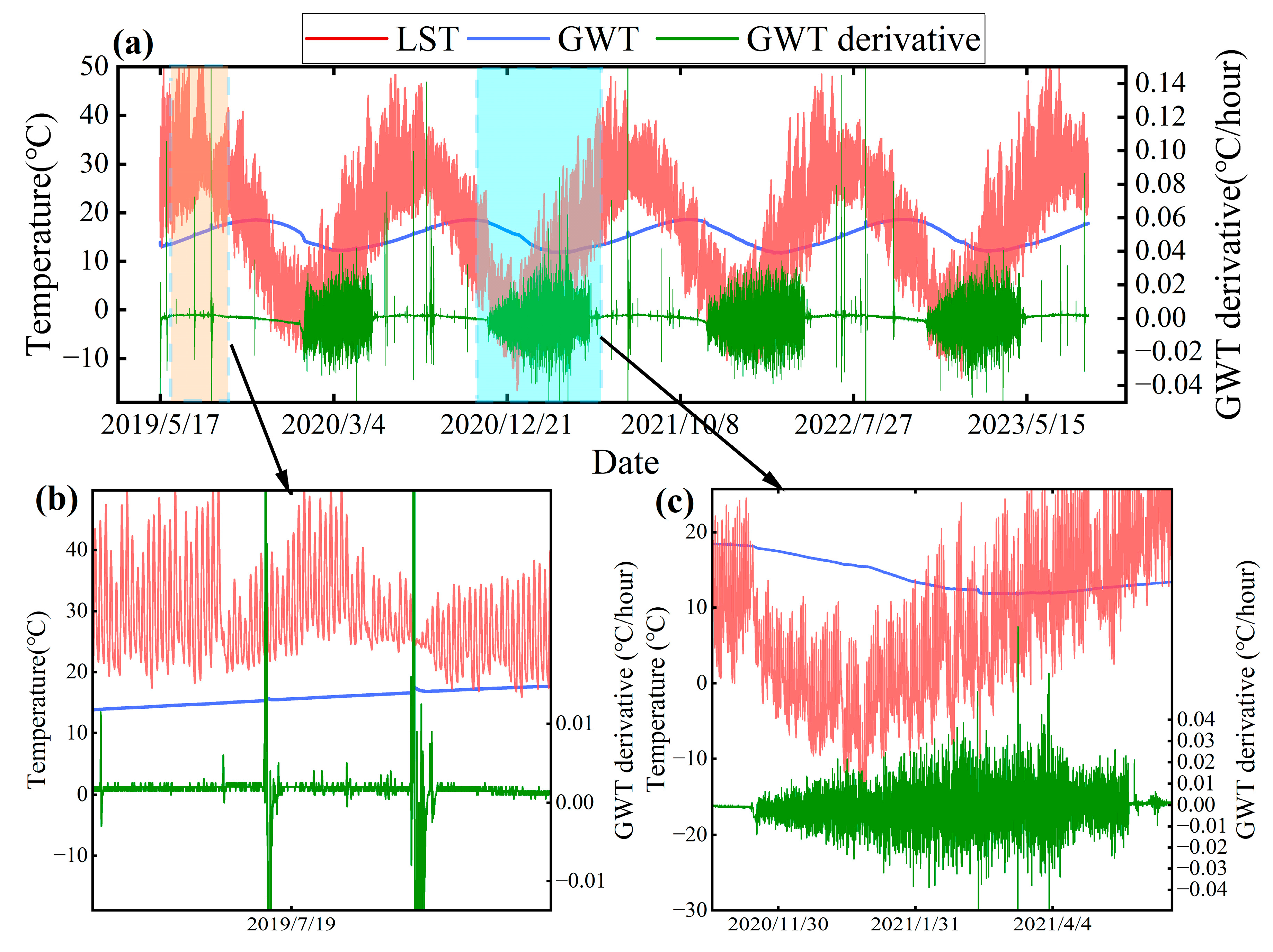
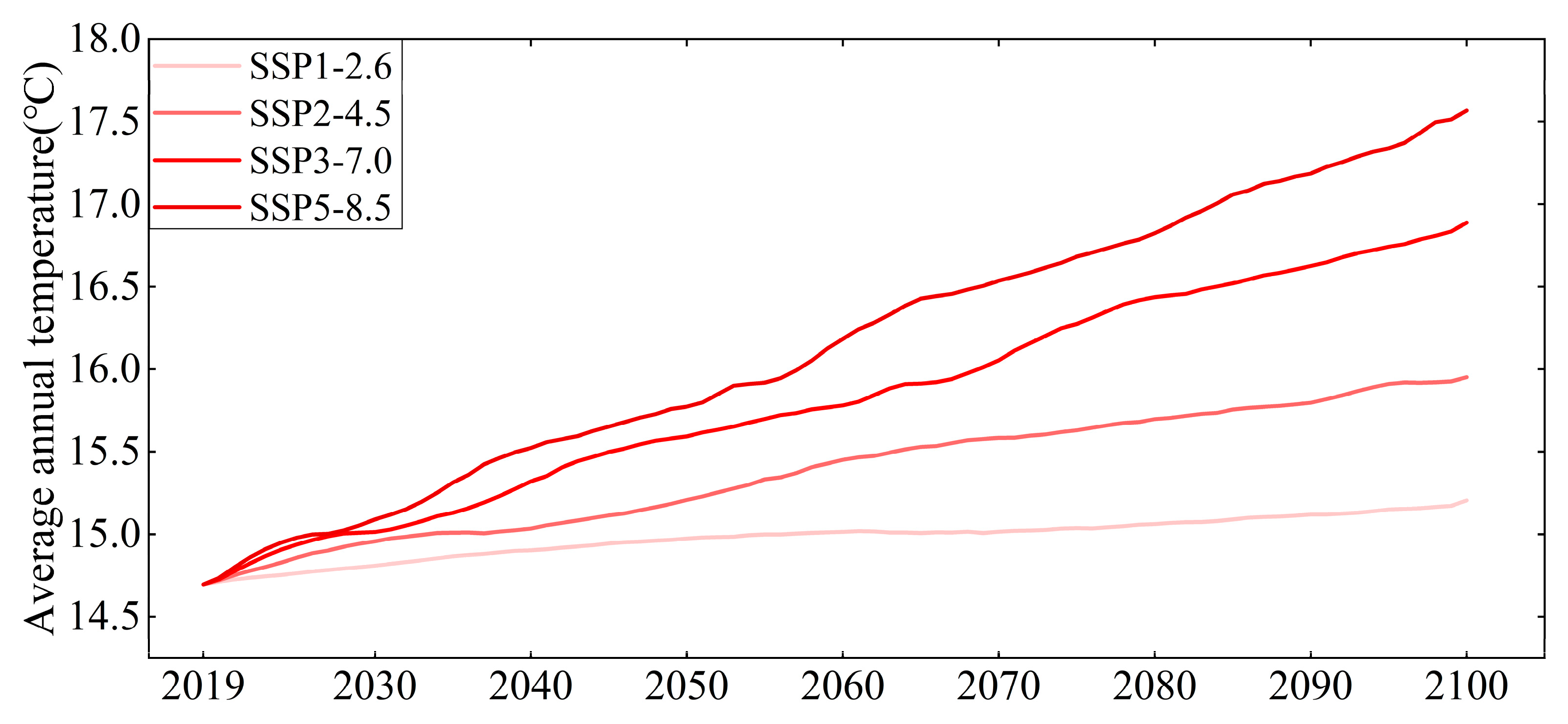
3.2. Impact of Surface Temperature on Coastal Shallow Groundwater Temperature Under Climate Change

Surface temperature acts as the primary driver of shallow groundwater thermal dynamics, with its fluctuations directly propagating into subsurface temperature regimes. Climate change-induced global warming has significantly elevated GWTs [4]. The IPCC’s Sixth Assessment Report (AR6) confirms substantial groundwater warming attributable to climatic shifts. CMIP6 projections under the Shared Socioeconomic Pathways (SSPs) reveal distinct surface warming trajectories: SSP1-2.6 (1.18 °C/century), SSP2-4.5 (3.22 °C/century), SSP3-7.0 (5.50 °C/century), and SSP5-8.5 (7.20 °C/century) [45]. To assess groundwater thermal responses, we simulated the temperature evolution in Monitoring Well 2# under these SSP scenarios, assuming a constant GWL at historical average levels and linear surface temperature increases from 2019 baseline levels at respective SSP rates. We selected Monitoring Well 2# for this simulation analysis because its observed temperature remained relatively stable, free from anthropogenic influences and natural extreme rainfall events, thereby providing clearer insights into temperature variations and their driving mechanisms.

Table 2. Parameters used for the simulation of 2#.

Parameters	Values	Unit
Porosity, p	0.5
Volumetric heat capacity of solid, $C_s$	1.59× 106	J⋅m−3⋅K−1
Volumetric heat capacity of water, $C_w$	4.18 × 106	J⋅m−3⋅K−1
Unsaturated aquifer thermal conductivity (warming),${\lambda }_{w-us}$	2.4	W·m−1·K−1
Saturated aquifer thermal conductivity (warming), ${\lambda }_{w-s}$	2.7	W·m−1·K−1
Unsaturated aquifer thermal conductivity (cooling), ${\lambda }_{c-us}$	1.05	W·m−1·K−1
Saturated aquifer thermal conductivity (cooling), ${\lambda }_{c-s}$	1.3	W·m−1·K−1
GWL variation coefficient (wetting), $k_w$	150
GWL variation coefficient (drying), $k_c$	220
Temperature gradient coefficient, $m$	0.05
Fourier number, $Fo$	0.27

presents the parameters used in the model for Monitoring Well #2, including their values and units.

Figure 8 demonstrates that GWT increases in tandem with rising surface temperatures, with the SSP1-2.6 scenario showing the smallest warming trend and SSP5-8.5 exhibiting the most pronounced temperature rise. The results confirm a positive correlation between groundwater warming rates and surface temperature escalation—the faster the surface warms, the quicker GWTs climb. By 2100, the projected GWT increases under each scenario are as follows: ~0.51 °C for SSP1-2.6, ~1.25 °C for SSP2-4.5, ~2.19 °C for SSP3-7.0, and ~2.87 °C for SSP5-8.5. These findings align with the predictions by Benz et al. [4], who estimated an average groundwater warming of 2.1 °C under a medium emission pathway.

To investigate the impact of short-term extreme temperature fluctuations on GWT, we artificially increased the surface temperatures by 3 °C during both the warmest three-month period (July–September) and the coldest three-month period (December–February) at the monitoring well site. This experimental design allowed the observation of groundwater thermal responses to transient surface temperature anomalies, specifically assessing the timing (onset) and temporal scope (duration) of the thermal effects triggered by abrupt seasonal warming/cooling perturbations in shallow aquifers.

Figure 9a,b demonstrate that when surface temperature peaks (summer) and troughs (winter) are artificially elevated, corresponding increases occur in the GWT peaks and troughs. Notably, surface temperature peaks and troughs primarily occur in July–August–September and December–January–February, respectively, while GWT peaks and troughs lag behind, emerging in October–November–December and March–April–May. This indicates a delayed response of GWT to surface thermal perturbations, with a time lag of approximately three months. This hysteresis aligns with classical subsurface heat transfer principles, traditionally described as “phase lag” in analytical solutions that model surface temperature as cosine functions. However, such idealized formulations fail to capture the transient thermal impacts caused by short-term temperature spikes. A comparative analysis reveals distinct groundwater responses to seasonal heating: identical 3 °C LST increases applied during the winter trough months (December–January–February 2021) induce increased groundwater warming (peak rise ~0.95 °C) compared to equivalent summer peak heating (July–August–September 2020, peak rise ~0.41 °C). Furthermore, thermal perturbations exhibit phase-dependent sensitivity—maximum GWT shifts occur when surface heating coincides with natural temperature extremes (peaks/troughs), with diminishing effects as interventions deviate from these critical periods. Meanwhile, short-term surface heating also propagates downstream in the thermal cycle, elevating subsequent seasonal peaks/troughs within the same annual cycle and generating cascading thermal impacts throughout the year.

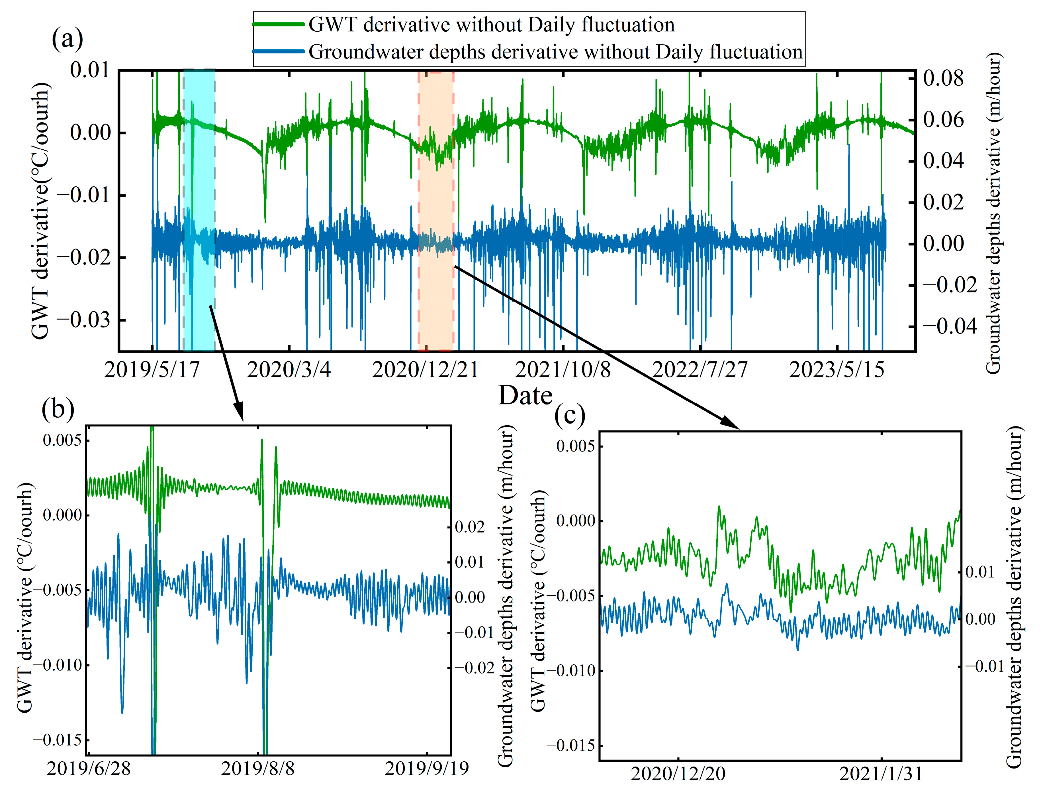
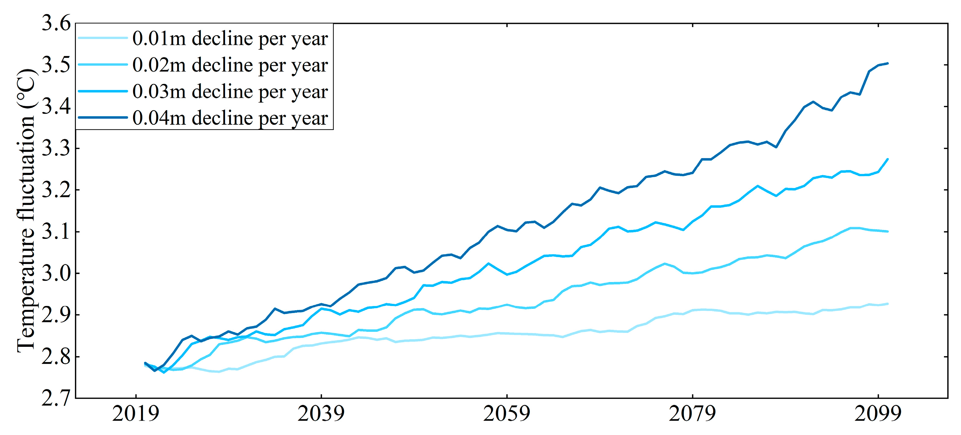
3.3. Impact of Groundwater Levels on Coastal Shallow Groundwater Temperature Under Climate Change

Under climate change, global groundwater resources are depleting. Over the past 40 years, 30% of regional aquifers worldwide have experienced an accelerated GWL decline [46]. The anthropogenic overexploitation and utilization of groundwater are recognized as primary drivers of this decline [46,47,48]. Rates of GWL reduction vary across regions and under different human-induced conditions. Bera et al. [49] demonstrated that unconfined hard rock aquifers in the extended Chota Nagpur Plateau, India, exhibited GWL decline rates ranging from −0.006 to −0.205 m/year during their monsoon seasons and −0.005 to −0.192 m/year in non-monsoon periods between 1996 and 2017. Le Brocque et al. [50] reported an average annual GWL decline of 0.06 m in southern Queensland, Australia, over 26 years (1989–2015). Under the SSP5–8.5 scenario, Panahi et al. [51] projected a 6.60 m reduction in the Mashhad aquifer (2022–2064), while Dong et al. [52] identified an annual 0.06 m decline trend in agricultural areas of the U.S. Mid-Atlantic region. Contrastingly, Silva et al. [53] observed GWL recovery in southwestern Europe due to improved management practices. In arid climate zones with intensive agriculture, groundwater depletion rates can exceed 0.5 m/year [46]. Coastal shallow groundwater dynamics remain controversial. Some studies attribute rising shallow GWLs to seawater intrusion and sea-level rise [54,55], while others suggest persistent declining trends in coastal zones [56,57,58]. Previous research on the Yellow River Delta indicates a general decline in coastal shallow GWLs [56,58]. To investigate how climate-driven groundwater depletion affects shallow aquifer thermal regimes, we simulated GWT responses under four progressive decline scenarios (0.01, 0.02, 0.03, and 0.04 m/year) throughout the year 2100, assuming a constant surface temperature. The analysis focused on temperature variations at a 7 m depth in Monitoring Well 2#.

Figure 10 presents the relationship between GWT fluctuations and their temporal variations, showing that these fluctuations intensify with decreasing GWLs, with distinct variations observed across different rates of GWL decline. This indicates that lower GWLs lead to greater thermal instability in groundwater systems. The mechanism behind this lies in the influence of GWLs on subsurface thermal diffusivity: a decline in GWLs increases thermal diffusivity, thereby amplifying temperature fluctuations. By 2100, the projected increases in GWT fluctuations under the different scenarios are projected at approximately 0.094 °C (0.01 m/year decline rate), 0.27 °C (0.02 m/year), 0.44 °C (0.03 m/year), and 0.67 °C (0.04 m/year), demonstrating a clear dependency of thermal variability on both the magnitude and velocity of water level reduction.

To investigate how short-term GWL variations affect GWT, we removed GWL fluctuations from June to October to create a modified GWL dataset. By comparing the simulation results using measured GWLs with those using the modified dataset (after removing rainy-season precipitation), we analyzed the differences between seasonal GWL changes and idealized steady-state conditions without fluctuations, as well as their impacts on temperature.

Figure 11 presents simulated temperature results under scenarios with and without rainy-season water level fluctuations in the study area (Yellow River Delta), characterized by a warm–temperate semi-humid continental monsoon climate with concurrent rainfall and high temperatures in summer, typically causing significant seasonal water level variations. By removing rainy-season GWL fluctuations and maintaining a stable water table, the simulation reveals that seasonal rainfall dynamically regulates GWT. Eliminating rainy-season fluctuations induces an overall temperature increase near peak values, attributable to reduced subsurface thermal diffusivity under elevated water levels, which diminishes heat transfer from surface temperatures to deeper zones. During this period, GWTs become warmer and reduced thermal diffusivity leads to lower peaks. These findings indicate that rainy-season precipitation-induced water level elevation may enhance subsurface thermal stability by moderating heat exchange dynamics.

4. Discussion

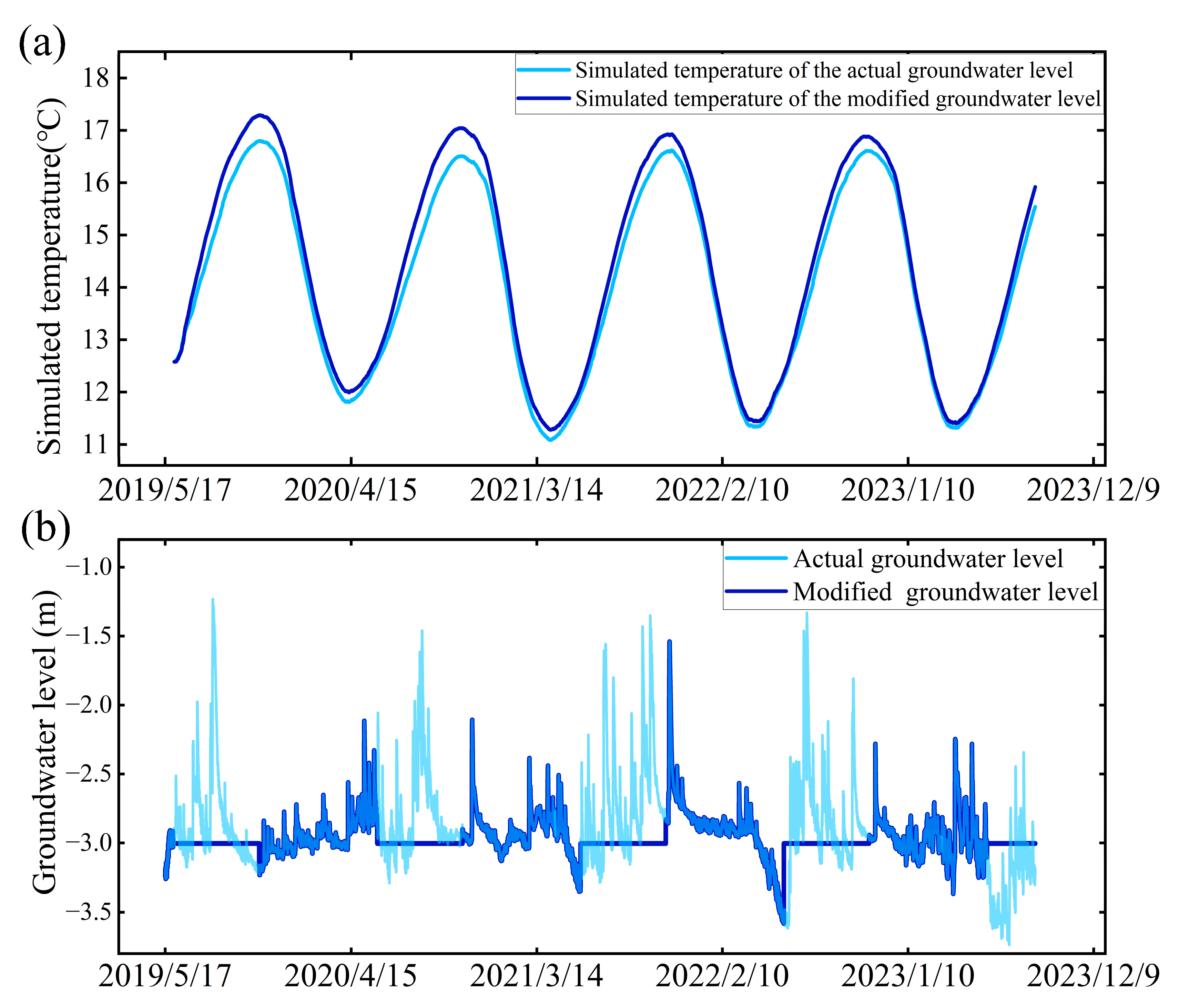
4.1. Differences in Shallow Groundwater Temperature Responses to Short-Term Natural Extreme Rainfall and Anthropogenic Agricultural Activities

Short-duration, high-intensity rainfall can cause significant temperature changes in shallow groundwater, with heavy rainfall introducing strong thermal signals that alter GWTs [59]. Figure 12a displays the temperature, GWL, and rainfall data from Monitoring Well 6#, which experienced an extreme precipitation event on 12 July 2022. The observed GWL rose rapidly by approximately 1.67 m, accompanied by a short-term temperature increase of about 4.4 °C. However, such rainfall-induced thermal changes typically re-equilibrate within days. Luo et al. [60] also reported elevated temperatures in shallow groundwater during extreme summer storms, likely due to large influxes of warmer recharge water into the aquifer system. Temporal variations in concentrated recharge rates during rainfall events remain difficult to quantify and depend heavily on precipitation intensity and duration. The impact on GWT varies with these factors—for example, a more intense but shorter rainfall event on 2 October 2022 caused no detectable thermal response, demonstrating differential effects based on rainfall characteristics.

Beyond natural rainfall impacts, human activities also influence GWT. Studies indicate that subsurface infrastructure modifications and urban heat island effects can alter groundwater thermal regimes [61,62]. Additionally, we observe agricultural land use impacts: Figure 13 displays data from Monitoring Well 7#, where temperature fluctuations, characterized by sudden spikes, occur annually in February and March. These temperature anomalies may be linked to localized agricultural management practices. This monitoring well is situated adjacent to farmland implementing a unique reed–crop rotation system: annual early-spring (February–March) controlled burning removes invasive reeds (dominant vegetation in the Yellow River Delta wetland ecosystem), followed by Yellow River diversion irrigation and crop cultivation. This anthropogenic factor of burning and diversion of surface water for irrigation may be the cause of the abnormal GWT. Monitoring data confirm that abrupt increases in the GWL without corresponding rainfall are accompanied by increases in temperature. Benz et al. [63] similarly found elevated GWTs in cultivated areas, hypothesizing links to irrigation with thermally altered surface water.

A comparative analysis of Figure 12 and Figure 13 reveals distinct recovery timescales for thermal anomalies under natural versus human-induced conditions. Temperature perturbations caused by artificial irrigation exhibit significantly prolonged recovery periods (months) compared to natural precipitation-driven fluctuations (days). While intense rainfall events can induce abrupt temperature spikes (e.g., +4.4 °C), these rapidly re-equilibrate through natural hydrological processes within a few days. In contrast, irrigation-associated thermal anomalies demonstrate extended persistence. Our modeling framework, which excludes advective heat transport and assumes purely conductive processes, effectively delineates the spatiotemporal boundaries of thermal impacts, enabling a quantitative separation of natural extreme precipitation and anthropogenic irrigation effects on groundwater thermal regimes.

4.2. Potential Impacts of Future Groundwater Temperature Changes Under Climate Change

Under the influence of human activities, the impacts of future global climate change may be more severe than previously estimated, with the pace of climate change accelerating (IPCC AR6). By 2050, approximately 35% of the Earth’s habitable areas may become uninhabitable due to rising temperatures [64]. The two most significant climate change impacts in the future will be (1) global temperature increases and (2) an increased frequency of extreme weather events. Both factors are likely to alter GWT dynamics. A scientific consensus formed that global warming will lead to rising GWTs worldwide and accelerate groundwater resource depletion [4,65,66]. Prolonged surface temperature increases coupled with declining GWLs may cause both GWT elevation (Result 3.4) and intensified thermal fluctuations (Result 3.5). Elevated temperatures and expanded thermal ranges could jeopardize stenothermic organisms specialized to narrow thermal niches [67], potentially devastating aquifer-dependent ecosystems [68,69,70]. Additionally, groundwater quality may degrade as warmer conditions accelerate microbial metabolism, shifting aquifers from oxic to anoxic states and altering geochemical processes [5,10,15]. Modified chemical characteristics in coastal aquifers may subsequently influence marine chemistry through submarine groundwater discharge. For instance, temperature-mediated phosphate release into coastal waters could fuel algal blooms by providing excessive nutrients [71], with seasonal water temperature variations being a key driver of bloom risks [72]. Furthermore, extreme surface temperature anomalies (both high and low) may amplify GWT peaks and troughs (Result 3.4). During warm summers, cold groundwater discharge typically provides critical thermal refugia for endangered salmonids and other aquatic species, but rising GWTs threaten these habitats [73]. The brook trout (Salvelinus fontinalis), an ecologically, economically, and culturally valuable cold-water species particularly sensitive to stream warming, faces habitat loss from either groundwater warming or reduced discharge. In temperate–cold climate transition zones, abrupt winter warming may diminish groundwater recharge rates [74]. Although short-term rainfall events may temporarily stabilize GWTs (Result 3.5), future precipitation patterns are projected to become more extreme, with intense rainfall concentrating in wet seasons and severe droughts occurring in dry seasons [75]. This rainfall redistribution will amplify seasonal GWL fluctuations [74], potentially widening the water level difference between the wet and dry seasons. Such intensified seasonal GWL variations may destabilize GWTs during drought periods, particularly in arid seasons.

5. Conclusions

Based on multi-year hourly observation data, we constructed a high-precision numerical model with hourly resolution to analyze dynamic changes in GWT at short time scales. This study found significant differences in the dominant influencing factors during GWT warming and cooling periods. This model innovatively achieves a dynamic inversion of thermal diffusivity through real-time coupled calculations of GWL and temperature gradients, eliminating the need for the direct measurement of soil–rock thermal properties, but instead requiring high-temporal-resolution temperature monitoring data (obtainable through low-cost sensors). The model design focuses on quantifying seasonal temperature variations, revealing the mechanisms by which GWL fluctuations and surface temperature affect GWT through multi-temporal scale analysis. Using scenario simulation methods, this study successfully predicted the differential thermal response characteristics of coastal shallow groundwater systems to short-term extreme events (rainstorm infiltration and abnormal high temperatures) and long-term stressors (rising average surface temperatures and global GWL decline) under climate change. It identified that GWL decline will trigger enhanced temperature fluctuations. This modeling framework provides new tool support for research on groundwater thermal processes under climate change.

References

1. Amanambu, A.C.; Obarein, O.A.; Mossa, J.; Li, L.H.; Ayeni, S.S.; Balogun, O.; Oyebamiji, A.; Ochege, F.U. Groundwater system and climate change: Present status and future considerations. J. Hydrol. 2020, 589, 125163. [Google Scholar] [CrossRef]
2. Kuang, X.X.; Liu, J.G.; Scanlon, B.R.; Jiao, J.J.; Jasechko, S.; Lancia, M.; Biskaborn, B.K.; Wada, Y.; Li, H.L.; Zeng, Z.Z.; et al. The changing nature of groundwater in the global water cycle. Science 2024, 383, eadf0630. [Google Scholar] [CrossRef] [PubMed]
3. Kurylyk, B.L.; MacQuarrie, K.T.B.; Caissie, D.; McKenzie, J.M. Shallow groundwater thermal sensitivity to climate change and land cover disturbances: Derivation of analytical expressions and implications for stream temperature modeling. Hydrol. Earth Syst. Sci. 2015, 19, 2469–2489. [Google Scholar] [CrossRef]
4. Benz, S.A.; Irvine, D.J.; Rau, G.C.; Bayer, P.; Menberg, K.; Blum, P.; Jamieson, R.C.; Griebler, C.; Kurylyk, B.L. Global groundwater warming due to climate change. Nat. Geosci. 2024, 17, 545–551. [Google Scholar] [CrossRef]
5. Riedel, T. Temperature-associated changes in groundwater quality. J. Hydrol. 2019, 572, 206–212. [Google Scholar] [CrossRef]
6. Saito, T.; Hamamoto, S.; Ueki, T.; Ohkubo, S.; Moldrup, P.; Kawamoto, K.; Komatsu, T. Temperature change affected groundwater quality in a confined marine aquifer during long-term heating and cooling. Water Res. 2016, 94, 120–127. [Google Scholar] [CrossRef]
7. Price, P.B.; Sowers, T. Temperature dependence of metabolic rates for microbial growth, maintenance, and survival. Proc. Natl. Acad. Sci. USA 2004, 101, 4631–4636. [Google Scholar] [CrossRef]
8. Jorgensen, C.J.; Jacobsen, O.S.; Elberling, B.; Aamand, J. Microbial Oxidation of Pyrite Coupled to Nitrate Reduction in Anoxic Groundwater Sediment. Environ. Sci. Technol. 2009, 43, 4851–4857. [Google Scholar] [CrossRef]
9. Addy, K.; Gold, A.J.; Christianson, L.E.; David, M.B.; Schipper, L.A.; Ratigan, N.A. Denitrifying Bioreactors for Nitrate Removal: A Meta-Analysis. J. Environ. Qual. 2016, 45, 873–881. [Google Scholar] [CrossRef]
10. Cogswell, C.; Heiss, J.W. Climate and Seasonal Temperature Controls on Biogeochemical Transformations in Unconfined Coastal Aquifers. J. Geophys. Res.-Biogeosciences 2021, 126, e2021JG006605. [Google Scholar] [CrossRef]
11. Menberg, K.; Blum, P.; Kurylyk, B.L.; Bayer, P. Observed groundwater temperature response to recent climate change. Hydrol. Earth Syst. Sci. 2014, 18, 4453–4466. [Google Scholar] [CrossRef]
12. Saito, H.; Simunek, J.; Mohanty, B.P. Numerical analysis of coupled water, vapor, and heat transport in the vadose zone. Vadose Zone J. 2006, 5, 784–800. [Google Scholar] [CrossRef]
13. Mandavi, S.M.; Neyshabouri, M.R.; Fujimaki, H. Water vapour transport in a soil column in the presence of an osmotic gradient. Geoderma 2018, 315, 199–207. [Google Scholar] [CrossRef]
14. Green, T.R.; Taniguchi, M.; Kooi, H.; Gurdak, J.J.; Allen, D.M.; Hiscock, K.M.; Treidel, H.; Aureli, A. Beneath the surface of global change: Impacts of climate change on groundwater. J. Hydrol. 2011, 405, 532–560. [Google Scholar] [CrossRef]
15. Neidhardt, H.; Shao, W. Impact of climate change-induced warming on groundwater temperatures and quality. Appl. Water Sci. 2023, 13, 235. [Google Scholar] [CrossRef]
16. Bense, V.F.; Kurylyk, B.L.; Bruin, J.G.H.; Visser, P. Repeated Subsurface Thermal Profiling to Reveal Temporal Variability in Deep Groundwater Flow Conditions. Water Resour. Res. 2020, 56, e2019WR026913. [Google Scholar] [CrossRef]
17. Arias-Penas, D.; Castro-García, M.P.; Rey-Ronco, M.A.; Alonso-Sánchez, T. Determining the thermal diffusivity of the ground based on subsoil temperatures. Preliminary results of an experimental geothermal borehole study Q-THERMIE-UNIOVI. Geothermics 2015, 54, 35–42. [Google Scholar] [CrossRef]
18. Liu, Q.Y.; Chen, S.Y.; Zhou, B. Estimating temporal patterns of vertical groundwater flux using multidepth temperature time series: A numerical method. J. Hydrol. 2024, 639, 131623. [Google Scholar] [CrossRef]
19. García-Pereira, F.; González-Rouco, J.F.; Schmid, T.; Melo-Aguilar, C.; Vegas-Cañas, C.; Steinert, N.J.; Roldan-Gómez, P.J.; Cuesta-Valero, F.J.; García-García, A.; Beltrami, H.; et al. Thermodynamic and hydrological drivers of the soil and bedrock thermal regimes in central Spain. Soil 2024, 10, 1–21. [Google Scholar] [CrossRef]
20. Rau, G.C.; Halloran, L.J.S.; Cuthbert, M.O.; Andersen, M.S.; Acworth, R.I.; Tellam, J.H. Characterising the dynamics of surface water-groundwater interactions in intermittent and ephemeral streams using streambed thermal signatures. Adv. Water Resour. 2017, 107, 354–369. [Google Scholar] [CrossRef]
21. Malik, M.S.; Shukla, J.P.; Mishra, S. Effect of Groundwater Level on Soil Moisture, Soil Temperature and Surface Temperature. J. Indian. Soc. Remote 2021, 49, 2143–2161. [Google Scholar] [CrossRef]
22. Campbell, G.S.; Jungbauer, J.D.; Bidlake, W.R.; Hungerford, R.D. Predicting the Effect of Temperature on Soil Thermal-Conductivity. Soil. Sci. 1994, 158, 307–313. [Google Scholar] [CrossRef]
23. Boukelia, A.; Eslami, H.; Rosin-Paumier, S.; Masrouri, F. Effect of temperature and initial state on variation of thermal parameters of fine compacted soils. Eur. J. Environ. Civ. Eng. 2019, 23, 1125–1138. [Google Scholar] [CrossRef]
24. Van Wijk, W.R.; De Vries, D.A. Periodic Temperature Variations in a Homogeneous Soil; North-Holland: Amsterdam, The Netherland, 1963; pp. 103–143. [Google Scholar]
25. Carslaw, H.; Jaeger, J. Conduction of Heat in Solids, 2nd ed.; Oxford University Press: New York, NY, USA, 1959; p. 510. [Google Scholar]
26. Hatch, C.E.; Fisher, A.T.; Revenaugh, J.S.; Constantz, J.; Ruehl, C. Quantifying surface water-groundwater interactions using time series analysis of streambed thermal records: Method development. Water Resour. Res. 2006, 42, e2005w10410. [Google Scholar] [CrossRef]
27. Keery, J.; Binley, A.; Crook, N.; Smith, J.W.N. Temporal and spatial variability of groundwater-surface water fluxes: Development and application of an analytical method using temperature time series. J. Hydrol. 2007, 336, 1–16. [Google Scholar] [CrossRef]
28. McCallum, A.M.; Andersen, M.S.; Rau, G.C.; Acworth, R.I. A 1-D analytical method for estimating surface water-groundwater interactions and effective thermal diffusivity using temperature time series. Water Resour. Res. 2012, 48, e2012w11532. [Google Scholar] [CrossRef]
29. Luce, C.H.; Tonina, D.; Gariglio, F.; Applebee, R. Solutions for the diurnally forced advection-diffusion equation to estimate bulk fluid velocity and diffusivity in streambeds from temperature time series. Water Resour. Res. 2013, 49, 488–506. [Google Scholar] [CrossRef]
30. Vandersteen, G.; Schneidewind, U.; Anibas, C.; Schmidt, C.; Seuntjens, P.; Batelaan, O. Determining groundwater-surface water exchange from temperature-time series: Combining a local polynomial method with a maximum likelihood estimator. Water Resour. Res. 2015, 51, 922–939. [Google Scholar] [CrossRef]
31. Kampen, R.; Schneidewind, U.; Anibas, C.; Bertagnoli, A.; Tonina, D.; Vandersteen, G.; Luce, C.; Krause, S.; Berkel, M. LPMLE-A Frequency Domain Method to Estimate Vertical Streambed Fluxes and Sediment Thermal Properties in Semi-Infinite and Bounded Domains. Water Resour. Res. 2022, 58, e2021WR030886. [Google Scholar] [CrossRef]
32. Shi, W.G.; Wang, Q.R.; Klepikova, M.; Irvine, D.J.; Rashed, A.; Liao, Z.L. BDFLUX: A new bounded domain model for quantifying vertical fluxes in streambeds using heat as a tracer. J. Hydrol. 2024, 633, 130981. [Google Scholar] [CrossRef]
33. Dong, Y.; McCartney, J.S.; Lu, N. Critical Review of Thermal Conductivity Models for Unsaturated Soils. Geotech. Geol. Eng. 2015, 33, 207–221. [Google Scholar] [CrossRef]
34. Ghanbarian, B.; Daigle, H. Thermal conductivity in porous media: Percolation-based effective-medium approximation. Water Resour. Res. 2016, 52, 295–314. [Google Scholar] [CrossRef]
35. Zhang, N.; Wang, Z.Y. Review of soil thermal conductivity and predictive models. Int. J. Therm. Sci. 2017, 117, 172–183. [Google Scholar] [CrossRef]
36. Lu, S.; Ren, T.S.; Gong, Y.S.; Horton, R. An improved model for predicting soil thermal conductivity from water content at room temperature. Soil. Sci. Soc. Am. J. 2007, 71, 8–14. [Google Scholar] [CrossRef]
37. He, H.L.; Zhao, Y.; Dyck, M.F.; Si, B.C.; Jin, H.J.; Lv, J.L.; Wang, J.X. A modified normalized model for predicting effective soil thermal conductivity. Acta Geotech. 2017, 12, 1281–1300. [Google Scholar] [CrossRef]
38. Tarnawski, V.R.; Gori, F.; Wagner, B.; Buchan, G.D. Modelling approaches to predicting thermal conductivity of soils at high temperatures. Int. J. Energ. Res. 2000, 24, 403–423. [Google Scholar] [CrossRef]
39. Rau, G.C.; Andersen, M.S.; Acworth, R.I. Experimental investigation of the thermal dispersivity term and its significance in the heat transport equation for flow in sediments. Water Resour. Res. 2012, 48, e2011wr011038. [Google Scholar] [CrossRef]
40. Abu-Hamdeh, N.H.; Reeder, R.C. Soil thermal conductivity: Effects of density, moisture, salt concentration, and organic matter. Soil. Sci. Soc. Am. J. 2000, 64, 1285–1290. [Google Scholar] [CrossRef]
41. Bittelli, M.; Ventura, F.; Campbell, G.S.; Snyder, R.L.; Gallegati, F.; Pisa, P.R. Coupling of heat, water vapor, and liquid water fluxes to compute evaporation in bare soils. J. Hydrol. 2008, 362, 191–205. [Google Scholar] [CrossRef]
42. Du, C.Y.; Yu, J.J.; Wang, P.; Zhang, Y.C. Analysing the mechanisms of soil water and vapour transport in the desert vadose zone of the extremely arid region of northern China. J. Hydrol. 2018, 558, 592–606. [Google Scholar] [CrossRef]
43. Rondanelli, R.; Molina, A.; Falvey, M. The Atacama Surface Solar Maximum. Bull. Am. Meteorol. Soc. 2015, 96, 405–418. [Google Scholar] [CrossRef]
44. Jing, W.Q.; Wang, J.F. A Dynamics of Surface Temperature Forced by Solar Radiation. Geophys. Res. Lett. 2023, 50, e2022GL101222. [Google Scholar] [CrossRef]
45. Fan, X.W.; Duan, Q.Y.; Shen, C.W.; Wu, Y.; Xing, C. Global surface air temperatures in CMIP6: Historical performance and future changes. Environ. Res. Lett. 2020, 15, 104056. [Google Scholar] [CrossRef]
46. Jasechko, S.; Seybold, H.; Perrone, D.; Fan, Y.; Shamsudduha, M.; Taylor, R.G.; Fallatah, O.; Kirchner, J.W. Rapid groundwater decline and some cases of recovery in aquifers globally. Nature 2024, 625, 715–721. [Google Scholar] [CrossRef]
47. Sharma, C.; Basagaoglu, H.; Yoosefdoost, I.; Wootten, A.; Chakraborty-Reddy, D.; Bertetti, F.P.; Mirchi, A.; Chakraborty, D. Efficacy of mitigation strategies for aquifer sustainability under climate change. Nat. Sustain. 2025, 8, 44–53. [Google Scholar] [CrossRef]
48. Gordu, F.; Nachabe, M.H. Inferences of Groundwater Response to Projected Hydroclimatic Changes in North Florida. J. Hydrol. Eng. 2023, 28, 04023001. [Google Scholar] [CrossRef]
49. Bera, B.; Shit, P.K.; Sengupta, N.; Saha, S.; Bhattacharjee, S. Steady declining trend of groundwater table and severe water crisis in unconfined hard rock aquifers in extended part of Chota Nagpur Plateau, India. Appl. Water Sci. 2022, 12, 31. [Google Scholar] [CrossRef]
50. Le Brocque, A.F.; Kath, J.; Reardon-Smith, K. Chronic groundwater decline: A multi-decadal analysis of groundwater trends under extreme climate cycles. J. Hydrol. 2018, 561, 976–986. [Google Scholar] [CrossRef]
51. Panahi, G.; Eskafi, M.H.; Faridhosseini, A.; Khodashenas, S.R.; Rohani, A. Prediction of groundwater level fluctuations under climate change based on machine learning algorithms in the Mashhad Aquifer, Iran. J. Water Clim. Change 2023, 14, 1039–1059. [Google Scholar] [CrossRef]
52. Dong, Y.; Jiang, C.S.; Suri, M.R.; Pee, D.; Meng, L.K.; Goldstein, R.E.R. Groundwater level changes with a focus on agricultural areas in the Mid-Atlantic region of the United States, 2002–2016. Environ. Res. 2019, 171, 193–203. [Google Scholar] [CrossRef]
53. Silva, R.C.G.; Reinecke, R.; Copty, N.K.; Barry, D.A.; Heggy, E.; Labat, D.; Roggero, P.P.; Borchardt, D.; Rode, M.; Gómez-Hernández, J.J.; et al. Multi-decadal groundwater observations reveal surprisingly stable levels in southwestern Europe. Commun. Earth Environ. 2024, 5, 387. [Google Scholar] [CrossRef]
54. Song, S.H.; Zemansky, G. Groundwater level fluctuation in the Waimea Plains, New Zealand: Changes in a coastal aquifer within the last 30 years. Environ. Earth Sci. 2013, 70, 2167–2178. [Google Scholar] [CrossRef]
55. O’Driscoll, M.; Humphrey, C.J.r.; Iverson, G.; Bowden, J.; Harrison, J. Rising groundwater levels in Dare County, North Carolina: Implications for onsite wastewater management for coastal communities. J. Water Clim. Change 2024, 15, 3666–3688. [Google Scholar] [CrossRef]
56. Fan, X.M.; Min, T.; Dai, X.J. The Spatio-Temporal Dynamic Patterns of Shallow Groundwater Level and Salinity: The Yellow River Delta, China. Water 2023, 15, 1426. [Google Scholar] [CrossRef]
57. Panda, D.K.; Mishra, A.; Kumar, A. Quantification of trends in groundwater levels of Gujarat in western India. Hydrol. Sci. J. 2012, 57, 1325–1336. [Google Scholar] [CrossRef]
58. Zhang, Y.; Wang, J.C.; Jing, J.H.; Sun, J.C. Response of groundwater to climate change under extreme climate conditions in North China Plain. J. Earth Sci. 2014, 25, 612–618. [Google Scholar] [CrossRef]
59. Chen, K.W.; Guo, Z.L.; Yin, M.S.; Liang, X.Y.; Chang, Z.B.; Yang, S.; Wei, X.O.; Zhai, X.C.; Zheng, C.M. Using Rainfall-Induced Groundwater Temperature Response to Estimate Lateral Flow Velocity. Water Resour. Res. 2024, 60, e2023WR036715. [Google Scholar] [CrossRef]
60. Luo, M.M.; Wan, L.; Liao, C.L.; Jakada, H.; Zhou, H. Geographic and transport controls of temperature response in karst springs. J. Hydrol. 2023, 623, 129850. [Google Scholar] [CrossRef]
61. Benz, S.A.; Bayer, P.; Goettsche, F.M.; Olesen, F.S.; Blum, P. Linking Surface Urban Heat Islands with Groundwater Temperatures. Environ. Sci. Technol. 2016, 50, 70–78. [Google Scholar] [CrossRef]
62. Attard, G.; Rossier, Y.; Winiarski, T.; Eisenlohr, L. Deterministic modeling of the impact of underground structures on urban groundwater temperature. Sci. Total Environ. 2016, 572, 986–994. [Google Scholar] [CrossRef]
63. Benz, S.A.; Bayer, P.; Blum, P. Identifying anthropogenic anomalies in air, surface and groundwater temperatures in Germany. Sci. Total Environ. 2017, 584, 145–153. [Google Scholar] [CrossRef] [PubMed]
64. Xu, C.; Kohler, T.A.; Lenton, T.M.; Svenning, J.C.; Scheffer, M. Future of the human climate niche. Proc. Natl. Acad. Sci. USA 2020, 117, 11350–11355. [Google Scholar] [CrossRef] [PubMed]
65. Bhattarai, N.; Lobell, D.B.; Balwinder-Singh; Fishman, R.; Kustas, W.P.; Pokhrel, Y.; Jain, M. Warming temperatures exacerbate groundwater depletion rates in India. Sci. Adv. 2023, 9, eadi1401. [Google Scholar] [CrossRef]
66. Rosa, L.; Sangiorgio, M. Global water gaps under future warming levels. Nat. Commun. 2025, 16, 1192. [Google Scholar] [CrossRef]
67. Di Cicco, M.; Di Lorenzo, T.; Fiasca, B.; Galmarini, E.; Vaccarelli, I.; Cerasoli, F.; Di Camillo, A.T.; Galassi, D.M.P. Some like it hot: Thermal preference of the groundwater amphipod Niphargus longicaudatus (Costa, 1851) and climate change implications. J. Therm. Biol. 2023, 116, 103654. [Google Scholar] [CrossRef]
68. Benjamin, J.R.; Heltzel, J.M.; Dunham, J.B.; Heck, M.; Banish, N. Thermal Regimes, Nonnative Trout, and Their Influences on Native Bull Trout in the Upper Klamath River Basin, Oregon. Trans. Am. Fish. Soc. 2016, 145, 1318–1330. [Google Scholar] [CrossRef]
69. Griebler, C.; Brielmann, H.; Haberer, C.M.; Kaschuba, S.; Kellermann, C.; Stumpp, C.; Hegler, F.; Kuntz, D.; Walker-Hertkorn, S.; Lueders, T. Potential impacts of geothermal energy use and storage of heat on groundwater quality, biodiversity, and ecosystem processes. Environ. Earth Sci. 2016, 75, 1391. [Google Scholar] [CrossRef]
70. Castaño-Sánchez, A.; Hose, G.C.; Reboleira, A.S.P.S. Salinity and temperature increase impact groundwater crustaceans. Sci. Rep. 2020, 10, 12328. [Google Scholar] [CrossRef]
71. Cheng, K.H.; Jiao, J.J.; Lee, J.H.W.; Luo, X. Synergistic controls of water column stability and groundwater phosphate on coastal algal blooms. Water Res. 2024, 255, 121467. [Google Scholar] [CrossRef]
72. Tong, Y.; Lei, K.; Wang, L.; Li, Y.; Lan, W.; Cheng, Y.; Deng, Z.A.; Zhai, J.; Huang, Z. Spatial-temporal characteristics and the importance of environmental factors in relation to algal blooms in coastal seas. Sci. Total Environ. 2024, 957, 177686. [Google Scholar] [CrossRef]
73. Kurylyk, B.L.; MacQuarrie, K.T.B.; Voss, C.I. Climate change impacts on the temperature and magnitude of groundwater discharge from shallow, unconfined aquifers. Water Resour. Res. 2014, 50, 3253–3274. [Google Scholar] [CrossRef]
74. Nygren, M.; Giese, M.; Kløve, B.; Haaf, E.; Rossi, P.M.; Barthel, R. Changes in seasonality of groundwater level fluctuations in a temperate-cold climate transition zone. J. Hydrol. X 2020, 8, 100062. [Google Scholar] [CrossRef]
75. Sun, Q.H.; Zhang, X.B.; Zwiers, F.; Westra, S.; Alexander, L. A Global, Continental, and Regional Analysis of Changes in Extreme Precipitation. J. Clim. 2021, 34, 243–258. [Google Scholar] [CrossRef]
Figure 1. (a) Different patterns of GWT change. This Figure shows the LST and GWT, as well as the rate of change of the GWT at Monitoring Well 2#. The time period covered in this Figure is from 17 May 2019 to 26 August 2023. (b) GWT’s smooth changes in the warming phase. (c) GWT’s dramatic changes in cooling phase.
Water 17 01107 g001
Figure 2. (a) GWT and groundwater depth change rates. The derivatives of temperature and groundwater depth were processed to remove the irregular fluctuations within a day. The green line represents the variation in the temperature change rate over time, while the blue line indicates the value of the groundwater depth’s change rate. These data are also from Monitoring Well 2#. (b) Patterns of change during the warming phase. (c) Patterns of change during the cooling phase.
Water 17 01107 g002
Figure 3. Location map of the study area and monitoring wells.
Water 17 01107 g003
Figure 4. Comparison of simulation results with measured data by numerical simulation methods. (al) represent the validation results for Monitoring Wells 1# to 12#, respectively.
Water 17 01107 g004
Figure 5. Comparison of simulation results with measured data by classical analytical models. (al) represent the validation results for Monitoring Wells 1# to 12#, respectively.
Water 17 01107 g005
Figure 6. Validation of simulated and measured results at different depths in Monitoring Wells 13# and 14#.
Water 17 01107 g006
Figure 7. Vertical-direction simulation results of the simulation of the vertical annual mean temperature gradient. (a) Simulation results for Well 13# from 3 m to 6 m with intervals every 0.5 m. (b) Geothermal gradient simulation of 13# mean temperature. (c) Simulation results for Well 14# from 3 m to 6 m with intervals every 0.5 m. (d) Geothermal gradient simulation of 14# mean temperature.
Water 17 01107 g007
Figure 8. Impact of rising surface temperature on mean GWT under different SSP scenario simulations.
Water 17 01107 g008
Figure 9. (a) Changes in simulated GWTs under short-term surface temperature scenarios. (b) Original LST versus LST with a 3 °C increase in July, August, and September of 2020 and December, January, and February of 2021.
Water 17 01107 g009
Figure 10. Impact of declining GWL on GWT fluctuations under multi-scenario simulations.
Water 17 01107 g010
Figure 11. Simulation results of groundwater level impact on temperature: (a) light blue curve represents simulated temperatures under observed groundwater level conditions, while dark blue curve indicates modified simulated temperature; (b) light blue indicates measured groundwater level, and dark blue corresponds to modified groundwater level after removing fluctuations from June to October.
Water 17 01107 g011
Figure 12. GWT response to intensity natural rainfall.
Water 17 01107 g012
Figure 13. GWT response to anthropogenic irrigation.
Water 17 01107 g013