Characterization and Quantification of Fracture Roughness for Groundwater Modeling in Fractures Generated with Weierstrass–Mandelbrot Approach

Abstract

Accurate characterization of fracture roughness is critical for modeling groundwater flow and solute transport in fractured rock aquifers, where subsurface heterogeneity significantly impacts contaminant migration and water resource management. This study investigates fracture roughness characterization by integrating the Weierstrass–Mandelbrot approach with 3D-printed experimental validation and numerical simulation verification. Specifically, all the related parameters including fractal dimensions (D), frequency density (λ), segmentation accuracy (s), and summation number (n), which control the generation of fracture roughness, along with investigation scales (rs), were initially considered, and their corresponding impacts on the fracture roughness characteristics were examined. The results revealed that D is the primary factor controlling fracture roughness characteristics, while λ shows secondary importance when exceeding 1.3. The roughness remains stable when s ≤ 3 mm, n > 200, and rs ≥ 240 × 240 mm². Two multivariate regression models were established to describe the relationship between fracture roughness and influencing factors. The proposed methodology significantly enhances the precision of groundwater flow and solute transport simulations in fractured media through advanced high-fidelity fracture characterization, offering substantial improvements in groundwater resource management and contaminant remediation strategies.

1. Introduction

Compared to a fracture model of the smooth and parallel plates that maintain a consistent aperture size, the natural fractures exhibit considerable variation in fracture apertures. The surface morphology of fractures is influenced by external environmental factors, while groundwater flow, heat transfer, and solute or contaminant transport are closely related to the surface roughness and aperture size [1]. These processes are particularly crucial for groundwater resource management, as fracture characteristics significantly influence groundwater flow patterns, contaminant transport pathways, and ultimately impact water resource allocation decisions. In recent decades, research on fracture roughness has predominantly focused on groundwater flow and solute transport [2,3], unsaturated phenomena [4], and the scale sensitivity of roughness parameters alongside heat transfer [5]. Recent advances in computational capabilities have enabled detailed 3D numerical simulations for groundwater modeling, improving prediction accuracy for groundwater flow and solute transport in fractured media. These simulations serve multiple purposes essential for groundwater resource management, as demonstrated by Alberti et al., who evaluated freshwater lens distribution on small islands, and Song et al., who optimized remediation strategies for contaminated aquifers [6,7].

Machine learning has significantly enhanced the predictive capability of groundwater flow and solute transport in fractured media. However, prediction accuracy remains constrained by measurement precision and the characterization of fracture roughness at critical scales. Roughness significantly affects groundwater seepage, which in turn impacts the management of groundwater resource and contaminant transport, as well as multiphase flow regimes in oil and gas extraction. Despite these advances in computational methodologies, research on three-dimensional (3D) fracture surfaces remains limited and challenging.

Various methods exist to quantify fracture surfaces roughness, including image measurement techniques [8,9], bump height characterization, and parametric characterization of intrinsic geometric properties [10]. Additionally, the Joint Roughness Coefficient (JRC) [11] and fractal geometry methods [12,13] are also utilized. Numerous studies have corroborated that natural rock joint surfaces exhibit fractal characteristics, establishing fractal geometry as an effective tool for quantifying the natural roughness of rock fractures [14,15]. Indeed, fractal geometry is the most widely employed technique for quantifying fracture surface roughness. However, integrating these surface characterization methods with 3D numerical simulations presents significant challenges, particularly in translating laboratory-scale measurements to field-scale groundwater models. Despite advancements in quantification methodologies, critical challenges persist in the characterization and property validation of fractures across different scales, ranging from laboratory to field conditions.

There are two primary methods for generating rough fracture models. The first method employs optical scanning equipment and CAD reconstruction techniques to capture discontinuity attributes from laser-scanned real rock surfaces. These attributes are then utilized to produce molds, enabling the construction of geometric models of fracture surfaces using materials like gypsum or cement mortar [16]. The second method involves designing and fabricating geometric models of fissures with varying JRC or fractal dimensions (D) through 3D printing technology. This approach follows standard Barton curve pixel analysis or generates rough surface data using fractal theory and software such as Matlab (2023b) or Python (3.13.1) [17]. Although the first method reduces experimental variability arising from differences between replicated samples, it has been criticized for not fully representing natural rock surfaces [18] and for its limitations in accurately characterizing discontinuous structural surfaces. Conversely, the second method is innovative as it introduces 3D roughness parameters to characterize rock surfaces, thereby overcoming the limitations of two-dimensional (2D) profiles [19]. These methods have been widely applied in numerous experimental studies [20].

3D printing is a computer-controlled additive manufacturing technology that utilizes a digital model file as the basis for constructing objects by printing layer by layer using bondable materials. This technology overcomes the limitations of the complicated sample-making processes associated with natural rock samples, enhancing efficiency and control over processing accuracy, while addressing issues of sample reproducibility. It has emerged as a research hotspot for investigating groundwater seepage characteristics in fractures using 3D-printed devices that simulate real rock fractures at the laboratory scale [21].

The 3D Weierstrass–Mandelbrot (W-M) functional equation in fractal geometry quantifies rock fracture roughness surfaces, generating surfaces with consistent roughness properties. This equation includes several key parameters: fractal dimension (D), segmentation accuracy (s), frequency density (λ), and summation number (n). Combining fractal models with simulations improves groundwater prediction. While D is known to significantly affect fracture geometry of rock surfaces, the influence of other W-M equation parameters and the investigation scale (rs) analysis for practical applications remain challenging. Although the integration of fractal geometry with hydrodynamic experiments has been widely employed to refine fluid flow patterns in natural rock fractures, the reproducibility of experiments and practical validation remain significantly constrained by the challenges in acquiring natural rock samples and their structural complexity.

The main objective of this study is to systematically investigate the influence mechanisms of key parameters in the 3D W-M equation on surface roughness characteristics to improve the accuracy of groundwater flow and transport predictions in fractured media. To address these limitations, this study systematically investigates rock fracture models with consistent roughness characteristics at the laboratory scale through an integrated approach combining statistical analysis, experimental validation, and numerical simulation. The research focuses on elucidating the influence mechanisms of key parameters in the 3D W-M equation—including D, s, λ, and n—on surface roughness characteristics. Furthermore, it reveals the evolutionary patterns of fracture roughness across different scales. The findings not only establish a theoretical foundation for rough fracture research but also significantly enhance the predictive accuracy of groundwater flow and contaminant transport in fractured aquifers, thereby providing scientific support for water resource management decisions.

2. Methods

2.1. Fractal Dimension Determination

The fractal term, a mathematical concept introduced in the 1970s, describes complex structures or patterns that repeat at different scales, typically arising from iterative processes. It is currently being used in various fields, including computer graphics, image compression, signal processing, finance, geology, and biology. Research on fractal theory in geological formations primarily focus on three areas: characterizing complex rock fissures to understand rock properties [22], analyzing spatial distribution and connectivity to assess rock permeability, and predicting the stress behavior [23]. The W-M function is characterized by its well-defined functional form and stochastic properties. The 3D W-M function is employed to construct the surface roughness.

Fractal geometry conceptualizes dimensions as a continuum to characterize the complexity of curves and surfaces [24]. The main methods for calculating D of surfaces include the 3D-Roughness Length method [25], the Box-Counting method, the Variation method, the Triangular Prime Surface Area method, Artificial Neural Network-Based methods. There is no standard calculation method that consistently yields the best results. The Box-Counting method is one of the most commonly used techniques for surface analysis across various applications, as it effectively captures the complexity and self-similarity of the model. In contrast, the Triangular Prime Surface Area method provides accurate estimates in a shorter time frame and is more sensitive to noise factors. This method is known for its high accuracy and robustness, making it particularly suitable for geological and environmental studies [26]. Based on the respective applicability and computational accuracy, both the Box-Counting method and the Triangular Prime Surface Area method are considered.

2.2. The Numerical Generation for Rough Surfaces of Fractures

In 1872, Weierstrass constructed a continuous, everywhere non-degenerate function. In 1977, Mandelbrot demonstrated that this function exhibits fractal properties. To address boundary restrictions, Mandelbrot provided an alternative formulation of the Weierstrass function, known as the W-M equation, which is expressed as follows:

$$w\left(x\right)={\sum }_{n=-\mathrm{\infty }}^{\mathrm{\infty }} {\lambda }^{-n\left(2-D\right)}\left(1-e^{i{\lambda }^{n}x}\right)e^{i{\varphi }_n},$$

(1)

where w is a complex function of the real variable x and −w(x) assumes the form of a Gaussian random function. The D (where 1 < D < 2) characterizes the profile, n denotes the number of summation phases, and φ_n is an independent random variable uniformly distributed between 0 and 2π. The frequency density factor λ (where λ > 1) dictates the roughness frequency, with a typical value of λ = 1.5 selected for rough surfaces conforming to a normal distribution. The real part z(x) of the function w(x) serves as the fractal control equation, expressed as follows:

$$z\left(x\right)=\mathrm{Re}\left[w\left(x\right)\right]={\sum }_{n=-\mathrm{\infty }}^{\mathrm{\infty }} {\lambda }^{\left(D-2\right)n}\left[\cos {\varphi }_n-\cos \left({\lambda }^{n}x+{\varphi }_n\right)\right],$$

(2)

This equation is utilized to create models of fractal roughness with 2D fractal textures [27]. Another candidate for the equation of w(x) is

$$\begin{array}{cc}\hfill w(x)& ={\sum }_{n=-\mathrm{\infty }}^{\mathrm{\infty }} \left[1-\exp \left(\mathrm{i}{k}_0{\lambda }^n\left(a{r}_x+b{r}_y\right)\right)\right] \exp \left(\mathrm{i}{\varphi }_n\right){ \left(k_0{\mathsf{\lambda }}^{\mathrm{n}}\right)}^{D-3}\hfill \\ & =\sum _{n=-\mathrm{\infty }}^{\mathrm{\infty }} \left\{1-\exp \left[\mathrm{i}{k}_0{\lambda }^n{\left(a^2+b^2\right)}^{\frac{1}{2}}\mathrm{rcos}\left(\theta -\alpha \right)\right]\right\} \exp \left(\mathrm{i}{\varphi }_n\right) {\left(k_0{\mathsf{\lambda }}^{\mathrm{n}}\right)}^{D-3},\end{array}$$

(3)

where α = arctan (b/a) and θ = arctan (r_y/r_x). This formulation is both scaling and homogeneous. When ar_x + br_y is a constant, w(x) also remains constant. K₀ represents the variability of the scaling level. The curves generated by this equation exhibit perfect parallelism and are unsuitable for general surface construction.

Variants of the W-M function are commonly employed to generate 3D roughness surfaces. In 1982, Mandelbrot proposed a generalization of the Weierstrass function to model fractal behavior. This generalization has since become a fundamental approach for characterizing fractal surfaces.

$$w\left(x\right)={\sum }_{n=-\mathrm{\infty }}^{\mathrm{\infty }} {\lambda }^{-n\left(3-D\right)}\left(1-e^{i{\mathsf{\lambda }}^{n}x}\right)e^{i{\varphi }_n}.$$

(4)

Nonetheless, the simplistic characterization provided by this equation may lead to considerable error in the modeling actual rock fractures. Subsequent research has yielded additional variations in the W-M function. For instance, Equation (5) [28,29] was utilized by Wang and Zhou and Yang et al., while Equation (6) was proposed by Yan and Komvopoulos [30].

$$z\left(x,y\right)={\sum }_{n=1}^{\mathrm{\infty }} C_n{\lambda }^{-\left(3-D\right)n}\sin \left[{\lambda }^n\left(\mathrm{xcos}{B}_n+\mathrm{ysin}{B}_n\right)+A_n\right].$$

(5)

In the equation, z (x, y) represents the height value along the z-axis corresponding to the coordinate pair (x, y), with An, Bn, and Cn being mutually independent random variables. An and Bn follow a chi-square distribution within the range (0, 2π), while Cn is normally distributed with a mean of zero and a variance of one. The scale factor λ influences the profile’s scaling, as noted by Wang and Zhou, who recommended that λ should exceed 1 but not surpass 1.5. The variable D represents the fractal dimension.

$$\begin{array}{cc}\hfill z(x,y)& =L{\left({\displaystyle \frac{G}{L}}\right)}^{(D-2)}{\left({\displaystyle \frac{\ln \lambda }{M}}\right)}^{1/2}\sum _{m=1}^M \sum _{n=0}^{\mathrm{n}} {\lambda }^{(D-3)n}\hfill \\ & \times \left\{\mathrm{c}\mathrm{o}\mathrm{s}{\varphi }_{m,n}-\mathrm{c}\mathrm{o}\mathrm{s}\left[{\displaystyle \frac{2\pi {\gamma }^n{\left(x^2+y^2\right)}^{1/2}}{L}}\right.\right.\hfill \\ & \left.\left.\times \cos \left({\tan }^{-1}\left({\displaystyle \frac{y}{x}}\right)-{\displaystyle \frac{\pi m}{M}}\right)+{\varphi }_{m,n}\right]\right\}.\hfill \end{array}$$

(6)

In the equation, L is the length, G is the fractal roughness, D constrained between 2 and 3, φ_m,n is uniformly distributed within (0, 2π). Based on the work of Yan and Komvopoulos, recommended reference values are G = 1.36 × 10⁻¹¹ m and M = 10. The upper limit of the summation number n is determined by Equation (7):

$$n=\mathrm{int}\left[{\displaystyle \frac{\log \left(\frac{L}{L_S}\right)}{\log \lambda }}\right],$$

(7)

where int[…] denotes the greatest integer function. Ls represents the sampling interval, with the highest roughness frequency restricted by 1/Ls.

The functional relationships of these fractal equations possess equivalence but focus on different cases. To quantify the roughness of the fracture surface more objectively and accurately, the W-M equation is selected for this study (Equation (5)). Data with different degrees of roughness are randomly generated. The average aperture (μ) is utilized to control the roughness of both upper and lower surfaces, thereby creating a truly 3D fracture surface.

3. Investigation Scenario Design and Experimental Setup

3.1. Investigation Scenario Design

3.1.1. Scenario Design for Preliminary Investigations

The 3D W-M function (Equation (5)) serves as a fractal model for generating 3D rock-jointed surfaces. Such models prove highly effective in scenarios where surface geometry is complex and cannot be characterized by simple geometries. It is crucial to ensure that the selection of the D, λ, and other parameters does not impact the depiction of roughness when applying this function. Based on the research objectives, five parameters—s, n, λ value, D, and rs—were chosen as influencing factors. The roughness surfaces were generated by varying each parameter across multiple levels and applying five controls at each level. The aperture was primarily achieved by translating 1.5 mm upward and downward on the horizontal plane, subsequently generating rough surfaces on the shifted plane. These specific values of the factors and experimental settings are detailed in

Table 1. Sensitivity analyses of influences on rough fracture surface formation.

Influences	Levels	Specific Values	Control Group	ESV
s (mm)	6	10, 5, 3, 2.5, 1, 0.5	5	3
n	7	200, 500, 600, 800, 1000, 10,000, 100,000	5	800
λ	10	1.05, 1.1, 1.15, 1.2, 1.25, 1.3, 1.35, 1.4, 1.45, 1.5	5	1.5
D	4	2.2, 2.5, 2.7, 2.8	5	2.7
rs (mm2)	5	120 × 120, 240 × 240, 480 × 480, 1200 × 1200, 2400 × 2400	5	240 × 240

. The rough surface of the device used in the physical experiments is generated based on the following specific values (ESV), which are also detailed in Table 1.

3.1.2. Orthogonal Experimental Design

Multiple regression statistical modeling is a method used to analyze the effects of multiple independent variables on a dependent variable, predicting trends and explaining the relative contributions of each independent variable. In this study, to ensure the reproducibility and reliability of data analyses, an experimental orthogonal table (L32) was designed with four factors, D, λ, n, and s, under a fixed area of 240 × 240 mm², as shown in

Table 2. Orthogonal experimental design.

Groups	n	D	λ and s
1–4	200	2.2	1.15/5, 1.2/3, 1.3/1, 1.5/0.5
5–8	200	2.5	1.15/5, 1.2/3, 1.3/1, 1.5/0.5
9–12	200	2.7	1.15/3, 1.2/5, 1.3/0.5, 1.5/1
13–16	200	2.8	1.15/3, 1.2/5, 1.3/0.5, 1.5/1
17–20	1000	2.2	1.15/0.5, 1.2/1, 1.3/3, 1.5/5
21–24	1000	2.5	1.15/0.5, 1.2/1, 1.3/3, 1.5/5
25–28	1000	2.7	1.15/1, 1.2/0.5, 1.3/5, 1.5/3
29–32	1000	2.8	1.15/1, 1.2/0.5, 1.3/5, 1.5/3

. A predictive model was developed using the standard deviation of aperture (σ) as the dependent variable.

3.2. Experimental Setup Design

3.2.1. 3D-Printed Physical Model Design

The preparation of laboratory fracture rock devices presents significant challenges in rock-related tests. Traditional core drilling methods often result in equipment with unclear internal structures and considerable variations in mechanical properties. In contrast, 3D printing technology addresses these shortcomings by enhancing the accuracy of fracture-embedded devices. This study utilizes 3D printing technology to create fracture-like rock devices.

Previous studies have demonstrated that generating laboratory-scale fracture rough surfaces using 3D W-M functions is both feasible and effective. The parameter D, which controls surface roughness, is crucial in this process. The rough surface is generated based on selected representative parameters s = 3 mm, n = 800, λ = 1.5, rs = 240 × 240 mm² and D = 2.7, with the disk fracture constructed accordingly. The procedure involves the use of 3D drawing software, SolidWorks (v2022), where data are sequentially imported. Following various steps such as stretching and excision, the device design is completed. The disk part of the device had a radius of 100 mm, with μ of 3 mm, and line intersections of 60 mm. Additionally, relevant inlets, outlets, and sampling points are incorporated. The completed device design is exported as an “.stl” format file, which is then imported into 3D printing software to generate the digital model and printed to obtain the physical device, as shown in Figure 1.

3.2.2. Validation Design for Hydrodynamic Experiments

The hydrodynamic experiments were conducted based on the printed physical device and the corresponding numerical simulations were constructed to validate the effect of s, n, λ, D, and rs on the roughness, as well as the representative validation of the laboratory-scale fracture roughness surface within the range of values of s ≤ 3 mm, n > 200, λ ≥ 1.3, and rs ≥ 240 × 240 mm². The specific numerical simulation scenarios are shown in

Table 3. Additional simulation scenarios.

Group	rs (mm2)	λ	n	s (mm)	D
Experiments	240 × 240	1.5	800	3	2.7
S1	120 × 120	1.5	800	3	2.7
S2	240 × 240	1.2	800	3	2.7
S3	240 × 240	1.3	800	3	2.7
S4	240 × 240	1.5	800	3	2.2
S5	240 × 240	1.5	500	3	2.7
S6	240 × 240	1.5	800	1	2.7
S7	480 × 480	1.5	800	3	2.7

.

These scenarios were specifically selected to validate the representativeness of laboratory-scale fracture roughness surfaces within practical parameter ranges. The “Experiments” row represents the baseline configuration, which exactly matches the experimental conditions. Meanwhile, scenarios S1–S7 systematically vary individual parameters to isolate specific influences. This systematic approach enables us to quantify the parameter sensitivity and establish confidence in translating laboratory results to field applications.

The experimental design and numerical simulations serve to validate both fracture roughness characterization and its impact on groundwater flow predictions. The comparative analysis between experimental and simulation results demonstrates the scalability of laboratory-scale findings to field-scale modeling applications.

4. Results and Analyses

4.1. Validating the Reliability of 3D W-M Surface Generation Through D-Value Comparison

The dataset generated by 3D W-M function for D values of 2.2, 2.5, 2.7, and 2.8 was first selected to estimate any bias in D using the Box-Counting method and the Triangular Prime Surface Area method, implemented through a programming algorithm. The results indicated instability for both methods when D > 2.5. In contrast, for D ≤ 2.5, the results from both methods were relatively stable and within an acceptable error range (below 10%). As the roughness increased, the distribution of points became more heterogeneous, leading to insufficient mesh resolution to accurately capture surface details. Consequently, the data may not adequately represent the actual surface, causing deviations in the calculated D values. The reasonableness and accuracy of the 3D W-M equations in generating fracture surfaces were thus verified. The computational results demonstrate that the chosen methods are not only feasible but also exhibit high generation accuracy.

4.2. Impacts of Individual Parameters on Fracture Roughness

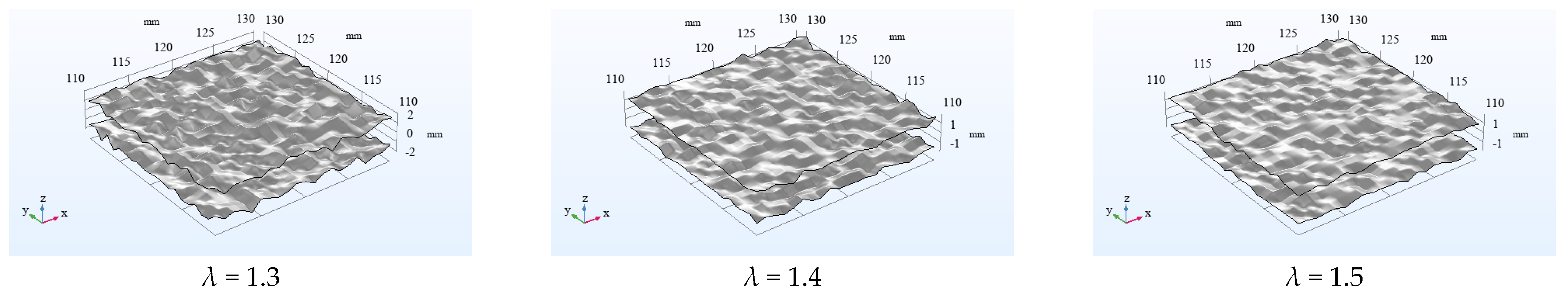
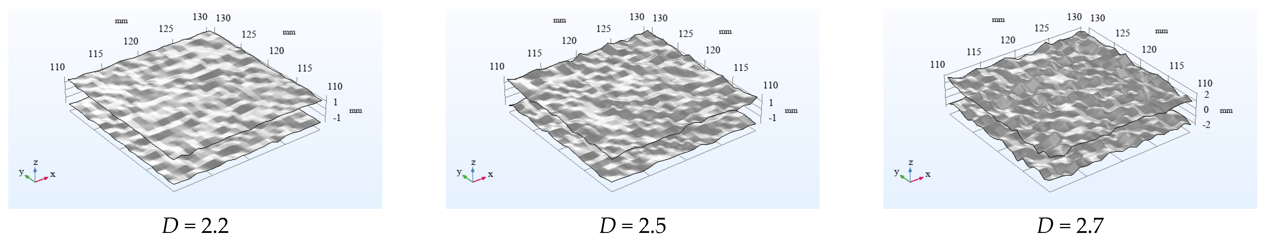
4.2.1. Illustrations on Typical Scenarios of Rough Fracture Surfaces with Varying Different Influencing Factors

By varying specific influencing factors while keeping all other parameters constant, a series of surfaces were generated. In each case, the influencing factor was isolated as the sole variable to ensure other parameters remain unchanged. To provide a clearer depiction of the variation in the rough surface, a cropped section of the original image is presented, focusing on the localized roughness. The surfaces are shown in the following sections.

The maximum and minimum distances between the upper and lower roughness surfaces (d_max and d_min), the range of Z-values on the upper surface (Zu), the range of Z-values on the lower surface (Zl), the relative difference in average aperture (RD_A), average aperture (μ), standard deviation of aperture (σ), and the conformity to normal distribution were statistically analyzed to ascertain the impact of various parameters on roughness. However, the results for the different levels within the same influencing factor showed no significant differences and exhibited similar trends. To enhance data presentation efficiency and simplify table content, the data from the original multiple levels were combined into one comprehensive level, representing the average of the various levels to reflect the overall results. Therefore, the results presented below have been processed and organized in the tables according to this methodology.

The aperture is adjusted vertically by 1.5 mm from the 0-plane, creating rough surfaces on the shifted plane, with all parameters exerting a limited impact on μ. Furthermore, the frequency-distribution composite histograms of the d-values for rough surfaces, derived from varying influencing factors, further validate the influence of parameter variations on fracture surface roughness. Due to space constraints, only the histograms depicting the most prominent effects of parameter variations on the frequency distribution of d-values are presented. Nonetheless, comprehensive analyses of all results are detailed in the respective subsections.

The established relationships between fracture parameters and roughness characteristics hold substantial significance for groundwater modeling applications. The comprehensive sensitivity analysis of these parameters provides critical insights that guide the selection of appropriate scales for incorporating fracture properties into groundwater models while enhancing our understanding of prediction uncertainties arising from fracture roughness variations. Furthermore, this analysis enables computational optimization by identifying and focusing on the most influential parameters (D and λ) in flow simulations.

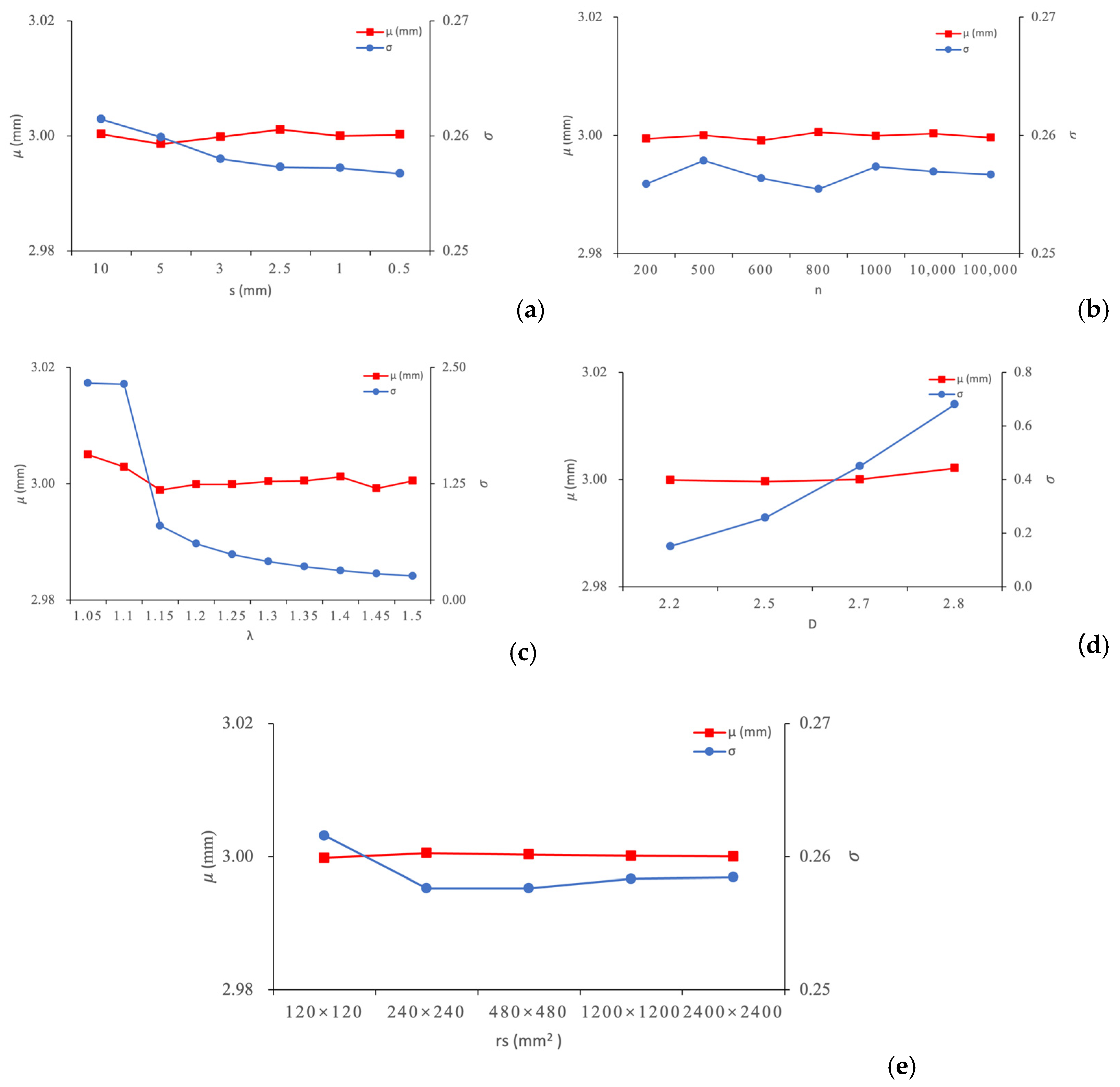
4.2.2. Effect of Segmentation on Roughness

Segmentation indicates the distance between points in the generation of a rough surface. Six levels of this factor are chosen: 10 mm, 5 mm, 3 mm, 2.5 mm, 1 mm, 0.5 mm. In the function model, n = 800, λ = 1.5, D = 2.5, rs = 240 × 240 mm² were determined. The surface images generated at different s values (selecting only s = 10 mm, 3 mm, and 1 mm) are shown in Figure 2.

The specific results are shown in

Table 4. Effects of various parameters on roughness: s, n, λ, D, and rs.

Factor	Value	dmax (mm)	dmin (mm)	Zu (mm)		Zl (mm)		RDA	$\mathit{\mu }$ (mm)	$\mathit{\sigma }$
s (mm)	10	3.71	2.24	1.06	1.93	−1.94	−1.07	0.021%	3.0003	0.2614
	5	3.78	2.22	1.06	1.94	−1.94	−1.06	0.130%	2.9986	0.2599
	3	3.81	2.20	1.06	1.94	−1.94	−1.06	0.053%	2.9998	0.2580
	2.5	3.83	2.18	1.06	1.94	−1.94	−1.06	0.035%	3.0011	0.2573
	1	3.85	2.14	1.06	1.94	−1.94	−1.06	0.002%	3.0000	0.2572
	0.5	3.87	2.14	1.06	1.94	−1.94	1.06	0.001%	3.0002	0.2567
n	200	3.852	2.134	1.06	1.94	−1.94	−1.06	0.057%	2.9994	0.2559
	500	3.849	2.145	1.06	1.94	−1.94	−1.06	0.026%	3.0000	0.2579
	600	3.848	2.147	1.06	1.94	−1.94	−1.06	0.022%	2.9991	0.2564
	800	3.854	2.143	1.06	1.94	−1.94	−1.06	0.019%	3.0005	0.2554
	1000	3.858	2.144	1.06	1.94	−1.94	−1.06	0.011%	2.9999	0.2573
	10,000	3.854	2.153	1.06	1.94	−1.94	−1.06	0.035%	3.0003	0.2569
	100,000	3.857	2.140	1.06	1.94	−1.94	−1.06	0.034%	2.9996	0.2567
λ	1.05	10.79	−4.79	—	—	—	—	0.361%	3.0050	2.3326
	1.1	6.91	−0.95	—	—	—	—	0	3.0029	2.3199
	1.15	5.42	0.47	0.12	2.86	−2.86	−0.12	0.299%	2.9839	0.7973
	1.2	5.01	1.00	0.45	2.55	−2.55	−0.45	0.074%	2.9999	0.6045
	1.25	4.62	1.38	0.65	2.35	−2.35	−0.65	0.095%	2.9999	0.4885
	1.3	4.37	1.63	0.79	2.2	−2.2	−0.79	0.060%	3.0004	0.4136
	1.35	4.19	1.80	0.88	2.12	−2.12	−0.88	0.050%	3.0005	0.3579
	1.4	4.06	1.94	0.95	2.04	−2.04	0.95	0.051%	3.0012	0.3160
	1.45	3.94	2.06	1.01	1.99	−1.99	−1.01	0.016%	2.9992	0.2821
	1.5	3.85	2.13	1.06	1.94	−1.94	−1.06	0.020%	3.0005	0.2574
D	2.2	3.50	2.49	1.24	1.80	−1.76	−1.24	0.021%	2.9999	0.1505
	2.5	3.86	2.14	1.06	1.94	−1.94	−1.06	0.014%	2.9996	0.2568
	2.7	4.50	1.53	0.73	2.27	−2.27	−0.73	0.019%	3.0000	0.4492
	2.8	5.30	0.74	0.32	2.68	−2.68	−0.32	0.053%	3.0021	0.6802
rs (mm2)	$120\times 120$	3.83	2.18	1.06	1.94	−1.94	−1.06	0.037%	2.9998	0.2593
	$240\times 240$	3.85	2.15	1.06	1.94	−1.94	−1.06	0.028%	3.0005	0.2561
	$480\times 480$	3.87	2.13	1.06	1.94	−1.94	−1.06	0.006%	3.0003	0.2561
	$1200\times 1200$	3.88	2.12	1.06	1.94	−1.94	−1.06	0.006%	3.0001	0.2567
	$2400\times 2400$	3.88	2.12	1.06	1.94	−1.94	−1.06	0.002%	3.0000	0.2568

. The results indicate that the Z-values of both the upper and lower surfaces with varying segmentation accuracies follow a normal distribution and exhibit the same range. The distance (d) between the upper and lower rough surfaces is mainly distributed within the range of 2.2 to 3.8 mm.

The parameters μ and σ were identified as key controlling factors and are plotted in Figure 3a, revealing that segmentation accuracy has minimal effect on μ. However, there were finer segmentation results in a smoother distribution of distance values between the upper and lower rough surfaces. When s ≤ 3 mm, σ remains stable. The composite frequency histograms of d-value further substantiating that the stability of the d-value distribution is significantly improved when s ≤ 3 mm.

4.2.3. Effect of Summation Number n on Roughness

This study evaluated seven levels of the function parameter n, specifically: 200, 500, 600, 800, 1000, 10,000, and 100,000. The function model parameters were set to D = 2.5, λ = 1.5, with s = 1 mm and a study scale of 240 × 240 mm². The surface images generated at different n values (selecting only n = 200, 500, and 100,000) are shown in Figure 4.

The results, shown in Table 4, demonstrate that both Zu and Zl at various n values consistently follow a normal distribution with stable ranges. The μ values are approximately 3 mm, while the σ are around 0.26, maintaining stability. For n > 200, the distance (d) between the upper and lower rough surfaces is concentrated between 2.1 and 3.8 mm.

An analysis of the line graph (Figure 3b) for μ and σ reveals that the effect of n on μ is minimal. Furthermore, the composite frequency distribution histograms of d-value at different n values confirm that n > 200 has a negligible effect on roughness.

4.2.4. Effect of λ Parameter on Roughness

This subsection investigates the effect of the parameter λ in the functional equation on surface roughness. Ten levels of λ were selected: 1.05, 1.1, 1.15, 1.2, 1.25, 1.3, 1.35, 1.4, 1.45, and 1.5. The models were set with parameters D = 2.5, n = 800, s = 1 mm, and a study scale of 240 × 240 mm². The surface images generated at different λ values (selecting only λ = 1.3, 1.4, and 1.5) are shown in Figure 5.

The results of this statistical analysis are presented in Table 4. The findings indicate that, irrespective of λ, μ remains largely consistent, while both the Zu and Zl follow a normal distribution. However, a notable difference is observed in the range of d between the upper and lower rough surfaces. When λ is too small, surface penetration occurs, resulting in adherence between the two surfaces at certain locations. For λ exceeding 1.1, no surface penetration is observed. Variations in λ do not significantly alter the overall roughness of the generated surface. Smaller λ values correspond to greater instability in surface roughness undulations.

A line chart of μ and σ (Figure 3c) reveals regular trends in how these metrics vary with different λ values. Specifically, μ varies smoothly, ranging from 2.98 mm to 3.01 mm, with λ exerting a minor effect on μ, resulting in a relatively stable distance. The σ exhibits a distinct trend, becoming flat when λ > 1.15, indicating that the volatility of the distance between the upper and lower surfaces diminishes with increasing λ.

Frequency distribution histograms of d-value for λ values greater than 1.15 is relatively stable. To mitigate the influence of individual outliers or noisy data on the results and improve representativeness, more than 500 points were used to assess the variations in d-value for different λ. For λ = 1.2, the d-value range is 1.8–4.2 mm; for λ = 1.3, it is 2.3–3.7 mm; for λ = 1.4, it is 2.35–3.7 mm; and for λ = 1.5, it is 2.5–3.6 mm. As λ increases to 1.3, the range of d-value narrows significantly. Higher λ values concentrate the distribution of distances on the surface, leading to more consistent geometrical characteristics of the fractures. This demonstrates that larger λ values result in a reduced range of fluctuation in the distances between surfaces, thereby stabilizing the overall geometric features of the surface.

A comprehensive analysis of all graphs indicates that λ affects the stability of surface undulations. Smaller λ values are associated with greater variations in d-value, while λ > 1.15 tends to result in stability. After excluding noisy data, it was observed that for λ ≥ 1.3, λ does not significantly affect the roughness of the fracture.

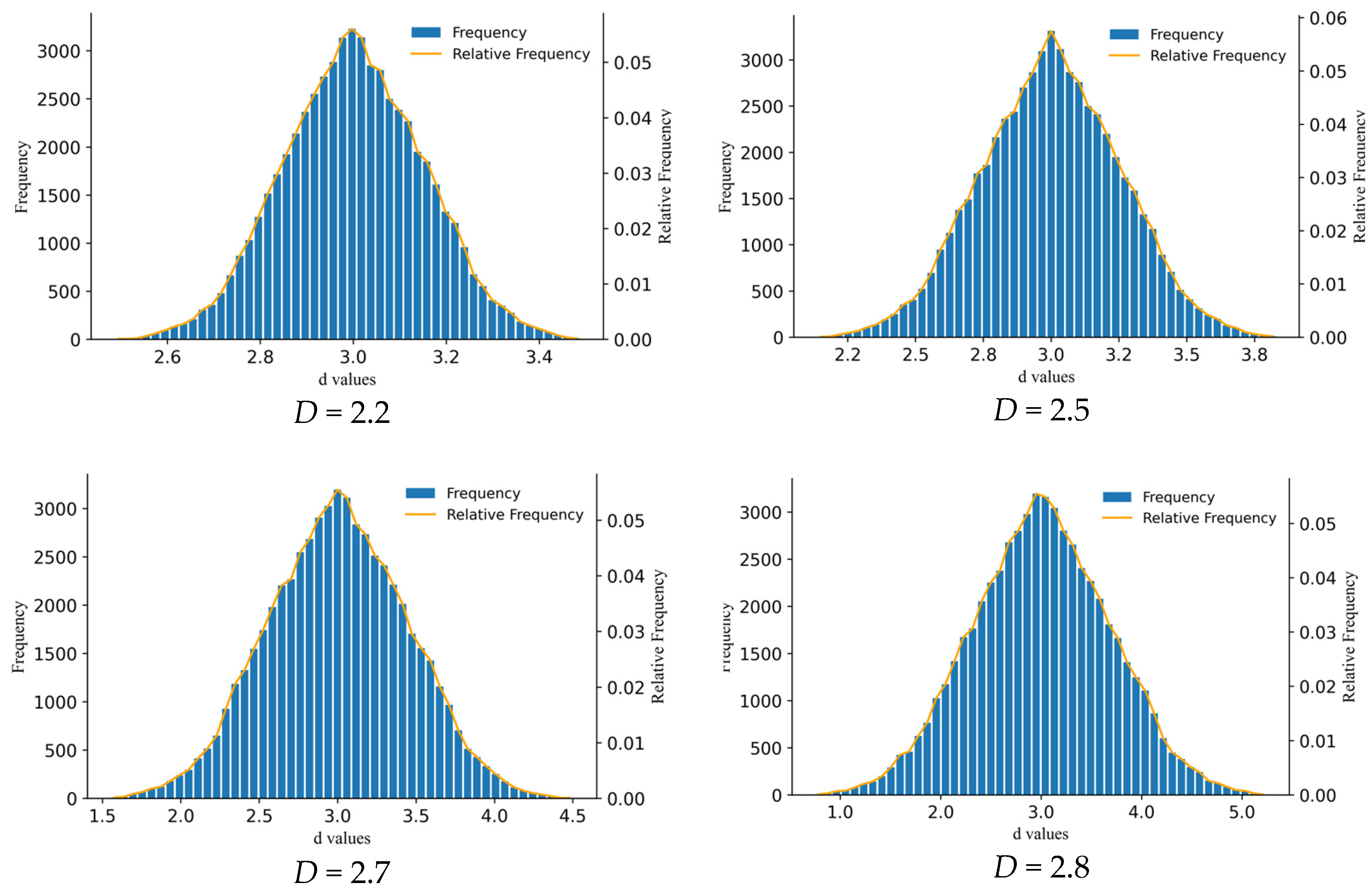
4.2.5. Effect of D Parameter on Roughness

Smooth fracture surfaces have a D value of 2, while rougher and more irregular surfaces have D values between 2 and 3. Four specific D values were selected: 2.2, 2.5, 2.7, and 2.8. For λ = 1.5 and n = 800, with a segmentation accuracy of 1 mm and a scale of 240 × 240 mm². The surface images generated at different D values (selecting only D = 2.2, 2.5, and 2.7) are shown in Figure 6.

Statistical analysis results are shown in Table 4. It is evident that for different D, the range of d between the upper and lower rough surfaces, as well as the range of Z values, differ significantly. However, the Z values for both surfaces adhere to a normal distribution, and μ are essentially the same. The μ and σ were analyzed and plotted as a line graph (Figure 3d) to observe trends across different D. The analysis indicates minimal fluctuation in μ, with values consistently around 3 mm. Conversely, σ increases progressively with D, demonstrating a clear trend: higher D values correspond to greater σ and increased volatility in fracture surface distances.

Frequency histograms provide the most intuitive and clear way to visualize the variation in distances between points on the surface at different D values, revealing extreme values and the distribution of d. This method effectively reduces the influence of extreme values on experimental conclusions, rendering it irreplaceable compared to alternative data processing techniques. Therefore, histograms are essential in this study. Due to the significant impact of D values only their corresponding frequency, histograms are presented in the main text for clarity. Frequency histograms (Figure 7) for distances at various D values show that D significantly impacts fracture surface roughness. Each histogram integrates approximately 60,000 spatially distributed measurements from comprehensive fracture surface analyses, ensuring statistically robust characterizations that effectively mitigate potential distortions from outlier values or instrumental noise. The orange curve delineates the frequency distribution of spacing values (d) across the entire dataset, with distinct fractal dimensions (D) represented by different data series. A detailed analysis of these histograms, based on more than 500 data points, helps mitigate the influence of outliers or noisy data, enhancing result representativeness. For D = 2.2, the d value range is 2.72–3.28 mm; for D = 2.5, it is 2.5–3.5 mm; for D = 2.7, it is 2.15–3.8 mm; and for D = 2.8, it is 1.8–4.4 mm. The variation in d increases with larger D. The analysis reveals a clear positive correlation between fractal dimension and spacing variability. As D increases from lower to higher values, both the total range of d measurements expands and a pronounced clustering of data density near d = 3 mm is observed. This indicates that fractal dimension D exerts significant control over both the spatial distribution patterns and morphological variation characteristics of surface discontinuities. The systematic progression toward higher d values with increasing D provides quantitative evidence that greater fractal complexity corresponds to increased microstructural heterogeneity.

In summary, while μ remains largely unaffected by D, the geometric inhomogeneity within the plane increases with D, leading to greater dispersion in the distances between points. This suggests that D significantly influences surface roughness; higher D values correlate with increased microstructural differences and greater surface roughness.

4.2.6. Effect of Investigation Sizes on Roughness

To investigate the scale effect of the surface method and assess the representativeness of the study ranges, five different study ranges were selected: 120 × 120; 240 × 240; 480 × 480; 1200 × 1200; and 2400 × 2400 mm². For λ = 1.5, n = 800, D = 2.5, and s = 1 mm. The surface images generated at different rs values (selecting only rs = 120 × 120 mm², 240 × 240 mm², and 1200 × 1200 mm²) are shown in Figure 8.

The specific results are presented in Table 4. The results show that under different rs, the Z values of the upper and lower surfaces consistently conform to a normal distribution with a similar range of variation. The d values are maintained between 2.15 and 3.9 mm, with μ for the upper and lower roughness surfaces approximately equal to 3. σ is approximately 0.26. Figure 3e, plotting μ and σ, demonstrates that there is no significant variation in the surface roughness characteristics for rs ≥ 240 × 240 mm², indicating that the roughness of the surface becomes negligible beyond the threshold. Furthermore, the frequency distribution histograms of the d-value at different rs similarly shows that the roughness remains largely unaffected for rs ≥ 240 × 240 mm². It is a representative size for characterizing the considered fracture roughness.

4.3. Regression Models for Impacts of Multiple Parameters on Roughness

This study constructs a statistical prediction model for σ₁ based on the orthogonal experimental design outlined in Table 2. The independent variables (X) include D, λ, n, and s, while the dependent variable (Y) is the standard deviation of the aperture (σ). The multiple regression analyses were conducted using SPSS software (v22) and the following regression equation was obtained.

$${\sigma }_1={\mathrm{e}}^{-4.886}\times s^{-0.0048}\times n^{-0.0099}\times {\lambda }^{-3.995}\times D^{5.693}.$$

(8)

The R² value of Equation (8) was found to be 0.9669, demonstrating a good model fit. In Equation (8) D and λ exhibited the largest positive and negative effects on σ, respectively. A new regression relationship between the two primary controlling factors and σ was established as follows.

$${\mathsf{\sigma }}_2={\mathrm{e}}^{-4.828}\times {\lambda }^{-3.995}\times D^{5.693}.$$

(9)

The R² value of Equation (9) was determined to be 0.9667, demonstrating a well-fitted model. All validation data presented in Table 1 were incorporated into Equations (8) and (9) to verify their accuracy. Data grouping was performed using categorical averaging to minimize redundancy, resulting in a total of 21 datasets that present the predicted values from different regression equations (${\sigma }_1^{’},{\sigma }_2^{’}),$ along with the corresponding Relative Prediction Errors (RPE₁ and RPE₂). The graphs are shown in Figure 9.

An analysis of the results reveals that the standard deviation values obtained after validating the regression Equation (8) are consistently lower than those for Equation (9). An analysis of the results shows that the validation outcomes for both Equations (8) and (9) remained stable at approximately 0.3 for the first twelve sequences. Starting with the thirteenth sequence, both equations exhibited a significant increase in validation results, with Equation (9) demonstrating a more pronounced rise. After reaching a peak, the results declined until the eighteenth sequence. From the nineteenth to the twenty-first sequence, the validation results for both equations began to increase again. The sequences from thirteenth to eighteenth correspond to validation results for changes in λ (1.2–1.45), while the nineteenth to the twenty-first sequences correspond to changes in D (2.2, 2.7, 2.8). This indicates that D and λ significantly affect the roughness of the fracture.

In the first eighteen sequences, RPE₁ is significantly smaller than RPE₂, especially in the first eleven sequences, where RPE₁ remains below 3%. RPE₁ reaches its maximum value at the twenty-first sequence, while RPE₂ peaks at the fifteenth sequence, reinforcing the observation that D and λ influence the roughness of the fracture positively and negatively, respectively. Equation (9), which considers only two key factors, still achieves similar performance in predicting the effects of D and λ on fracture roughness. Overall, Equation (8) demonstrates superior predictive performance compared to Equation (9).

In this section, a qualitative analysis is conducted on the effects of five parameters—D, λ, n, s, and rs—on the roughness of the fracture surface. The results indicated that both D and λ significantly affect surface roughness, while the other parameters have a lesser impact. Furthermore, the effect of D is more pronounced than that of λ. The effects of D and λ on roughness were then quantitatively investigated by using D, λ, n, and s as the independent variables (X) and σ as the dependent variable (Y), followed by an analysis of principal control factors. To verify the accuracy of model, the aforementioned experimental results were compared and analyzed, revealing significant agreement between the actual effects of D and λ and the model predictions, thereby confirming that D and λ are key factors affecting roughness. The influence of D on roughness is particularly prominent, while λ also exhibits some influence, albeit weaker than D. When λ ≥ 1.3, D predominantly controlled fracture roughness.

4.4. Examinations on Impacts of Different Parameters by 3D-Printed Rough Fracture Experiments and Numerical Simulations

The rough fracture surface generated under these parameters serves as a representative fracture surface for laboratory-scale rock equipment. This representation is based on the significant effects of D and λ on roughness observed in previous studies, particularly when s ≤ 3 mm, n > 200, λ ≥ 1.3, and rs ≥ 240 × 240 mm². In this section, hydrodynamic experiments are conducted using the printed physical device, alongside corresponding numerical simulations, to assess the effects of parameters s, n, λ, D, and rs on roughness, thereby validating the representativeness of the laboratory-scale fracture surface within the specified parameter ranges.

Hydrodynamic experiments were performed under saturated conditions, involving three sets of experiments where the inlet serves as the head boundary and the outlet served as the flow boundary. The physical experiments were conducted under controlled conditions: ambient temperature (20 ± 1 °C), atmospheric pressure (101 ± 1 kPa), relative humidity (35–45%), along with proper instrument calibration. The water temperature was maintained at a constant (20 ± 1 °C) throughout the experiment. Scale markers were placed at various locations on the experimental setup to facilitate accurate readings of the inlet and outlet head changes. Once the saturated condition stabilized, head values (h_in, h_out) at both the inlet and outlet, as well as the stable flow rate (q), were recorded. Identical numerical simulations were conducted using COMSOL (v6.1). For the initial conditions, the fracture domain is set to be fully water-saturated, with the water volume fraction V_w set to 1. The surface roughness is generated using the W-M function and the rough fracture is imported into COMSOL to represent the physical fracture surface. For the boundary conditions, the inlet is modeled as a head boundary, consistent with the experimental setup. The water head values at the inlet (h_in) for three different scenarios are set to 19.1 mm, 20.2 mm, and 23.2 mm, respectively. The outlet is set as a constant flow rate (q) boundary to match the experimental flow conditions. The flow rate at the outlet is defined for each of the three different scenarios, ensuring the simulation replicates the experimental conditions. After stabilization, the water head at the outlet (h_out) is measured and compared to the experimental results for validation. The comparison of experimental results (ER) and simulation results (ES) is summarized in

Table 5. Comparison of physical experiment and simulation outcomes across various scenarios.

	Factors	ER	ES	S1	S2	S3	S4	S5	S6	S7
(1)	hin (mm)	19.1
	hout (mm)	17	17.049	17	17.03	17.013	17.360	17.049	17.059	17.061
	q (mL/s)	0.51
	dif		0.288%	−0.29%	−0.11%	−0.21%	1.82%	0.00%	0.06%	0.07%
(2)	hin (mm)	20.2
	hout (mm)	17	17.079	17.025	16.997	16.933	18.089	17.078	17.086	17.094
	q (mL/s)	1.36
	dif		0.465%	−0.58%	−0.48%	−0.86%	5.91%	−0.01%	0.04%	0.09%
(3)	hin (mm)	23.2
	hout (mm)	17	16.927	16.755	16.743	16.673	18.216	16.877	16.960	16.99
	q (mL/s)	2.65
	dif		1.012%	−1.02%	−1.09%	−1.50%	7.62%	−0.30%	0.20%	0.37%

.

The analysis revealed minimal errors between simulation and experimental results, with simulation accuracy generally exceeding 99%. These findings indicate that the simulation results are reliable representations of the physical experiments. Based on these results, additional simulation scenarios were constructed to further explore the effects of various parameters on fracture roughness and to verify the representativeness of the laboratory-scale fracture surface. Different numerical simulations were constructed in COMSOL, with the inlet set as the head boundary and the outlet as the flow boundary. Water flow simulations under saturated conditions were performed across three different initial conditions, reflecting the experimental scenarios. The specific simulation scenarios are detailed in Table 3. The deviations between ES and new simulation results are also shown in Table 5.

Among the seven sets of simulation results, most scenarios exhibited small errors in h_out, with deviations generally below 1%. Notably, Scenarios 5, 6, and 7 displayed negligible errors. Conversely, some scenarios, such as Scenario 3 and Scenario 4, showed relatively large errors, particularly under group (2) conditions, with deviations of −0.86% for Scenario 3 and up to 5.914% for Scenario 4. These discrepancies indicate that D has a significant effect on surface roughness, while λ also influences roughness, with the error associated with D being approximately seven times greater than that of λ. Higher flow rates corresponded to greater deviations between simulation results and physical experiments. In this study, a set of representative parameters (s = 3mm, n = 800, λ = 1.5, D = 2.7, rs = 240 mm) was selected to design the experimental setup for conducting relevant hydraulic experiments. Based on these experiments, numerical simulations were performed to examine the effects of different parameters on fracture roughness. During the physical experiments, the measurement precision was maintained at 0.1mm; however, future studies could utilize higher-precision instrumentation to further enhance experimental accuracy. Although the most representative experimental setup was adopted, additional experimental setups could be designed to expand the analysis scope. For example, when D is smaller (D = 2.3), the fracture surface becomes smoother, and comparative experiments under identical hydraulic conditions could reveal roughness variations. While s ≤ 3mm has been shown to exert negligible influence on roughness, future investigations could explore smaller s values (s = 1 mm) to further assess their potential impact. These improvements would enhance experimental reliability and broaden the applicability of the findings, providing a robust foundation for generalized fracture roughness characterization. Further research is necessary to investigate the mechanisms of seepage effects under varying flow velocities in rough fractures.

Overall, the results of this section align with the findings of previous sections, reaffirming that both D and λ significantly influence the surface characteristics of rough fractures, while other parameters have less influence. The surface characteristics of rough fractures tend to stabilize when using the representative parameters of n > 200 and λ ≥ 1.3, alongside s ≤ 3 mm and rs = 240 × 240 mm² for the rough surface model in the laboratory. This means that under the conditions of s ≤ 3 mm, n > 200, λ ≥ 1.3, and rs ≥ 240 × 240 mm², roughness can be controlled by adjusting the variations in D.

These findings significantly enhance our ability to characterize fracture properties in regional groundwater models, thereby improving the accuracy of subsurface flow predictions. The framework not only refines the assessment of model uncertainties but also provides valuable insights into scale-dependent effects and optimization of model parameterization. Furthermore, the methodology developed in this study demonstrates substantial potential for integration with emerging machine learning techniques, offering a robust foundation for advancing predictive capabilities in groundwater modeling and supporting the sustainable management of large-scale groundwater resources.

5. Conclusions

Through statistical analysis, experimental verification, and numerical simulation, this study integrates fractal analyses with 3D printing technology to develop a practical framework for generating accurate and controllable rock fracture roughness. This advancement improves the accuracy and interpretability of experimental results. The key conclusions are presented as follows:

(1)

Based on the datasets of the rough surfaces of rock fractures generated using the 3D Weierstrass–Mandelbrot (W-M) approach, a univariate analysis of five factors including fractal dimension D, frequency density factor λ, segmentation accuracy s, summation number n, and investigation scale rs was conducted. It was found that s and n have a minor impact on roughness, exhibiting negligible effects when s ≤ 3 mm and n > 200. However, λ and D significantly affect the geometric heterogeneity of the fracture surface, while roughness remains largely unchanged when λ ≥ 1.3. When rs ≥ 240 × 240 mm², fracture roughness does not significantly change with increases in rs, indicating a representative size for characterizing the considered fracture roughness.

(2)

With the representative investigation size of rs being 240 × 240 mm², D, λ, n, and s were selected as controlling parameters using an orthogonal experimental design to generate representative fracture surface data. Based on these data, two multiple regression statistical models were established correlating aperture standard deviation σ with all influencing factors (D, λ, n, and s) and with the two key controlling factors (D and λ). Both models demonstrated excellent fitting (R² = 0.97). When λ ≥ 1.3, D predominantly controls fracture roughness, consistent with the findings from the univariate analysis. The verification results confirm the reliability of these regression models.

(3)

The laboratory-scale rough rock specimens were generated using 3D printing technology under the conditions of s ≤ 3 mm, n > 200, λ ≥ 1.3, and rs ≥ 240 × 240 mm². These samples facilitated hydrodynamic experimentation under saturated conditions. Empirical data confirmed the accuracy and reliability of numerical simulations, indicating that the constructed models effectively represent physical experiments. The groundwater flow simulations based on the physical model, in which these influencing factors s, n, λ, and D have been accounted for, demonstrated consistency with prior statistical analyses. It has been validated that s and n minimally effect roughness, particularly when s ≤ 3 mm and n > 200. In contrast, D and lower λ significantly affect the geometric heterogeneity of the fracture surface. The roughness can be controlled by D under the conditions of s ≤ 3 mm, n > 200, λ ≥ 1.3, and rs ≥ 240 × 240 mm². This parametric sensitivity analysis empowers technicians to efficiently control surface roughness through the calibration of parameter D under the specified constraints, enabling precise replication of target conditions.

(4)

This study lays the foundation for accurately characterizing rough fracture surfaces and effectively constructing relevant experimental devices, providing technicians with a reliable approach for generating consistent rough fractures using the W-M method. The validated roughness characterization methodology enables a more accurate representation of fracture properties in groundwater models, improving the prediction accuracy of groundwater flow and contaminant transport in fractured aquifers, supporting more effective groundwater utilization and management. Specifically, an effective framework has been presented as a reference for various experimental and numerical investigations, along with practical applications such as groundwater seepage, solute transport, and multiphase flow including migrations of contaminants or petroleum NAPLs in rough fractures of fractured rocks. Despite its achievements, this study is limited to single-phase flow under laboratory conditions. Future research should focus on three key areas: (1) multiphase flow dynamics in rough fractures, especially gas–water or NAPL–water interactions relevant to contaminated aquifer remediation; (2) coupled thermo-hydro-mechanical-chemical processes, including mineral dissolution/precipitation that affect fracture morphology over time; and (3) the development of upscaling methods to apply laboratory results to field-scale fractured aquifer systems. Additionally, the W-M method could be extended to characterize fracture networks, improving our understanding of flow and transport in complex fractured media at watershed scales.

References

1. Dou, Z.; Sleep, B.; Zhan, H.; Zhou, Z.; Wang, J. Multiscale Roughness Influence on Conservative Solute Transport in Self-Affine Fractures. Int. J. Heat Mass Transf. 2019, 133, 606–618. [Google Scholar] [CrossRef]
2. Zou, L.; Jing, L.; Cvetkovic, V. Modeling of Flow and Mixing in 3D Rough-Walled Rock Fracture Intersections. Adv. Water Resour. 2017, 107, 1–9. [Google Scholar] [CrossRef]
3. Zhang, Y.; Ye, J.; Li, P. Flow Characteristics in a 3D-Printed Rough Fracture. Rock Mech. Rock Eng. 2022, 55, 4329–4349. [Google Scholar] [CrossRef]
4. Zandarin, M.T.; Alonso, E.; Olivella, S. A Constitutive Law for Rock Joints Considering the Effects of Suction and Roughness on Strength Parameters. Int. J. Rock Mech. Min. Sci. 2013, 60, 333–344. [Google Scholar] [CrossRef]
5. Azinfar, M.J.; Ghazvinian, A.H.; Nejati, H.R. Assessment of Scale Effect on 3D Roughness Parameters of Fracture Surfaces. Eur. J. Environ. Civ. Eng. 2019, 23, 1–28. [Google Scholar] [CrossRef]
6. Alberti, L.; Antelmi, M.; Oberto, G.; La Licata, I.; Mazzon, P. Evaluation of Fresh Groundwater Lens Volume and Its Possible Use in Nauru Island. Water 2022, 14, 3201. [Google Scholar] [CrossRef]
7. Song, Z.; Wang, Y.; Wang, J.; Huan, H.; Li, H. Design of Pump-and-Treat Strategies for Contaminated Groundwater Remediation Using Numerical Modeling: A Case Study. Water 2024, 16, 3665. [Google Scholar] [CrossRef]
8. Brinksmeier, E.; Riemer, O. Measurement of Optical Surfaces Generated by Diamond Turning. Int. J. Mach. Tools Manuf. 1998, 38, 699–705. [Google Scholar] [CrossRef]
9. Deng, H.; Fitts, J.P.; Peters, C.A. Quantifying Fracture Geometry with X-Ray Tomography: Technique of Iterative Local Thresholding (TILT) for 3D Image Segmentation. Comput. Geosci. 2016, 20, 231–244. [Google Scholar] [CrossRef]
10. Tian, Z.; Dai, C.; Zhao, Q.; Meng, Z.; Zhang, B. Experimental Study of Joint Roughness Influence on Fractured Rock Mass Seepage. Geofluids 2021, 2021, 8813743. [Google Scholar] [CrossRef]
11. Phillips, T.; Bultreys, T.; Bisdom, K.; Kampman, N.; Offenwert, S.; Mascini, A.; Cnudde, V.; Busch, A. A Systematic Investigation Into the Control of Roughness on the Flow Properties of 3D-Printed Fractures. Water Resour. Res. 2021, 57, 25233. [Google Scholar] [CrossRef]
12. Zhu, C.; Xu, X.; Wang, X.; Xiong, F.; Tao, Z.; Lin, Y.; Chen, J. Experimental Investigation on Nonlinear Flow Anisotropy Behavior in Fracture Media. Geofluids 2019, 2019, 5874849. [Google Scholar] [CrossRef]
13. Cui, W.; Wang, L.; Luo, Y. Modeling of Three-Dimensional Single Rough Rock Fissures: A Study on Flow Rate and Fractal Parameters Using the Weierstrass-Mandelbrot Function. Comput. Geotech. 2022, 144, 104655. [Google Scholar] [CrossRef]
14. Develi, K.; Babadagli, T. Quantification of Natural Fracture Surfaces Using Fractal Geometry. Math. Geol. 1998, 30, 971–998. [Google Scholar] [CrossRef]
15. Chen, S.J.; Zhu, W.C.; Yu, Q.L.; Liu, X.G. Characterization of Anisotropy of Joint Surface Roughness and Aperture by Variogram Approach Based on Digital Image Processing Technique. Rock Mech. Rock Eng. 2016, 49, 855–876. [Google Scholar] [CrossRef]
16. Ju, Y.; Ren, Z.; Zheng, J.; Gao, F.; Mao, L.; Chiang, F.; Xie, H. Quantitative Visualization Methods for Continuous Evolution of Three-Dimensional Discontinuous Structures and Stress Field in Subsurface Rock Mass Induced by Excavation and Construction—An Overview. Eng. Geol. 2020, 265, 105443. [Google Scholar] [CrossRef]
17. Chen, Y.; Liang, W.; Lian, H.; Yang, J.; Nguyen, V.P. Experimental Study on the Effect of Fracture Geometric Characteristics on the Permeability in Deformable Rough-Walled Fractures. Int. J. Rock Mech. Min. Sci. 2017, 98, 121–140. [Google Scholar] [CrossRef]
18. Zhang, X.; Jiang, Q.; Chen, N.; Wei, W.; Feng, X. Laboratory Investigation on Shear Behavior of Rock Joints and a New Peak Shear Strength Criterion. Rock Mech. Rock Eng. 2016, 49, 3495–3512. [Google Scholar] [CrossRef]
19. Ge, Y.; Kulatilake, P.H.S.W.; Tang, H.; Xiong, C. Investigation of Natural Rock Joint Roughness. Comput. Geotech. 2014, 55, 290–305. [Google Scholar] [CrossRef]
20. Kou, M.; Liu, X.; Tang, S.; Wang, Y. Experimental Study of the Prepeak Cyclic Shear Mechanical Behaviors of Artificial Rock Joints with Multiscale Asperities. Soil Dyn. Earthq. Eng. 2019, 120, 58–74. [Google Scholar] [CrossRef]
21. Ishibashi, T.; Fang, Y.; Elsworth, D.; Watanabe, N.; Asanuma, H. Hydromechanical Properties of 3D Printed Fractures with Controlled Surface Roughness: Insights into Shear-Permeability Coupling Processes. Int. J. Rock Mech. Min. Sci. 2020, 128, 104271. [Google Scholar] [CrossRef]
22. Mecholsky, J.J.; Passoja, D.E.; Feinberg-Ringel, K.S. Quantitative Analysis of Brittle Fracture Surfaces Using Fractal Geometry. J. Am. Ceram. Soc. 1989, 72, 60–65. [Google Scholar] [CrossRef]
23. Rong, G.; Cheng, L.; He, R.; Quan, J.; Tan, J. Investigation of Critical Non-Linear Flow Behavior for Fractures with Different Degrees of Fractal Roughness. Comput. Geotech. 2021, 133, 104065. [Google Scholar] [CrossRef]
24. Datseris, G.; Kottlarz, I.; Braun, A.P.; Parlitz, U. Estimating Fractal Dimensions: A Comparative Review and Open Source Implementations. Chaos Interdiscip. J. Nonlinear Sci. 2023, 33, 102101. [Google Scholar] [CrossRef]
25. Li, G.; Zhang, K.; Gong, J.; Jin, X. Calculation Method for Fractal Characteristics of Machining Topography Surface Based on Wavelet Transform. Procedia CIRP 2019, 79, 500–504. [Google Scholar] [CrossRef]
26. Zhang, X.; Xu, Y.; Jackson, R.L. An Analysis of Generated Fractal and Measured Rough Surfaces in Regards to Their Multi-Scale Structure and Fractal Dimension. Tribol. Int. 2017, 105, 94–101. [Google Scholar] [CrossRef]
27. Ju, Y.; Zhang, Q.; Yang, Y.; Xie, H.; Gao, F.; Wang, H. An Experimental Investigation on the Mechanism of Fluid Flow through Single Rough Fracture of Rock. Sci. China Technol. Sci. 2013, 56, 2070–2080. [Google Scholar] [CrossRef]
28. Jinguo, W.; Zhifang, Z. Simulation of Coupled Fluid Flow and Solute Transport in a Rough Fracture. In Elsevier Geo-Engineering Book Series; Stephanson, O., Ed.; Elsevier: Berlin/Heidelberg, Germany, 2004; Volume 2, pp. 565–570. ISBN 1571-9960. [Google Scholar]
29. Li, N.; Yang, X.; Zhang, P. Numerical Simulation of the Morphology and the Geometric Characteristic of Rock Joints by Using GIS; CRC Press: Boca Raton, FL, USA, 2008. [Google Scholar]
30. Yan, W.; Komvopoulos, K. Contact Analysis of Elastic-Plastic Fractal Surfaces. J. Appl. Phys. 1998, 84, 3617–3624. [Google Scholar] [CrossRef]
Figure 1. Images of experimental setups.
Water 17 00982 g001
Figure 2. Rough fracture surfaces generated under various s.
Water 17 00982 g002
Figure 3. Comparative analyses of μ, σ under various conditions: (a) Comparison of μ and σ for various s values. (b) Comparison of μ and σ for various n values. (c) Comparison of μ and σ for various λ values. (d) Comparison of μ and σ for various D values. (e) Comparison of μ and σ at various rs.
Water 17 00982 g003
Figure 4. Rough fracture surfaces generated under various n.
Water 17 00982 g004
Figure 5. Rough fracture surfaces generated under various λ.
Water 17 00982 g005
Figure 6. Rough fracture surfaces generated under various D.
Water 17 00982 g006
Figure 7. Histograms of d-value frequency distribution for various D values.
Water 17 00982 g007
Figure 8. Rough fracture surfaces generated under various rs.
Water 17 00982 g008
Figure 9. Comparison of σ 1 , σ 2 , RPE1, and RPE2.
Water 17 00982 g009