Influence of Precipitation on the Estimation of Karstic Water Storage Variation

Abstract

Karst water supplies freshwater to approximately a quarter of the global population and plays a crucial role in supporting the socioeconomic development of karst regions. As a key indicator for assessing and managing karst water resources, karstic water storage variation is influenced not only by the complex structure of karst aquifer media but also by the variability in natural precipitation infiltration. Based on the hydrogeological conditions of a typical karst aquifer system in northern China, this study developed a three-dimensional physical experimental setup and established a corresponding groundwater flow numerical model coupled with equivalent porous media and conduits. The factors affecting spring flow recession were investigated from a source–sink perspective. Precipitation events were categorized into two types: those with the same duration but different intensities and those with the same total volume but different intensities. The influence of varying precipitation events on the estimation of karstic water storage variation was quantitatively evaluated using the exponential fitting method, based on the analysis of spring flow recession curves. These findings could provide scientific guidance for the development, utilization, and protection of karst water resources.

1. Introduction

The abundant groundwater resources in karst regions are crucial for local production and daily life. However, the uneven spatial distribution of karst aquifer media complicates the understanding of groundwater occurrence patterns, making it difficult to precisely estimate karstic water storage variation (KWSV). This complexity presents significant obstacles in the exploitation and utilization of karst water resources [1,2]. KWSV represents the volume of groundwater that can be stored and discharged during a specific period. It is a crucial parameter in assessing and managing groundwater resources. An accurate estimation of KWSV offers valuable insights into the sustainability and availability of karst water, which is vital for efficient groundwater management and strategic planning [3].

The accurate calculation of KWSV often presents certain difficulties and requires careful consideration in selecting appropriate calculation methods. Currently, scholars have proposed several methods for estimating KWSV, each with its own advantages and limitations. (1) Geometric evaluation methods based on porosity [4,5]. Estimating effective porosity in karst aquifer systems is crucial when applying this method. However, due to the high heterogeneity of karst aquifer media, obtaining these data can be challenging and costly. (2) Tracer method. This method can estimate the water volume stored and discharged in aquifers by measuring the concentration changes in tracers over time. However, it requires long-term time-series of stable isotope relative abundances, which are often difficult to obtain and unsuitable for many practical situations [6,7]. (3) Numerical simulation method. The use of numerical models necessitates a large amount of detailed hydrogeological data, which are often difficult to obtain in karst regions [8,9]. (4) Exponential equation fitting method based on spring flow recession curve analysis. This widely used method estimates KWSV [10,11,12] by analyzing the complete spring flow recession process over time after a rainy or recharge event. It is relatively simple and economically efficient. For situations where other methods cannot obtain data, the exponential equation fitting method based on spring flow recession curve analysis is the most attractive.

The KWSV is not only controlled by the complex structure of karst aquifer media but is also influenced by variable natural and artificial recharge, runoff, and discharge conditions [13,14,15]. Among them, the structure of the karst aquifer and various precipitation events play a significant role in shaping the spring flow recession curve, which in turn impacts the accuracy of KWSV estimation. For the impact of karst aquifer structures on karst water dynamics, scholars have conducted extensive research. For example, two key hydrogeological parameters of the karst matrix—hydraulic conductivity and specific yield—both influence the shape and recession coefficient of this curve [16]. The hydraulic conductivity is an indicator of the groundwater transport capacity of a karst matrix under a hydraulic gradient [17]. Higher hydraulic conductivity indicates faster groundwater movement through the karst matrix, potentially leading to a steeper recession curve. In contrast, specific yield indicates the volume of groundwater that can be discharged from the matrix under the influence of gravity [18]. A higher specific yield allows for greater groundwater discharge, requiring more time for the aquifer to fully deplete, which may result in a smoother recession curve. Many scholars, both home and abroad, have conducted relevant research. For example, Abirifard et al. [19] conducted numerical simulations of groundwater flow in a hypothetical karst aquifer to evaluate the deviation between extrapolated and measured recession curves where they determined the parameters that control the extrapolated recession coefficient, and they reported that as the saturation thickness increases, the increases in high hydraulic conductivity and specific yield lead to an underestimation of the KWSV. Shu et al. [20] created a two-dimensional water tank model along with numerical models (MODLOW-2005, CFPM1) to investigate how fracture hydraulic conductivity affects water exchange between the conduit and the matrix. Their findings suggested that an increase in fracture hydraulic conductivity expands the movement range of groundwater but reduces the water exchange between the conduit and the matrix. In addition, the internal structure of karst conduits also controls the flow behavior of karst water and the spring flow variation, affecting the estimation accuracy of the KWSV. Many scholars have conducted relevant research on karst conduit structures. For example, Chang [21] used the MODFLOW-CFP model to discuss the changes in average and local conduit diameters, as well as the influence of the flow state inside the conduit on karst spring flow rate changes. Peterson [22] evaluated the role of conduit geometry and hydraulic parameters in controlling the internal movement mechanics of karst aquifers by simulating gradual changes in these factors. For the impact of precipitation events on karst water dynamics, scholars have conducted certain research. For example, Abirifard et al. [19] examined the reliability of extrapolating observed spring hydrograph recessions using flow models of hypothetical karst aquifers. The results indicated that parameters like catchment geometry and point recharge have minimal impact on the accuracy of estimated dynamic water volumes. To delve into the impacts of varying precipitation intensities, multi-stage conduit arrangements, and multiple precipitation events on the interaction process between the karst aquifer and the stream, Huang et al. [23] employed the multiphase Darcy–Brinkman–Stokes equation to analyze the interaction process between the karst aquifer and the stream. The results showed that as the intensity of precipitation increases, the interaction process between the karst aquifer and the stream becomes more complex. Mohammadi and Shoja [24] studied the effect of annual precipitation amount on the characteristics of a spring hydrograph such as the recession coefficient, volume of dynamic flow, base flow, and quick flow in two karst springs in Iran. The research results indicated that the hydrodynamic characteristics of a spring hydrograph are controlled by the type of recharge, type of storage, and mechanism of water movement in the karst aquifer. Chang et al. [25] investigated the responses of spring discharge to rainfall events by the continuous monitoring of spring discharge and temperature at a single-conduit karst system. The spring recession processes were analyzed after a series of precipitation events, and the reasons for the change in water recession regular patterns are discussed under different rainfall conditions.

The above studies focused primarily on the influence of the karst aquifer medium structure on the estimation of the KWSV and the influence of precipitation on spring discharge. However, atmospheric precipitation, as the most important source and sink term in karst aquifer systems, directly affects the recharge of karst water. Additionally, various types of precipitation can have a substantial impact on the spring flow recession process, thereby influencing the accuracy of KWSV estimation. Thus, the main objective of this study is to investigate the impact of different precipitation events on the KWSV estimation. To achieve this goal, an equivalent medium–conduit coupled groundwater flow numerical model was developed, based on the hydrogeological conceptual model of a typical karst aquifer system in northern China. Precipitation events are categorized into two types based on common natural precipitation patterns: (1) events with the same duration but different intensities and (2) events with the same total volume but varying intensities. This study aims to quantitatively analyze the influence of different precipitation events on the estimation of the KWSV. The results of this study can provide valuable reference data for the evaluation of karst water resources.

2. Materials and Methods

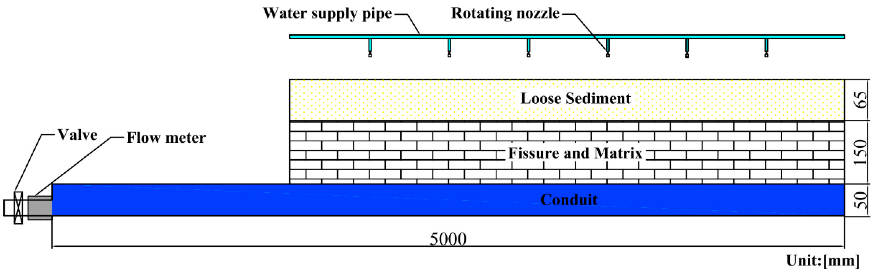
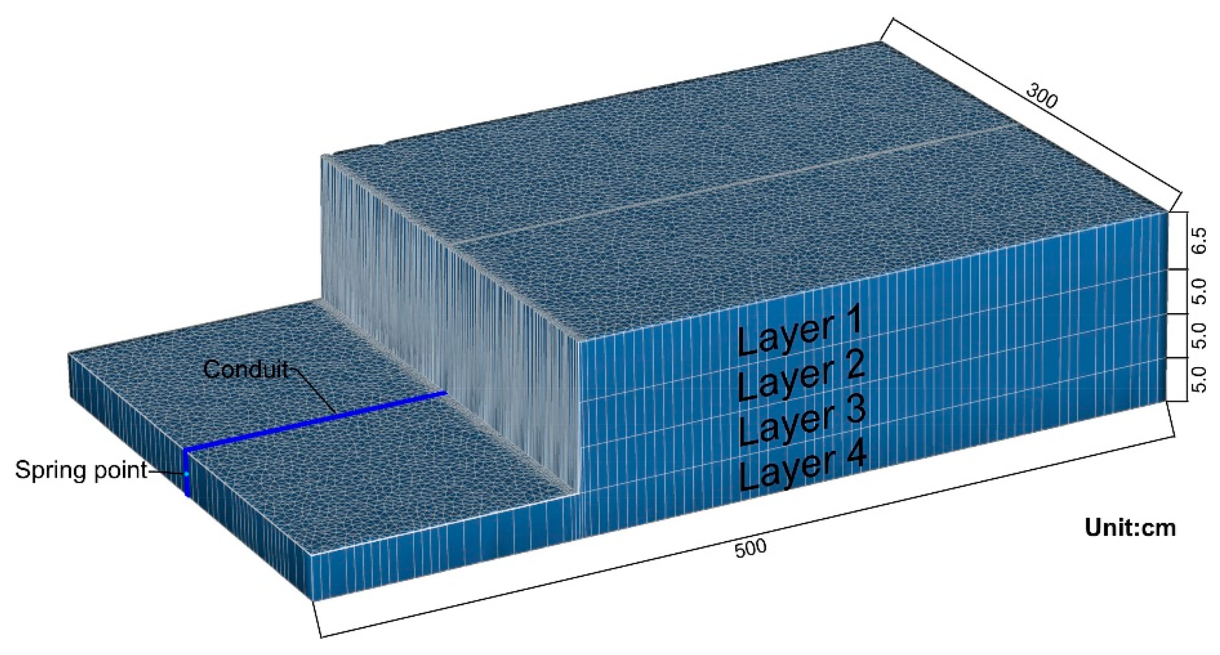
2.1. Construction of the Combined Discrete-Continuum Model

In the covered karst regions of northern China, the karst aquifer is typically located beneath a layer of quaternary loose sediments. The aquifer medium mainly consists of interconnected conduits with high permeability, large fractures, and small fractures that have low permeability. The entire aquifer system is interconnected, with groundwater ultimately being discharged in the form of karst springs or underground rivers. In this study, the hydrogeological characteristics of a typical karst region in northern China were generalized to develop a simplified hydrogeological conceptual model. Additionally, a physical experimental setup was also established, as shown in Figure 1 [26]. In the physical model, the karst aquifer medium is predominantly characterized by a conduit fracture-matrix structure. The loose sediment and karst aquifer media collectively form the main aquifer medium.

Due to the limitations of parameter adjustments in physical experiments and the high cost of repeated tests, it is challenging to meet the diverse parameter settings required for subsequent simulation scenarios. In this study, a numerical model coupling equivalent porous media and conduit groundwater flow was developed to match the physical model. The numerical model was calibrated and validated using groundwater level and spring flow data obtained from the physical experiments as fitting targets. The simulated values of the calibrated and validated numerical model showed good agreement with the measured values from the physical experiments, meeting the error requirements. Therefore, the established numerical model can effectively simulate the groundwater flow processes observed in the indoor physical experiments, enabling further scenario-based simulation analyses. The hydrogeological parameters of the numerical model are shown in

Table 1. Initial settings of the hydrogeological parameters of the groundwater flow numerical model.

Hydrogeological Parameters	Matrix		Conduit
	Hydraulic Conductivity (m/s)	Specific Yield	$\mathbf{Roughness}\mathbf{Coefficient}({\mathbf{m}}^{1/3}·{\mathbf{s}}^{-1}$)	Length (cm)
First layer	0.001	0.10	--	--
Second layer	0.015	0.06	--	--
Third layer	0.015	0.06	--	--
Fourth layer	0.015	0.06	1.0	500

. Based on this numerical model, the influence of precipitation on the estimation of the KWSV was explored through an exponential equation fitting method based on the analysis of spring flow recession curves.

This study developed a coupled groundwater flow numerical model that integrates equivalent porous media and conduits using FEFLOW 7.0 software. The aquifer medium types, boundary conditions, and dimensions of the numerical model are consistent with those of the physical model, as shown in Figure 2. The numerical model for groundwater flow has a rectangular shape in plan view, measuring 500 cm in length, 300 cm in width, and 21.5 cm in height. The model boundaries are set as impermeable on all sides. The aquifer medium is composed of four layers, from top to bottom. The first layer is a loose medium with a thickness of 6.5 cm, while the second through fourth layers consist of karst media, each 5.0 cm thick. A conduit, 2.0 cm wide and 5.0 cm thick, is positioned in the center of the fourth layer. The hydraulic gradient of the conduit is set to zero, and a constant head boundary is placed 2.2 cm above the outlet of the conduit to simulate the spring discharge point.

In the model, atmospheric precipitation serves as the distributed recharge, regulated by the karst aquifer and released as spring flow. Typically, groundwater movement in a fracture system is slow and governed by Darcy’s law. In this study, fractures and the matrix are modeled as an equivalent porous medium, and the conventional three-dimensional groundwater flow equation is applied for simulation, as shown in Equation (1). The flow within the conduit is assumed to be turbulent and is modeled using the Manning equation, as shown in Equation (2). Equation (1) is as follows:

$${\displaystyle \frac{\partial }{\partial x}}\left(K_{xx}{\displaystyle \frac{\partial h}{\partial x}}\right)+{\displaystyle \frac{\partial }{\partial y}}\left(K_{yy}{\displaystyle \frac{\partial h}{\partial y}}\right)+{\displaystyle \frac{\partial }{\partial z}}\left(K_{zz}{\displaystyle \frac{\partial h}{\partial z}}\right)\pm W=\mu \left({\displaystyle \frac{\partial h}{\partial t}}\right)$$

(1)

where $K_{xx}$, $K_{yy}$, and $K_{zz}$ denote the hydraulic conductivity along the x, y, and z axes, respectively (LT⁻¹); h is the hydraulic head (L); W represents the flow flux term for sources and sinks (L³T⁻¹); $\mu$ denotes the specific yield; and t is time (T). Equation (2) is as follows:

u = kst·S^1/2·Rh^2/3

(2)

where u denotes the cross-section averaged flow velocity (m/s); kst denotes the Strickler coefficient in fictional (m^1/3/s); S denotes the hypothetic energy slope (m/m); Rh denotes the hydraulic radius (m).

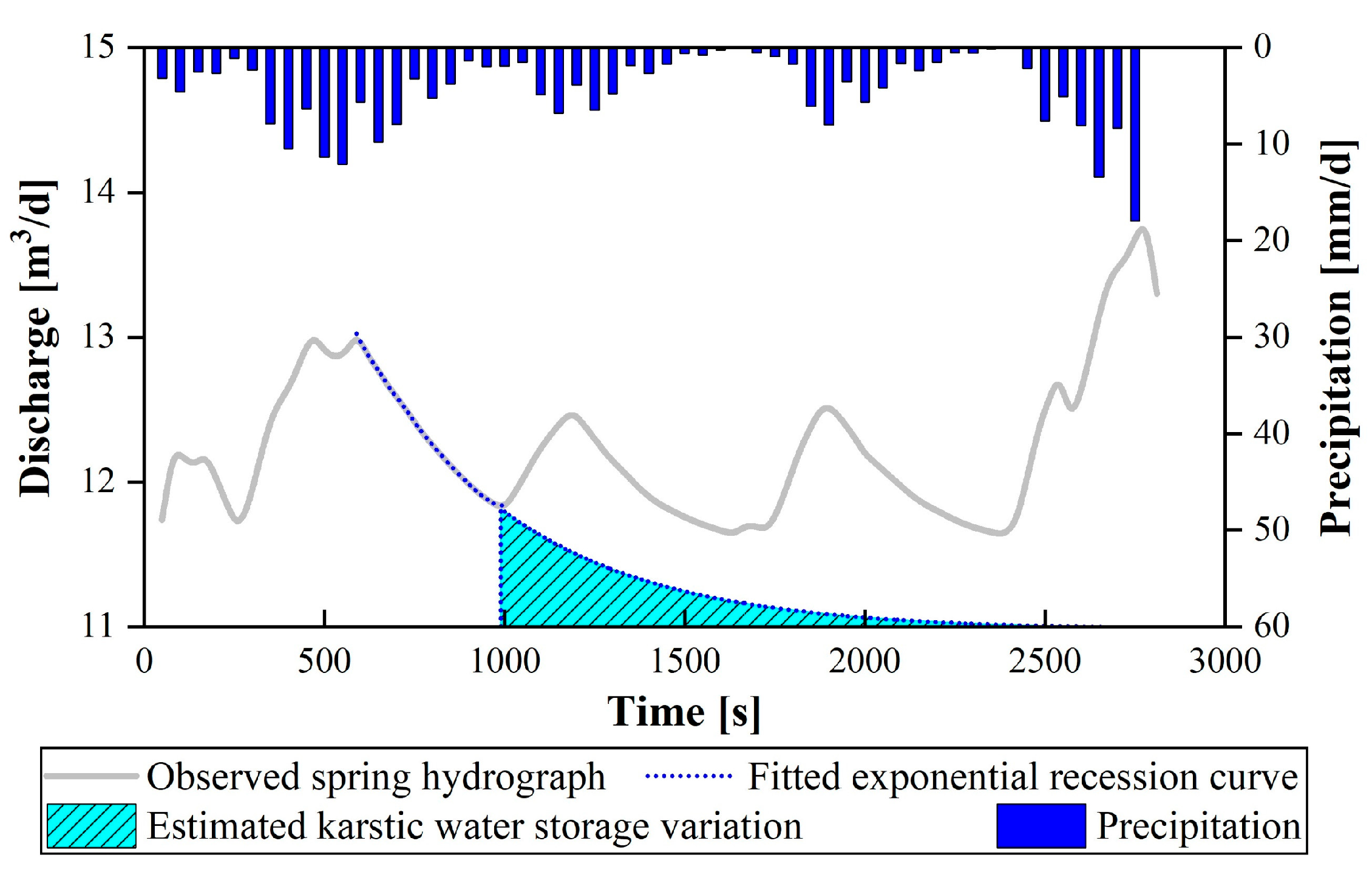
2.2. Analysis Methods

Currently, methods for analyzing karst spring flow curves can be broadly categorized into three main groups, exponential recession methods, non-exponential recession methods, and hybrid recession analysis methods that combine both approaches [27,28]. This study investigates the impact of precipitation on the estimation accuracy of the KWSV via the exponential recession analysis method.

Based on the karst spring flow recession process, Boussinesq [29] and Maillet [30] proposed that spring flow recession curves follow an exponential decay pattern, leading to the development of the exponential recession equation, as shown in Equation (3) which is as follows:

$$Q_t=Q_0{e}^{-\alpha t}$$

(3)

where $Q_t$ denotes the discharge at time t hours after the recession begins; $Q_0$ represents the initial discharge at t = 0; and α represents the recession coefficient.

The KWSV during the spring flow recession could be determined using Equation (4), which is as follows:

$$V_d={\int }_0^t{Q}_0{e}^{-\alpha t}dt$$

(4)

where $V_d$ represents the volume of groundwater discharged during the spring flow recession stage, which corresponds to the KWSV.

According to the Chinese Guidelines for Groundwater Resource Assessment [9], the KWSV refers to the difference between the groundwater storage at the end of the evaluation period and that at the beginning, representing the change in groundwater storage within the karst region during the evaluation period. As shown in Figure 3, at the end of the observed spring flow recession, the remaining karst water storage in the aquifer is more crucial for aquifer management during prolonged droughts than the total storage variation. However, in karst regions, subsequent precipitation events often interrupt the spring recession curve after the last rainfall event, making it challenging to calculate the KWSV from complete observed spring flow recession data following the previous rainfall event. In karst areas where sufficient hydrogeological data are unavailable to establish a high-precision groundwater flow numerical model, researchers can fit an exponential recession curve to the observed spring flow data between the previous and subsequent rainfall events using the Maillet equation. This fitted exponential recession curve is then extrapolated, and the integral of the extrapolated spring recession curve provides an estimate of the KWSV for the extrapolation period, represented by the shaded area in Figure 3. This method is relatively simple and cost effective; however, the estimation accuracy of the KWSV primarily depends on the precision of the extrapolated exponential recession curve.

The calibrated and validated groundwater flow numerical model can accurately simulate the groundwater flow processes observed in physical experiments. Therefore, the simulation results from this numerical model can be regarded as the actual values of KWSV. In contrast, the estimated values of KWSV are obtained by fitting the spring flow recession curve via the Maillet equation and calculating through extrapolation. The estimation accuracy of the KWSV is expressed in terms of the relative error. A larger relative error signifies lower accuracy, whereas a smaller relative error reflects higher accuracy. The formula for calculation is provided in Equation (5), which is as follows:

$$n={\displaystyle \frac{V_a-V_d}{V_a}}\times 100\%$$

(5)

where n represents the relative error of the estimation accuracy of the KWSV; $V_d$ represents the estimated value of the KWSV calculated for the extrapolation period via the Maillet equation; and $V_a$ represents the simulated value of the KWSV calculated from the groundwater flow numerical model for the extrapolation period.

2.3. Numerical Simulation Scheme

For the selection of precipitation events, natural precipitation events are often categorized based on duration and intensity. Considering common types of precipitation in nature, two types of precipitation events are defined: (1) events with the same duration but different intensities and (2) events with the same total volume but different intensities. These two types of events effectively encompass common scenarios in nature, such as light rain, moderate rain, heavy rain, and short-duration intense rainstorms.

For the scenario settings of precipitation events with the same duration but different intensities, the precipitation duration in the initial model was kept constant at 540 s, while the precipitation intensity was set to four different values: 0.010 mm/s, 0.020 mm/s, 0.025 mm/s, and 0.030 mm/s. All other parameters in the initial model remained unchanged. The model was then run, and the spring flow recession curves were recorded. The precipitation event scenario settings are shown in

Table 2. Scenario settings for precipitation events with the same duration but different intensities.

Number	Scenario	Parameter Settings
S01	Basic model	Hydraulic conductivity: layers 2–4; K = 0.015 m/s; μ = 0.06; $\mathrm{conduit}\mathrm{length}:\mathrm{L}=500\mathrm{cm};\mathrm{conduit}\mathrm{roughness}\mathrm{coefficient}=1.0{\mathrm{m}}^{1/3}·{\mathrm{s}}^{-1}$;
S02	Precipitation events with the same duration but different intensities	Intensity: 0.010 mm/s; Duration: 540 s
S03		Intensity: 0.020 mm/s; Duration: 540 s
S04		Intensity: 0.025 mm/s; Duration: 540 s
S05		Intensity: 0.030 mm/s; Duration: 540 s

.

For scenarios with precipitation events of the same total volume but varying intensities, all other parameters in the numerical model were kept constant. In this type of scenario, the total precipitation volume was kept constant at 84 L, while different precipitation durations were set at 100 s, 200 s, 400 s, 600 s, 800 s, and 1000 s. The model was then run, and the spring flow recession data were recorded. The settings for this precipitation event scenario are shown in

Table 3. Scenario settings for precipitation events with the same total volume but different intensities.

Number	Scenario	Parameter Settings
S06	Precipitation events with the same total volume but different intensity	Duration: 100 s; Total volume: 84 L; Intensity: 0.08 mm/s;
S07		Duration: 200 s; Total volume: 84 L; Intensity: 0.04 mm/s;
S08		Duration: 400 s; Total volume: 84 L; Intensity: 0.02 mm/s;
S09		Duration: 600 s; Total volume: 84 L; Intensity: 0.0133 mm/s;
S10		Duration: 800 s; Total volume: 84 L; Intensity: 0.01 mm/s;
S11		Duration: 1000 s; Total volume: 84 L; Intensity: 0.008 mm/s;

.

3. Results and Discussion

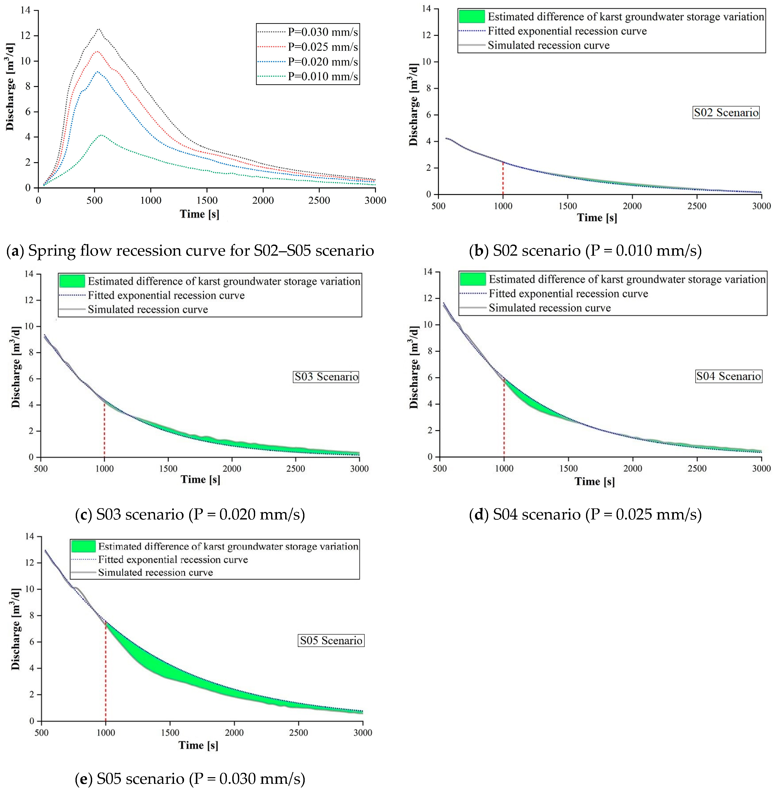
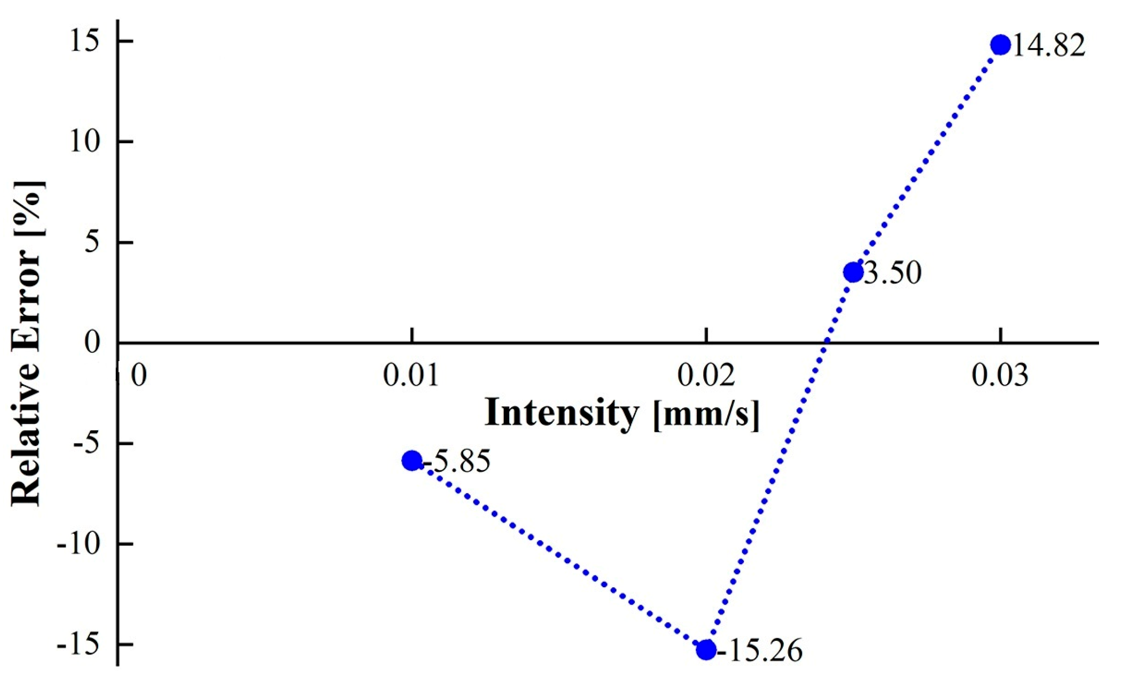
3.1. Precipitation Events with the Same Duration but Different Intensities

Based on the scenarios shown in Table 1, the precipitation intensity was adjusted in the model to simulate precipitation events with the same duration but different intensities. Using numerical modeling outputs, we characterized the spring flow recession dynamics by constructing both simulated recession curves and their corresponding exponential fitting curves (Figure 4). Following the simulation results, we computed the relevant hydrological parameters, including both simulated and estimated values of KWSV, which are systematically tabulated in

Table 4. Calculation of the KWSV under the S02–S05 scenarios.

Scenarios	Exponential Recession Equation	Recession Coefficient	Estimated Value (L)	Simulated Value (L)	Relative Error (%)
S02	y = 8.65e−0.00127x	0.00127	20.53	21.80	−5.85
S03	y = 22.04e−0.00161x	0.00161	30.24	35.69	−15.26
S04	y = 24.76e−0.00142x	0.00142	45.86	44.32	3.50
S05	y = 23.75e−0.00114x	0.00114	68.81	59.93	14.82

Note: “−” indicates that the estimated value of the KWSV is lower than the simulated value.

, and plotted the variation curve of KWSV estimation accuracy, as shown in Figure 5, for comprehensive analysis. These results were then analyzed to explore the impact of precipitation events with the same duration but different intensities on the estimation accuracy of the KWSV.

In this section, the precipitation intensity and duration were implemented in the numerical model according to predefined simulation scenarios. As shown in Figure 4, for scenarios S02–S05, with constant precipitation duration and increasing intensity from 0.010 mm/s to 0.020 mm/s, the estimated values of the KWSV were consistently lower than the simulated values. During this stage, as precipitation intensity increased progressively, the estimation accuracy of KWSV displayed a decreasing trend. However, when precipitation intensity was further elevated to 0.030 mm/s (scenarios S03–S05), the estimated KWSV values gradually converged toward and surpassed the simulated values. Specifically, estimation accuracy initially improved before subsequently declining. A detailed analysis of these scenarios is presented below.

For scenarios S02–S03, where the precipitation duration remains constant but the intensity varies, a higher precipitation intensity results in a greater total precipitation volume, leading to a higher aquifer water level at the end of the precipitation event. The analysis divides the spring flow recession curve into two time periods: 540–1000 s (the initial recession phase) and 1000–3000 s (the later recession phase). In scenario S03, at t = 1000 s, the groundwater level exceeds the elevation of the conduit’s top, placing the conduit flow in a confined state with enhanced drainage capacity. This facilitates rapid discharge of groundwater to the spring outlet as the conduit flows. Conversely, in scenario S02, at t = 1000 s, the groundwater level remains below the elevation of the conduit’s top. During the initial recession phase, the groundwater level gradually decreases, keeping the conduit in an unconfined state with reduced drainage capacity, resulting in a smaller spring flow recession coefficient. Thus, during the initial recession phase (540–1000 s), the spring flow recession coefficient increases with increasing precipitation intensity. The hydrological recession process reveals that, as the spring discharge diminishes progressively, the subsurface water table within the karst aquifer exhibits a descending trend and eventually falls below the elevation of the conduit’s upper boundary. As the conduit’s drainage capacity decreases, groundwater levels decline more slowly, leading to a reduction in the spring flow recession coefficient. Consequently, during the latter stages of recession (1000–3000 s), the simulated spring flow curve is consistently positioned above the exponential decay model derived from the initial phase data (540–1000 s). However, compared with scenario S03, scenario S02 shows that during the initial recession phase (540–1000 s) the groundwater level gradually drops below the conduit’s top elevation, resulting in a smaller difference in the spring flow recession coefficients between the two phases. Consequently, in the latter stages of the recession process (from 1000 to 3000 s), the deviation between the simulated recession curve and the exponential recession curve derived from the initial phase data (spanning 540–1000 s) is moderate, indicating a notable yet limited divergence during this later period. Therefore, for scenarios S02 and S03, an increase in precipitation intensity leads to a gradual decrease in the estimation accuracy of KWSV.

For scenarios S03–S05, as precipitation intensity increases while precipitation duration remains constant the groundwater level rises due to greater storage in the aquifer. In scenarios S04 and S05, the groundwater level exceeds 15 cm, surpassing the top of the second aquifer (karst aquifer), with groundwater fluctuating within the first aquifer (covered loose aquifer). According to the hydrogeological parameters in the numerical model, the covered loose aquifer has a hydraulic conductivity approximately 0.07 times higher than the karst aquifers and a specific yield nearly 1.67 times greater. The recession process reveals distinct effects of aquifer properties on spring flow dynamics. Specifically, the relationship between an aquifer’s specific yield and hydraulic conductivity significantly influences the spring flow recession rate. Aquifers characterized by high specific yield and low hydraulic conductivity exhibit slower declines in groundwater levels and smaller spring flow recession coefficients. In contrast, aquifers with low specific yield and high hydraulic conductivity demonstrate faster declines in groundwater levels and larger spring flow recession coefficients. Considering these factors, in scenarios S04–S05 during the initial recession stage, groundwater fluctuates within the covered loose aquifer. As precipitation intensity increases, this leads to a rise in groundwater levels. Consequently, in scenarios S03–S05 during the initial recession phase, as the groundwater level decreases from the covered loose aquifer to the top of the second aquifer (karst aquifer) the spring flow recession rate remains relatively slow, resulting in smaller recession coefficients. As the spring flow recession continues, there is a corresponding decline in the groundwater level within the aquifer. Compared to the slower decline observed in the covered loose aquifer, the karst aquifer exhibits a more rapid decrease in groundwater levels. This difference accelerates the spring flow recession rate. Therefore, during the 540–1000 s time period, as precipitation intensity increases the overall spring flow recession coefficient gradually decreases.

In the later recession phase (1000–3000 s), at t = 1000 s the groundwater level in scenarios S03–S05 remains above the conduit’s top elevation. As precipitation intensity increases the groundwater level at t = 1000 s increases, keeping the conduit in a confined state with strong drainage capacity. As the spring flow recession progresses, a steady decline in the groundwater level within the aquifer is observed, ultimately resulting in its position dropping below the upper boundary of the conduit. At this transition point, the conduit flow transitions to an unconfined state, resulting in reduced drainage capacity. This change results in a slower rate of spring flow recession and a gradual reduction in the recession coefficient. Furthermore, as precipitation intensity increases, the overall spring flow recession coefficient during the 1000–3000 s period increases. Compared to the recession coefficient during the 540–1000 s period, the difference between the two coefficients becomes more pronounced. In summary, for scenarios S03–S05, as precipitation intensity increases, the simulated spring flow recession curve transitions from surpassing the exponential recession curve derived from the initial phase data (spanning 540–1000 s) to eventually falling below it. This shift causes the simulated karst water storage volume (KWSV) to transition from exceeding the estimated value to falling short of it. Consequently, for scenarios S03–S05, as the precipitation intensity increases the estimation accuracy of the KWSV initially increases and then gradually decreases.

Table 3 shows that as the precipitation intensity increases, the estimation accuracy of KWSV follows the following pattern: it initially decreases, then improves, and subsequently declines again. The relative error between the estimated and simulated values reaches a minimum of 3.5%. This observed behavior is primarily attributed to the significant impact of hydrogeological parameter distributions across different aquifer layers on the spring flow recession rate. As the precipitation volume increases the groundwater level in the aquifer rises, causing fluctuations not only within the karst aquifer but also affecting the covered loose aquifer. These changes slow down the spring flow recession rate during the initial phase of recession. Consequently, the estimation accuracy of the KWSV is closely related to the hydrogeological conditions of the aquifer in which the groundwater level is located. These findings also provide a valuable reference for the calculation of karst water resources.

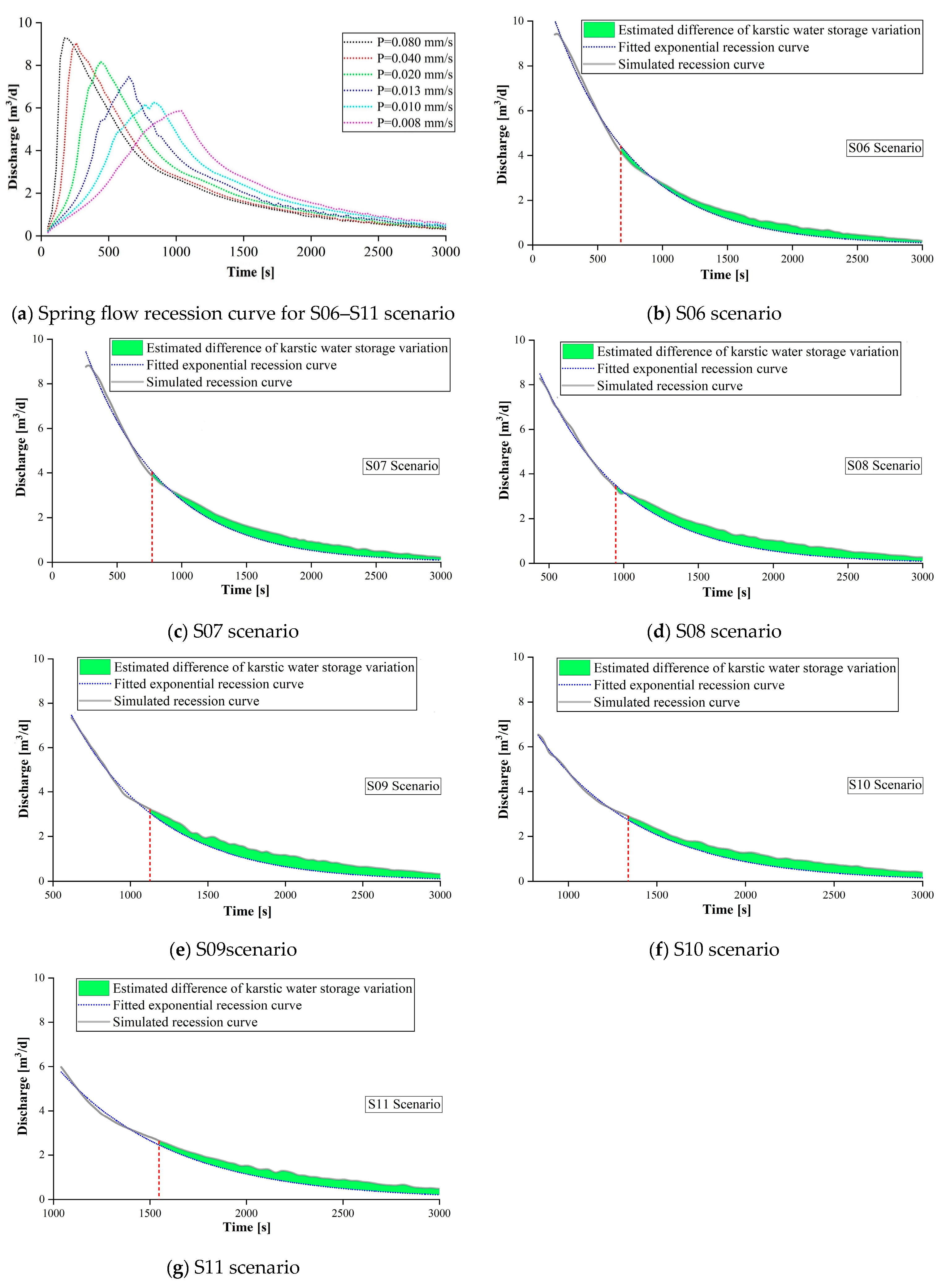
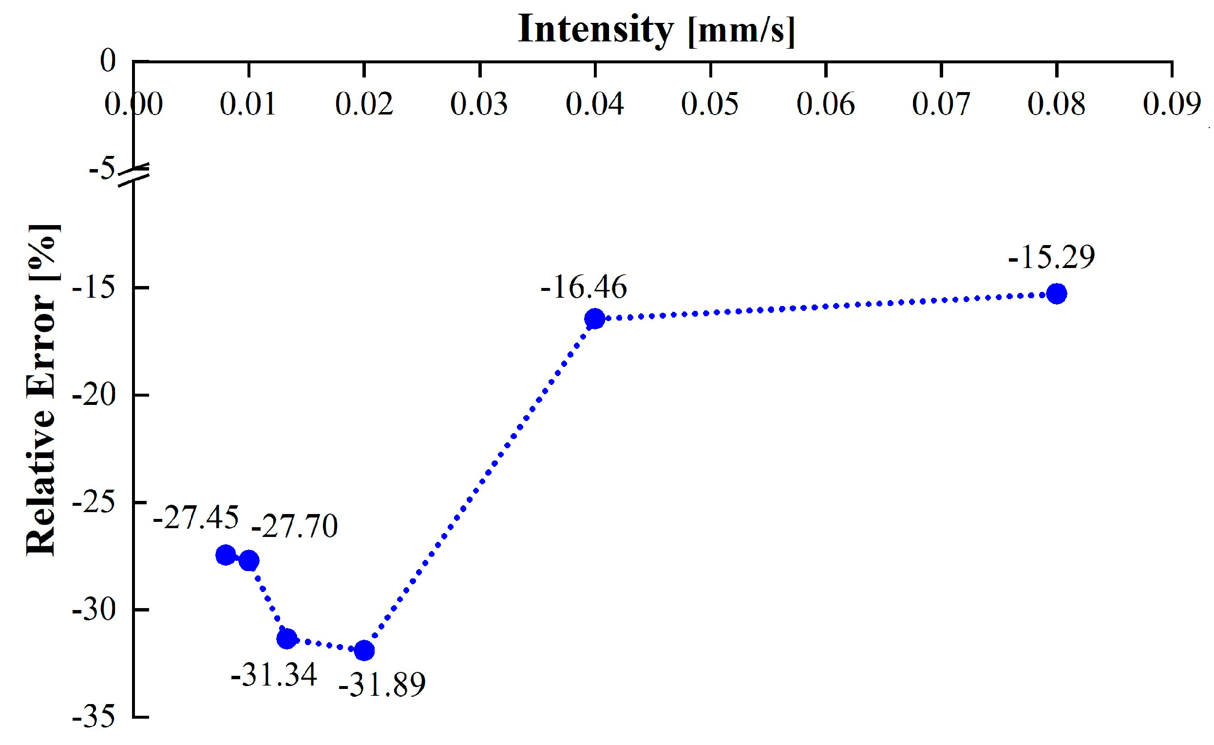
3.2. Precipitation Events with the Same Total Volume but Different Intensities

Using the scenarios from Table 2, the precipitation duration in the model was adjusted to simulate precipitation events with the same total volume but varying intensities. Using the numerical model results, both the simulated spring flow recession curves and the fitted exponential recession curves for the recession phase were generated. In this section, the fitted exponential recession curves were derived from the spring flow data within 540 s after the initial recession time, as shown in Figure 6. Moreover, the simulated and estimated KWSV values during the spring flow recession were determined, as presented in

Table 5. Calculation of the karstic water storage variation under the S06–S11 scenarios.

Scenarios		Exponential Recession Equation	Recession Coefficient	Estimated Value (L)	Simulated Value (L)	Relative Error (%)
S06	t = 100 s, P = 0.08 mm/s	y = 13.21e−0.00161x	0.00161	31.03	36.63	−15.29
S07	t = 200 s, P = 0.04 mm/s	y = 14.46e−0.00165x	0.00165	27.80	33.28	−16.46
S08	t = 400 s, P = 0.02 mm/s	y = 18.99e−0.00180x	0.00180	20.25	29.74	−31.89
S09	t = 600 s, P = 0.0133 mm/s	y = 22.25e−0.00177x	0.00177	19.11	27.84	−31.34
S10	t = 800 s, P = 0.010 mm/s	y = 26.86e−0.00171x	0.00171	17.34	23.98	−27.70
S11	t = 1000 s, P = 0.008 mm/s	y = 33.05e−0.00168x	0.00168	15.35	21.16	−27.45

Note: “−” indicates that the estimated value of the KWSV is lower than the simulated value.

, and the variation curve of KWSV estimation accuracy was plotted, as shown in Figure 7. A comparative analysis was conducted to explore the influence of precipitation events with the same total volume but different intensities on the estimation accuracy of the KWSV.

This section presents the precipitation intensity and duration for each simulation scenario. With a fixed total precipitation volume, the precipitation duration directly influences the intensity: a shorter duration corresponds to a higher intensity whilst a longer duration results in a lower intensity. As shown in Figure 7, scenarios S06–S11 demonstrate that for the same total precipitation volume, as the precipitation duration increases from 100 s to 1000 s the estimated values of the KWSV consistently remain below the simulated values. Furthermore, the estimation accuracy of the KWSV initially decreases but then increases with increasing precipitation duration. A detailed analysis of each scenario is provided below.

For scenarios S06–S08, as shown in Table 4, under the condition of constant total precipitation volume, the estimation accuracy of KWSV gradually decreases as precipitation duration increases. The analysis of the spring flow recession phase is divided into two stages: the first stage is within 540 s after the recession start time and the second stage is from 540 s after the recession start time to 3000 s. A detailed analysis of these stages is provided below.

For the initial stage of the recession process (the first 540 s after the recession starts) under the condition of constant total precipitation volume, as the precipitation duration increases the precipitation intensity gradually decreases. In scenarios S06–S07, the groundwater level rises above the top of the second aquifer (karst aquifer) and fluctuates within the first aquifer (covered loose aquifer). Conversely, in scenario S08 the groundwater level fluctuates within the second aquifer (the karst aquifer). Based on the hydrogeological parameters from the numerical model, the covered loose aquifer exhibits lower hydraulic conductivity and higher specific yield compared to the karst aquifer. This results in greater water release per unit drop in groundwater level but a slower groundwater movement velocity. In scenarios S06–S07, the initial groundwater level at recession onset is within the covered loose aquifer; the higher the groundwater level in this aquifer is at the start of recession the greater its influence on the recession coefficient during the initial stage, resulting in a lower recession coefficient. Therefore, in scenarios S06–S08, as the precipitation duration increases and the precipitation intensity decreases, the initial groundwater level transitions from the covered loose aquifer to the karst aquifer. This shift causes the initial-stage recession coefficient to gradually increase.

During the stage from 540 s after the recession started to 3000 s, as the recession progresses the groundwater level in the aquifer gradually decreases. At 540 s after the recession started, the groundwater levels in scenarios S06–S08 decreased sequentially. Among these, in scenario S06 the groundwater level in the aquifer is the highest at approximately 8.0 cm, whereas in scenario S08 it is the lowest at approximately 6.6 cm. As the spring flow recession continues, in scenario S08 the groundwater level drops below the elevation of the conduit roof first, causing the conduit flow to transit to an unconfined state. This reduction in drainage capacity slows the spring flow recession rate. Therefore, in scenarios S06–S08 the fitting degree between the simulated spring flow recession curve and the spring flow exponential recession curve fitted with the initial stage recession data becomes progressively worse, that is, the accuracy of KWSV estimation decreases as the precipitation duration increases. This gradual reduction in estimation accuracy reflects how variations in groundwater dynamics across different recession stages impact model performance.

For scenarios S09–S11, as the precipitation duration increases the groundwater level in the aquifer gradually drops after the precipitation event concludes. In scenarios S09–S11, the groundwater levels fluctuate within the second and third aquifers (karst aquifers) at the start of the recession and gradually decrease. Compared with scenario S09, in scenarios S10–S11 the groundwater levels in most areas of the aquifer fall below the roof of the conduit, thereby causing the conduit flow to transition to an unconfined state. This reduction in drainage capacity slows the spring flow recession rate, resulting in a decreased recession coefficient. Consequently, in scenarios S09 to S11 the recession coefficients during the initial recession stage generally decreased progressively.

For the period from 540 s after the onset of recession to 3000 s, as the recession continues the groundwater levels in scenarios S10–S11 fall below the top of the conduit and continue to decrease. As a result, the conduit’s drainage capacity continues to decrease, leading to a sustained decline in the spring flow recession rate. The difference in recession rates between the initial and subsequent stages also becomes smaller. As a result, in scenarios S09–S11 the alignment between the simulated spring flow recession curve and the exponential recession curve (fitted with the initial recession data) progressively improved, indicating that the KWSV estimation accuracy increased with the precipitation duration before stabilizing.

As shown in Table 4, under a constant total precipitation volume the estimation accuracy of the KWSV initially decreases, then increases, and eventually stabilizes as the precipitation duration increases. The minimum relative error between the estimated and simulated values is 15.29%. Under the same total precipitation volume, different precipitation durations result in varying groundwater levels in the aquifer at the start of the spring flow recession phase—shorter precipitation durations correspond to higher groundwater levels. The hydrogeological properties of the aquifer containing the groundwater level during the initial recession phase play a crucial role in determining the spring flow recession rate. As such, the effect of precipitation events on KWSV estimation accuracy is mainly influenced by the characteristics of the aquifer where the groundwater level stabilizes after the event.

3.3. Limitations

The errors discussed in this study mainly stem from uncertainties in the simulation of precipitation events and the estimation of karst water storage variation. However, there are additional sources of uncertainty when simulating karst systems, including the hydraulic conductivity and specific yield of the matrix or fractures, the structure of the conduits, and the setting of boundary conditions. These uncertainties may have a more complex impact on the estimation accuracy of the KWSV. Compared to other uncertainties, this study focuses on analyzing the influence of precipitation processes on estimation error of KWSV within a known range of hydrogeological conditions and parameters. In practical applications, estimation errors of KWSV under different precipitation events may affect the rational development and management of karst water resources, particularly in water resource allocation, drought warning, and source water protection. Due to the high heterogeneity of karst aquifer systems, inaccurate estimations may lead to misjudgments about groundwater recharge processes, thereby affecting the scientific validity and effectiveness of water resource management decisions. Therefore, understanding and evaluating the estimation accuracy of KWSV is crucial for improving the reliability of model predictions and their applicability in practice.

In the physical experiment model and the corresponding equivalent porous medium–conduit coupled groundwater flow numerical model established in this study, the karst matrix parameters exhibit relatively simple distributions, and the conduit structure is also straightforward. Additionally, the unsaturated zone was not considered. However, it is important to recognize that real-world karst aquifer systems are typically highly heterogeneous and strongly nonlinear hydrological systems. The existence of covered surface karst zones and multi-layer conduit systems may have more complex effects on the process of spring flow recession. Therefore, in future research, the heterogeneity of karst hydrogeological parameters should be incorporated into the model, including considering the unsaturated zone and conduit structure types. These aspects will be further explored as future research directions.

4. Conclusions

Based on the hydrogeological conditions of a typical covered karst aquifer system in northern China, this study developed a three-dimensional physical experiment model and a corresponding equivalent porous medium–conduit coupled groundwater flow numerical model. By simulating various rainfall patterns, we analyzed how these events influence the estimation accuracy of karst water storage volume (KWSV).

(1) Under conditions of the same precipitation duration, the estimation accuracy of the KWSV follows a “decrease–increase–decrease” trend with increasing precipitation intensity. When the precipitation intensity is low, the groundwater levels fluctuate within the karst aquifer. Once the water level drops below the top of the karst conduit the decline rate in the water level becomes slower, leading to a reduced spring flow recession rate and causing the simulated values to exceed the estimated values. Conversely, at higher rainfall intensities, the groundwater level rises rapidly into the covered loose sediment layer. Due to the varying hydrogeological characteristics across different aquifers, the alignment between the spring flow recession curve and the fitted curve changes significantly, causing the simulated values to transition from being greater than the estimated values to being lower than them.

(2) Under the condition of the same total precipitation volume, as the precipitation duration increases the estimation accuracy of KWSV tends to gradually decrease–increase–stabilize. Precipitation events with short durations but high intensities cause the groundwater level to rise rapidly into the covered loose aquifer. Due to its low hydraulic conductivity and high specific yield characteristics, the decline in groundwater level becomes slower, resulting in a lower spring flow recession coefficient and larger estimation errors. As the precipitation duration extends, the groundwater level gradually stabilizes within the karst aquifer, resulting in a better alignment between the simulated spring flow recession curve and the exponential fitting curve. Consequently, this results in more stable estimation accuracy for KWSV.

This study indicates that different precipitation events significantly affect the estimation accuracy of the KWSV, and the primary mechanism underlying this relationship is closely tied to the hydrogeological parameter characteristics of the aquifer where the groundwater level resides during the recession stage. Notably, in composite aquifer systems, critical parameters such as hydraulic conductivity and specific yield play a decisive role in shaping the dynamic characteristics of the spring flow recession process. The research findings not only enhance our understanding of hydrological processes within karst aquifer systems but also provide crucial references for the rational development and sustainable management of karst water resources under varying precipitation scenarios.

References

1. Bakalowicz, M. Karst groundwater: A challenge for new resources. Hydrogeol. J. 2005, 13, 148–160. [Google Scholar]
2. Koit, O.; Mayaud, C.; Kogovšek, B.; Vainu, M.; Terasmaa, J.; Marandi, A. Surface water and groundwater hydraulics of lowland karst aquifers of Estonia. J. Hydrol. 2022, 610, 127908. [Google Scholar]
3. Goldscheider, N.; Chen, Z.; Auler, A.; Bakalowicz, M.; Broda, S.; Drew, D.; Hartmann, J.; Jiang, G.; Moosdorf, N.; Stevanovic, Z.; et al. Global distribution of carbonate rocks and karst water resources. Hydrogeol. J. 2020, 28, 1661–1677. [Google Scholar] [CrossRef]
4. Dagès, C.; Voltz, M.; Bsaibes, A.; Prévot, L.; Huttel, O.; Louchart, X.; Garnier, F.; Negro, S. Estimating the role of a ditch network in groundwater recharge in a Mediterranean catchment using a water balance approach. J. Hydrol. 2009, 375, 498–512. [Google Scholar]
5. Weatherl, R.K.; Salgado, M.J.H.; Ramgraber, M.; Moeck, C.; Schirmer, M. Estimating surface runoff and groundwater recharge in an urban catchment using a water balance approach. Hydrogeol. J. 2021, 29, 2411–2428. [Google Scholar]
6. Yi, Y.; Brock, B.E.; Falcone, M.D.; Wolfe, B.B.; Edwards, T.W. A coupled isotope tracer method to characterize input water to lakes. J. Hydrol. 2008, 350, 1–13. [Google Scholar]
7. Borghi, A.; Renard, P.; Cornaton, F. Can one identify karst conduit networks geometry and properties from hydraulic and tracer test data? Adv. Water Resour. 2016, 90, 99–115. [Google Scholar]
8. Chen, X.; Zhang, Y.; Zhou, Y.; Zhang, Z. Analysis of hydrogeological parameters and numerical modeling groundwater in a karst watershed, southwest China. Carbonates Evaporites 2013, 28, 89–94. [Google Scholar] [CrossRef]
9. Dafny, E.; Burg, A.; Gvirtzman, H. Effects of Karst and geological structure on groundwater flow: The case of Yarqon-Taninim Aquifer, Israel. J. Hydrol. 2010, 389, 260–275. [Google Scholar]
10. Basha, H.A. Flow recession equations for karst systems. Water Resour. Res. 2020, 56, e2020WR027384. [Google Scholar]
11. Fiorillo, F. The recession of spring hydrographs, focused on karst aquifers. Water Resour. Manag. 2014, 28, 1781–1805. [Google Scholar]
12. Felton, G.K.; Currens, J.C. Peak flow rate and recession-curve characteristics of a karst spring in the Inner Bluegrass, central Kentucky. J. Hydrol. 1994, 162, 99–118. [Google Scholar]
13. Ding, H.; Zhang, X.; Chu, X.; Wu, Q. Simulation of groundwater dynamic response to hydrological factors in karst aquifer system. J. Hydrol. 2020, 587, 124995. [Google Scholar]
14. Martin, J.M.; Screaton, E.J.; Martin, J.B. Monitoring well response to karst conduit head fluctuations: Implications for fluid exchange and matrix transmissivity in the Floridan aquifer. Geol. Soc. America Spec. 2006, 404, 209–217. [Google Scholar]
15. Guo, X.; Huang, K.; Li, J.; Kuang, Y.; Chen, Y.; Jiang, C.; Luo, M.; Zhou, H. Rainfall–Runoff Process Simulation in the Karst Spring Basins Using a SAC–Tank Model. J. Hydrol. Eng. 2023, 28, 04023024. [Google Scholar]
16. Kovács, A.; Perrochet, P.; Király, L.; Jeannin, P.-Y. A quantitative method for the characterisation of karst aquifers based on spring hydrograph analysis. J. Hydrol. 2005, 303, 152–164. [Google Scholar]
17. Zimmerman, R.W.; Bodvarsson, G.S. Hydraulic conductivity of rock fractures. Transp. Porous Media 1996, 23, 1–30. [Google Scholar]
18. Neuman, S.P. On methods of determining specific yield. Groundwater 1987, 25, 679–684. [Google Scholar]
19. Abirifard, M.; Birk, S.; Raeisi, E.; Sauter, M. Dynamic volume in karst aquifers: Parameters affecting the accuracy of estimates from recession analysis. J. Hydrol. 2022, 612, 128286. [Google Scholar]
20. Shu, L.; Zou, Z.; Li, F.; Wu, P.; Chen, H.; Xu, Z. Laboratory and numerical simulations of spatio-temporal variability of water exchange between the fissures and conduits in a karstic aquifer. J. Hydrol. 2020, 590, 125219. [Google Scholar]
21. Chang, Y.; Wu, J.; Liu, L. Effects of the conduit network on the spring hydrograph of the karst aquifer. J. Hydrol. 2015, 527, 517–530. [Google Scholar]
22. Peterson, E.W.; Wicks, C.M. Assessing the importance of conduit geometry and physical parameters in karst systems using the storm water management model (SWMM). J. Hydrol. 2006, 329, 294–305. [Google Scholar]
23. Huang, F.; Gao, Y.; Hu, X.; Wang, X.; Pu, S. Interaction mechanism between the karst aquifer and stream under precipitation infiltration recharge. EGUsphere 2025, 2025, 1–56. [Google Scholar]
24. Mohammadi, Z.; Shoja, A. Effect of annual rainfall amount on characteristics of karst spring hydrograph. Carbonates Evaporites 2014, 29, 279–289. [Google Scholar]
25. Chang, W.; Wan, J.; Tan, J.; Wang, Z.; Jiang, C.; Huang, K. Responses of spring discharge to different rainfall events for single-conduit karst aquifers in Western Hunan province, China. Int. J. Environ. Res. Pub. Health 2021, 18, 5775. [Google Scholar]
26. Li, Y.; Shu, L.; Wu, P.; Zou, Z.; Zhou, T.; Huang, L. Rainfall events-spring flow relationship and karst flow component analysis in a conduit-matrix coupled system. Hydrol. Process 2023, 37, e14990. [Google Scholar]
27. Solórzano-Rivas, S.C.; Werner, A.D.; Robinson, N.I. Assessing the reliability of exponential recession in the water table fluctuation method. Adv. Water Resour. 2024, 193, 104821. [Google Scholar]
28. Li, G.; Goldscheider, N.; Field, M.S. Modeling karst spring hydrograph recession based on head drop at sinkholes. J. Hydrol. 2016, 542, 820–827. [Google Scholar]
29. Boussinesq, J. Sur un mode simple d’écoulement des nappes d’eau d’infiltration à lit horizontal, avec rebord vertical tout autour lorsqu’une partie de ce rebord est enlevée depuis la surface jusqu’au fond. CR Acad. Sci. 1903, 137, 11–23. [Google Scholar]
30. Maillet, E.T. Essais D’hydraulique Souterraine & Fluviale; A. Hermann: Paris, France, 1905. [Google Scholar]
Figure 1. Schematic diagram of the physical experimental model.
Water 17 00986 g001
Figure 2. Three-dimensional diagram of the groundwater flow numerical model.
Water 17 00986 g002
Figure 3. Schematic of the estimated KWSV.
Water 17 00986 g003
Figure 4. Simulated and fitted recession curves under the scenario of precipitation events with the same duration but different intensities.
Water 17 00986 g004
Figure 5. The estimation accuracy of the KWSV under the precipitation events with the same duration but different intensities.
Water 17 00986 g005
Figure 6. Simulated and fitted recession curves under the scenario of precipitation events with the same total volume but different intensities.
Water 17 00986 g006
Figure 7. The estimation accuracy of the KWSV under precipitation events with the same total volume but different intensities.
Water 17 00986 g007