Selection of a Turbulence Model for Wave Evolution on a New Ecological Hollow Cube

Abstract

A suitable turbulence model is needed for numerical simulations to accurately simulate the wave evolution and hydrodynamic performance of the new ecological hollow cube. The new ecological hollow cube is an improvement upon traditional designs, as it can grow plants to dissipate wave energy. In this study, the open-source computational fluid dynamics (CFD) software OpenFOAM v2206 is used as the computational platform to analyze and evaluate the numerical results of four turbulence models, i.e., the standard k-ε, steady k-ω shear stress transfer (SST), buoyancy-corrected k-ω SST, and large eddy simulation (LES) models, by using three mesh systems (with grid counts of 0.89, 2.92, and 8.91 million grids, respectively). Comparison of the numerical results from the four turbulence models reveals that the stabilized k-ω SST turbulence model provides better results for simulating the complex wave evolution process on the cube and effectively captures the wave free surface. In contrast, the other models exhibit a greater grid dependency. The stabilized k-ω SST model more accurately captures the wave run-up and reflection coefficient better than other turbulence models do. Therefore, the stabilized k-ω SST model is selected as the most suitable turbulence model for hydrodynamic modeling of the new ecological hollow cube.

1. Introduction

Offshore infrastructure in coastal cities is facing increasing threats from both rapid urbanization and a rise in severe weather events, including the destructive forces of typhoons and storm surges. It is a major engineering challenge to protect coastal structures from being eroded by waves [1]. In coastal engineering, armor blocks are frequently utilized as a form of protective armor unit. Dams, embankments, seawalls, and breakwaters are frequently shielded from wave erosion through the use of armor blocks. In particular, based on the traditional hollow cube, the improved new ecological hollow cube has been proven to have excellent wave dissipation [2]. It is important to protect critical coastal infrastructure from wave erosion and impact.

Due to the complexities of wave behavior, physical model tests and numerical simulations are standard techniques for analyzing how waves evolve around armor blocks and how effectively these blocks perform under wave action [3]. However, performing physical model tests for armor blocks in wave flumes is expensive, and it takes time to fabricate the blocks. Numerical simulation is important in researching armor blocks as an effective and complementary tool. The complex hydrodynamics associated with wave interaction over novel ecological hollow cube structures necessitates a comprehensive evaluation of the resulting wave turbulence. To guarantee the reliability of numerical simulations that depict wave interaction with innovative ecological hollow cubes, it is crucial to utilize an appropriate model for turbulence during the calculation process.

Two major categories of turbulence models, RANS and LES, have undergone substantial development in recent decades. Within the RANS category, several specific model types exist, including those based on zero-equation, one-equation, two-equation, and Reynolds stress approaches. However, this model is seldom used in practical engineering because turbulent pulsation is neglected, and the mixing length can be easily obtained only for simple flows. The Spalart–Allmaras model [4] is a notable instance of a one-equation turbulence model, prized for its utility in simulating flow phenomena in aerospace and mechanical engineering applications. Due to their versatility and relative simplicity, two-equation turbulence models, with the k-ε and k-ω models being prominent examples, are not only applied extensively across diverse disciplines, but also continue to be the focus of ongoing research and enhancement efforts. In practical applications, the standard k-ε model [5], the RNG k-ε model [6], the standard k-ω model [7], and the k-ω SST model [8] are frequently selected as examples of two-equation turbulence models, in addition to several other available alternatives. The classical Reynolds stress models include the k-ε model [9] and the Wilcox k-ω model [10]. However, the Reynolds stress model is computationally intensive and difficult to converge, so it is not widely used. In the LES turbulence model, the larger, more energetic turbulent eddies are directly computed using a subgrid-scale approach, while the effects of smaller, subgrid-scale eddies are represented through appropriate turbulence models. Within the realm of LES turbulence modeling techniques, the Smagorinsky model [11] is a particularly celebrated and frequently employed approach. The LES approach to turbulence modeling often proves impractical for many engineering applications due to its intense computational requirements and difficulties in resolving flow near solid walls. In contrast, RANS models offer a computationally affordable and versatile alternative, making them a popular choice for a broad spectrum of engineering problems. While the RANS model offers advantages in terms of computational efficiency, it also exhibits recognized shortcomings in wave hydrodynamics simulations. Notably, many researchers have documented a tendency for this model to predict excessive wave decay and over-predict the levels of turbulent kinetic energy, resulting in results that deviate substantially from experimental measurements [12]. Seeking to remedy the aforementioned issues, Ref. [13] introduced a particular modification to the standard k-ω model. Recognizing the tendency for the k-ω shear stress transfer (SST) model to generate artificially high levels of turbulent kinetic energy in regions near free surfaces, Ref. [14] proposed an improvement in the form of a buoyancy correction term [15] designed to mitigate this issue. Recognizing that the k-ω SST model tended to overestimate turbulent kinetic energy, Ref. [16] proposed a refinement to the model by correcting the formulation of its vortex viscosity, a change that effectively suppressed the excessive generation of turbulence.

Obtaining trustworthy and meaningful insights from computational fluid dynamics (CFD) simulations hinges on the careful selection and implementation of a turbulence model that is appropriate for the specific physical phenomena under investigation. Aiming to elucidate the hydrodynamic behavior of a sloped surf zone, Ref. [17] conducted a series of simulations using various RANS turbulence models, and the accuracy of these simulations was assessed by comparing the predicted results with experimental data obtained by [18]. Based on their analysis, the standard k-ε model demonstrated a greater capacity to accurately simulate turbulent phenomena within the surf zone compared to the performance of the RNG k-ε model. In their investigation, Ref. [19] compared numerical simulations with experimental data obtained from a wave flume and found that the k-ω SST model more accurately represented the free surface compared to the k-ε model. Ref. [20] conducted a study to characterize the forces, velocities, and other hydrodynamic properties of waves as they propagate past a cylindrical structure, utilizing a selection of turbulence models to simulate the flow. The hydrodynamic characteristics of the buoyancy-modified k-ω SST model and the stabilized k-ω SST model effectively reduce the turbulent kinetic energy of the waves before they pass through the cylinder. However, the obtained wave impact force is smaller than that in the experimental data. Ref. [21] studied the wave evolution and hydrodynamic characteristics of a coral reef berm breakwater. A comprehensive comparison of the numerical output generated by three distinct turbulence models indicated that the stabilized k-ω SST model exhibited a superior capability in producing consistent and accurate simulations of the complex wave propagation and breaking processes that occur on a reef beach.

Prior investigations have employed initial physical model testing and numerical simulations to explore the hydrodynamic characteristics of armor blocks and to gain a better understanding of the intricate processes involved in the evolution of complex waves. Typical approaches in the study of armour blocks, typical methods include physical modeling tests [22] and numerical simulations [23]. In the existing literature, numerical simulations have often been limited to the application of a single turbulence model, such as the standard k-ε, the standard k-ω, or the stabilized k-ω SST formulation. Furthermore, these studies have not typically addressed the important issue of grid sensitivity, meaning they have not evaluated whether the results are influenced by the size and spacing of the computational cells used in the simulation. To the authors’ knowledge, there is no relevant work on the comparative hydrodynamic characteristics of a new ecological hollow cube using different turbulence models, which is used as the research condition in this study, and its hydrodynamic characteristics are comparatively investigated by four different turbulence models.

This paper is organized as follows: Section 2 presents the numerical model setup. Section 3 describes the new ecological hollow cube, numerical model meshing, and data postprocessing of wave run-up and the reflection coefficient. Section 4 evaluates the effects of grid and turbulence modeling on various parameters of the hydrodynamic model, such as the relative wave run-up and reflection coefficient. Section 5 presents the summary and conclusions of this research.

2. Numerical Model

2.1. Governing Equations

The olaFlow, a two-phase solver, conducted the numerical model of the new ecological hollow cube. Ref. [24] developed the computational module IHFOAM as a platform, which was later developed into olaFlow [24]. As one of the extended solvers for OpenFOAM v2206, olaFlow uses the finite volume method (FVM) for the numerical discretization of the Reynolds-averaged Navier–Stokes (RANS) equations and relies on the volume of fluid (VOF) approach to accurately represent the interface between two distinct fluid phases. It can effectively handle structures with complex shapes and various wave interactions. Furthermore, it incorporates sophisticated wave generation and active absorption boundary algorithms [25], contributing to both a decrease in computational expense and an increase in the precision of the simulations. Considering the complexity of the new ecological hollow cube, olaFlow is chosen as the computational platform in this study. In order to reduce the computational cost of the simulations, a variable time-stepping scheme was employed. Furthermore, to maintain numerical stability and accuracy, the Courant number, a measure of numerical diffusion, was kept below a value of 0.25.

2.2. Turbulence Models

To determine the applicability of different turbulence models in simulating the hydrodynamic characteristics of new ecological hollow cubes, the standard k-ε model, the stabilized k-ω SST model, the buoyancy-modified k-ω SST model, and the LES model were initially used in this study. Ref. [2] conducted a series of physical modeling experiments for new ecological hollow cubes, and Ref. [26] conducted numerical simulations adopting the RNG k-ε turbulent model. Despite the satisfactory agreement between numerical and experimental results, the RNG k-ε turbulence model was not employed in this investigation due to its slow convergence and prohibitive computational expense in large-scale simulations. Ultimately, this study utilizes only four turbulent models: the standard k-ε model, the stabilized k-ω SST model, the buoyancy-modified k-ω SST model, and the LES model.

2.2.1. Standard k-ε Model

The standard k-ε turbulence model assumes that the flow is fully turbulent and that the eddy viscosities are isotropic, so the model applies to a flow field that fully develops into a turbulent state. The two equations for k and ε are as follows:

$${\displaystyle \frac{\partial \left(\rho k\right)}{\partial t}}+{\displaystyle \frac{\partial \left(\rho {ku}_i\right)}{\partial x_i}}={\displaystyle \frac{\partial }{\partial x_j}}\left[{\displaystyle \frac{{\mu }_t}{{\sigma }_k}}{\displaystyle \frac{\partial k}{\partial x_j}}\right]+2{\mu }_t{S_{ij}S}_{ij}-\rho \epsilon$$

(1)

$${\displaystyle \frac{\partial \left(\rho \epsilon \right)}{\partial t}}+{\displaystyle \frac{\partial \left(\rho {\epsilon u}_i\right)}{\partial x_i}}={\displaystyle \frac{\partial }{\partial x_j}}\left[{\displaystyle \frac{{\mu }_t}{{\sigma }_{\epsilon }}}{\displaystyle \frac{\partial \epsilon }{\partial x_j}}\right]+{\mathrm{C}}_{1\epsilon }{\displaystyle \frac{\epsilon }{k}}2{\mu }_t{S_{ij}S}_{ij}-{\mathrm{C}}_{2\epsilon }{\displaystyle \frac{{\epsilon }^2}{k}}$$

(2)

where $S_{ij}$ is the tensor of the average strain rate, $S_{ij}$ = ${\displaystyle \frac{1}{2}}\left({\displaystyle \frac{\partial u_i}{\partial x_j}}+{\displaystyle \frac{\partial u_j}{\partial x_i}}\right)$, and the dynamic eddy viscosity ${\mu }_t$ is determined by the following:

$${\mu }_t=\rho {\mathrm{C}}_{\mu }{\displaystyle \frac{k^2}{\epsilon }}$$

(3)

The constants $C_{1\epsilon }$, $C_{2\epsilon }$, $C_{\mu }$, ${\partial }_k$, and ${\partial }_{\epsilon }$ involved in this turbulent model were calibrated by fitting a large amount of turbulence test data, as listed in

Table 1. Reference values of the coefficients in the k-ε turbulence model.

Coefficient	${\mathit{C}}_{\mathit{\mu }}$	${\mathit{\sigma }}_{\mathit{K}}$	${\mathit{\sigma }}_{\mathit{ϵ}}$	${\mathit{C}}_{1\mathit{ϵ}}$	${\mathit{C}}_{2\mathit{ϵ}}$
Value	0.09	1	1.30	1.44	1.92

.

2.2.2. Stabilized k-ω SST Model

To mitigate the excessive increase in turbulent energy and eddy viscosity within the fluid domain, [16] explored the implementation of both buoyancy and eddy viscosity corrections within the framework of the k-ω SST model [8]. The subsequent equations of the stabilized k-ω SST model are presented below:

$${\displaystyle \frac{\partial \left(\rho k\right)}{\partial t}}+{\displaystyle \frac{\partial \left(\rho {ku}_i\right)}{\partial x_i}}={\displaystyle \frac{\partial }{\partial x_j}}\left[(\mu +{{\sigma }_K\mu }_t){\displaystyle \frac{\partial k}{\partial x_j}}\right]+P_k+G_b-{\beta }^{\ast }\rho \omega k$$

(4)

$${\displaystyle \frac{\partial \left(\rho \omega \right)}{\partial t}}+{\displaystyle \frac{\partial \left(\rho {\omega u}_i\right)}{\partial x_i}}={\displaystyle \frac{\partial }{\partial x_i}}\left[(\mu +{{\sigma }_{\omega }\mu }_t){\displaystyle \frac{\partial \omega }{\partial x_i}}\right]+\alpha \rho S^2-\beta \rho {\omega }^2+2(1-F_1){\displaystyle \frac{\rho {\sigma }_{\omega 2}}{\omega }}{\displaystyle \frac{\partial k}{\partial x_i}}{\displaystyle \frac{\partial \omega }{\partial x_i}}$$

(5)

Within this particular turbulence model, the correction factor α_βs, used in the buoyancy term G_b, is assigned a value of 1.36. Subsequently, the calculation of turbulent viscosity proceeds as follows:

$$v_t=a_{1}k/max(a_1\omega ,F_2\sqrt{P_0},a_1{\lambda }_2{\displaystyle \frac{\beta }{{\beta }^{\ast }a}}{\displaystyle \frac{P_0}{P_{\Omega }}}\omega )$$

(6)

where the stress limitation factor ${\lambda }_2$ is 0.05, $P_0$ = 2$S_{ij}{S}_{ij}$,$P_{\Omega }$ = 2${\Omega }_{ij}{\Omega }_{ij}$, and the average rotation rate tensor ${\Omega }_{ij}$ = $\left(\partial u_i/\partial x_j-\partial u_j/\partial x_i\right)/2$.

2.2.3. Buoyancy-Modified k-ω SST Model

Building upon the foundation of the k-ω SST model [8,14] engineered a variant that accounts for buoyancy, resulting in a buoyancy-modified k-ω SST model, which avoids excessive turbulent kinetic energy at the gas–liquid interface by introducing a buoyancy correction term. The k and ω equations are as follows:

$${\displaystyle \frac{\partial \left(\rho k\right)}{\partial t}}+{\displaystyle \frac{\partial \left(\rho {ku}_i\right)}{\partial x_i}}={\displaystyle \frac{\partial }{\partial x_j}}\left[(\mu +{{\sigma }_K\mu }_t){\displaystyle \frac{\partial k}{\partial x_j}}\right]+P_k+G_b-{\beta }^{\ast }\rho \omega k$$

(7)

$${\displaystyle \frac{\partial \left(\rho \omega \right)}{\partial t}}+{\displaystyle \frac{\partial \left(\rho {\omega u}_i\right)}{\partial x_i}}={\displaystyle \frac{\partial }{\partial x_i}}\left[(\mu +{{\sigma }_{\omega }\mu }_t){\displaystyle \frac{\partial \omega }{\partial x_i}}\right]+{\displaystyle \frac{\alpha }{{\upsilon }_t}}G-\beta \rho {\omega }^2+2(1-F_1){\displaystyle \frac{\rho {\sigma }_{\omega 2}}{\omega }}{\displaystyle \frac{\partial k}{\partial x_i}}{\displaystyle \frac{\partial \omega }{\partial x_i}}$$

(8)

F₁ is defined as:

$$F_1=\mathrm{t}\mathrm{a}\mathrm{n}\mathrm{h}\left\{{\left\{min\left[max\left({\displaystyle \frac{\sqrt{k}}{{\beta }^{\ast }\omega y}},{\displaystyle \frac{500\upsilon }{y^2\omega }}\right),{\displaystyle \frac{4\rho {\sigma }_{\omega 2}k}{C{D}_{k\omega }{y}^2}}\right]\right\}}^4\right\}$$

(9)

$$C{D}_{k\omega }=max\left(2{\displaystyle \frac{\rho {\sigma }_{\omega 2}}{\omega }}{\displaystyle \frac{\partial k}{\partial x_i}}{\displaystyle \frac{\partial \omega }{\partial x_i}},{10}^{-10}\right)$$

(10)

where y represents the distance to the closest solid boundary. The dynamic eddy viscosity, denoted as μ_t, is then calculated by the following:

$${\mu }_t={\displaystyle \frac{\rho {\alpha }_{1}k}{\mathrm{m}\mathrm{a}\mathrm{x}({\alpha }_1\omega ,S{F}_2)}}$$

(11)

$$F_2=tanh⌈{\left[\mathrm{m}\mathrm{a}\mathrm{x}({\displaystyle \frac{2\sqrt{k}}{{\beta }^{\ast }\omega y}},{\displaystyle \frac{500\upsilon }{y^2\omega }})\right]}^2⌉$$

(12)

where term ${\alpha }_{\beta s}$ represents the buoyancy correction factor, and its standard value is set to 1.176.

2.2.4. LES Model

The LES (large eddy simulation) technique is employed to model turbulence, while the volume of fluid (VOF) method is used to track the boundary between the liquid and gaseous phases. The continuity equations of this model can be written as follows:

$${\displaystyle \frac{\partial \overline{u_i}}{\partial t}}=0$$

(13)

Momentum equation:

$${\displaystyle \frac{\partial \overline{u_i}}{\partial t}}+{\displaystyle \frac{\partial }{\partial x_j}}\left(\overline{{u_{i}u}_j}\right)=-{\displaystyle \frac{1}{\rho }}{\displaystyle \frac{\partial \overline{\rho }}{\partial x_i}}+g_i+2(v+v_t){\displaystyle \frac{\partial {\overline{S}}_{ij}}{\partial x_j}}$$

(14)

where ρ represents the mass density; ν represents the kinematic viscosity; $x_i$ represents the coordinate component; $u_i$ represents the filtered velocity; $g_i$ represents the gravitational acceleration (i = 1, 2, 3); p represents the filtered pressure; and the tensor of the fluid strain rate $S_{ij}$ is denoted as (i, j = 1, 2, 3):

$${\overline{S}}_{ij}={\displaystyle \frac{1}{2}}({\displaystyle \frac{\partial \overline{u_i}}{\partial x_j}}-{\displaystyle \frac{\partial \overline{u_j}}{\partial x_i}})$$

(15)

Eddy viscosity, denoted as $v_t$, was calculated using the one-equation model developed by [27].

$$v_t=C_t\mathsf{\Delta }\sqrt{k_s}$$

(16)

where ∆ represents the characteristic size of the computational grid, and the subgrid kinetic energy, denoted as $k_s$, is then calculated as follows:

$${\displaystyle \frac{\partial k_s}{\partial t}}+\overline{u_j}{\displaystyle \frac{\partial k_s}{\partial x_j}}={\tau }_{ij}{\displaystyle \frac{\partial \overline{u_i}}{\partial x_j}}-{\displaystyle \frac{\partial }{\partial x_j}}\left({\tau }_{ij}\overline{u_i}\right)+{\displaystyle \frac{\partial }{\partial x_i}}\left({\displaystyle \frac{v}{P_r}}{\displaystyle \frac{\partial k_s}{\partial x_i}}\right)+C_{\epsilon }{\displaystyle \frac{{k_s}^{3/2}}{\mathsf{\Delta }}}$$

(17)

with coefficients C_k = 0.094, C_ε = 0.916, and P_r = 0.9.

3. Geometric Model, Mesh, and Post Processing

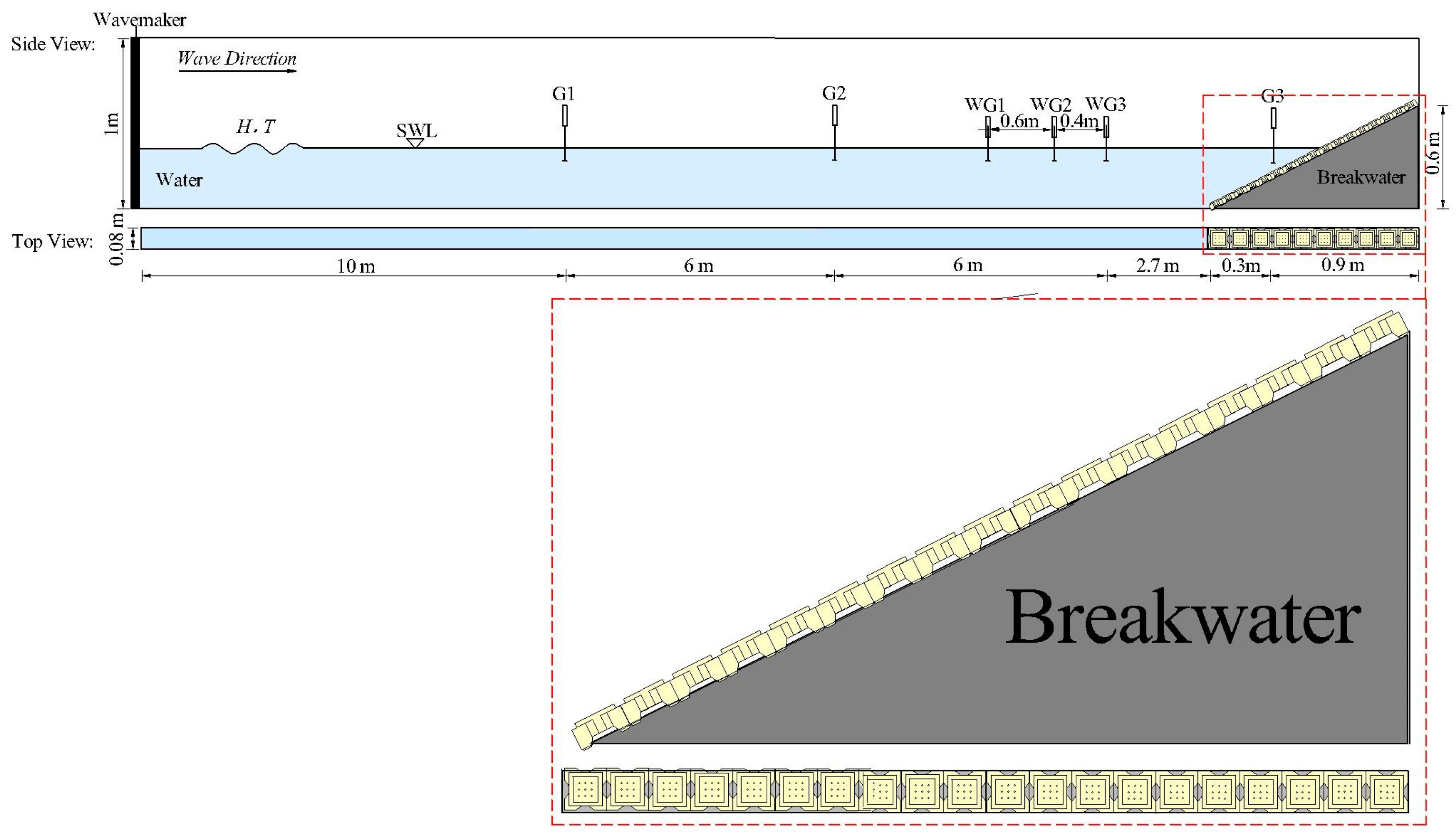
3.1. The New Ecological Hollow Cube

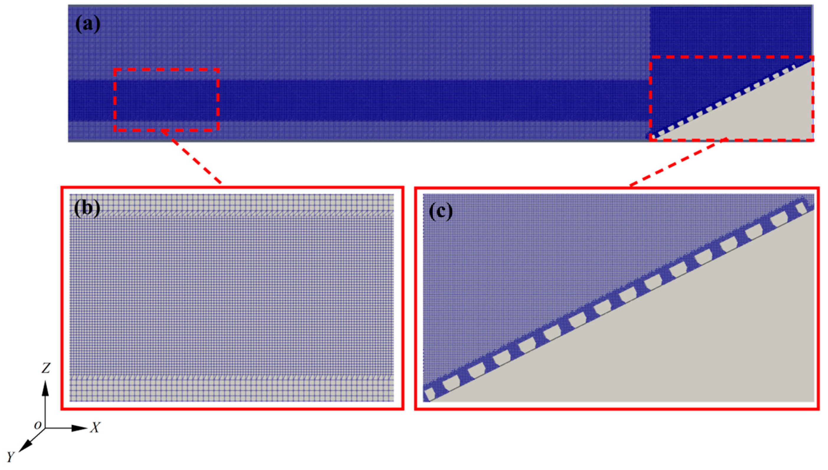
The new ecological hollow cube is transformed from the traditional hollow cube. On the basis of traditional hollow cubes with a raised frame and appropriate digging down to form a planting groove, nine cavities are arranged in the planting groove for wave dissipation. The geometry and dimensions of the block are visually presented in Figure 1. Its wave dissipation properties stem from the generation of turbulent vortices as waves enter the interconnected chambers within the block structure during their run-up on the slope. These vortices interact with the chamber walls, resulting in significant energy losses and effective wave attenuation. This new cube design provides a trifecta of advantages: high porosity, strong wave dissipation performance, and excellent structural stability, making it a promising solution for coastal protection.

3.2. Mesh

A three-dimensional numerical wave flume was designed, with the goal of accurately reproducing the experimental setup presented in Figure 2. To achieve this, the computational domain was configured with a length of 25.9 m, a height of 1 m, and a width of 0.08 m. The breakwater was positioned 24.7 m from the inlet boundary, mirroring the breakwater-wavemaker spacing in the experimental setup described by [2]. Three wave gauges (WG1, WG2, and WG3) used for incident wave analysis were defined at the exact locations used in the laboratory experiments. In addition, three wave gauges (G1, G2, and G3) were used in the numerical model to measure the wave surface changes. Nonslip boundary conditions were applied to all modeled impermeable structures, including the breakwater, cubes, and the flume bottom. At the atmospheric boundary, a fixed pressure was maintained, permitting bidirectional airflow while restricting water flow to an outflow condition only. The computational mesh was generated using blockMesh and snappyHexMesh, specifically for the breakwater and the cube structures. Within the OpenFOAM framework, blockMesh and snappyHexMesh are used as mesh generation tools. blockMesh was initially used to create the base mesh, considering the overall structure. Subsequently, snappyHexMesh was used to refine the mesh resolution in the vicinity of the free surface and around the cube structures.

A nonuniform mesh is used in the mesh generation process of the numerical model to simulate the wave propagation process effectively and the interaction between the wave and the structure. In Figure 3, the mesh near the water-air interface and around the structure was relatively dense, whereas the mesh in other areas was relatively loose. The number of meshes would be large (nearly 89 million grids would be needed to simulate the new ecological hollow cube in the experiment entirely) if the mesh around the armor block were generated on the basis of the configuration used in the physical modeling tests (flume width 0.8 m). Therefore, to simplify the calculations and improve computational efficiency, only one row of armored blocks was installed on the sloping breakwater, which is a numerical model that was fully verified in the study of [26]. Notably, Ref. [28] also used the one-row block method for their study and achieved good accuracy. The number of grids used in this study ranged from 891,844 (Mesh I), 2,922,119 (Mesh II), to 8,909,544 (Mesh III), from coarse to dense, respectively.

Table 2. Grid number and grid size in the computational domain.

Grid Information	Cell Number (Million)	Minimum Size in the x, y, and z Direction (m)
Mesh-I	891,844	0.005 × 0.005 × 0.005
Mesh-II	2,922,119	0.0025 × 0.0025 × 0.0025
Mesh-III	8,909,544	0.00125 × 0.00125 × 0.00125

provides an overview of the mesh characteristics, including the total cell count and the smallest grid spacing in each spatial dimension (x, y, and z) for the three different grid configurations used in this study.

Table 3. Wave conditions in the numerical simulation.

Test No.	Water Depth (m)	Period (s)	Wave Height (m)
Wave-I	0.3	2.46	0.08
Wave-II		1.79	0.06
Wave-III		1.12	0.04

shows the wave conditions used for the numerical studies.

3.3. Boundary Conditions

Inlet and outlet boundaries apply OlaFlow active generation and absorption boundaries. Non-slip velocity conditions are included for the flume bottom, blocks, and breakwater. The upper boundary, i.e., the atmosphere, is treated as an open boundary where water and air can leave the domain but only air may enter the domain again. The side boundaries are specified as periodic boundaries.

3.4. Post Processing of the Wave Run-Up and Reflection Coefficient

In Figure 2, three wave gauges, WG1, WG2, and WG3, were placed in front of a new ecological hollow cube to obtain reflection coefficients. In accordance with [29], the incident and reflected waves were separated. The proposed relationships are shown in Equations (18) and (19).

$$X_{12}={\displaystyle \frac{L_0}{10}}$$

(18)

$${\displaystyle \frac{L_0}{6}}< X_{13}< {\displaystyle \frac{L_0}{3}}\mathrm{and} X_{13}\ne {\displaystyle \frac{L_0}{5}}\mathrm{and} X_{13}\ne {\displaystyle \frac{3L_0}{10}}$$

(19)

where $X_{12}$ is the distance between wave gauges WG1 and WG2, $X_{13}$ is the distance between wave gauges WG1 and WG3, and L₀ is the shallow wavelength. According to the water depth at the breakwater, the wavelengths corresponding to different wave periods at different water levels are calculated via Equation (20).

$$L_0={\displaystyle \frac{g{T}^2}{2\pi }}\mathrm{t}\mathrm{a}\mathrm{n}\mathrm{h}(2\pi h/L)$$

(20)

In this study, wave reflection is quantified by the reflection coefficient C_r:

$$C_r={\displaystyle \frac{H_r}{H_i}}$$

(21)

where $H_i$ [m] and $H_r$ [m] are the incident and reflected wave heights, respectively.

In Figure 4, the wave run-up height was obtained by placing a plurality of probes near the surface of a new ecological hollow cube. Each probe is associated with a single computational cell, positioned at the cell’s centroid. The alpha water of the cell was recorded with each probe (alpha water indicates the percentage of water contained in the cell). For regular waves, the height of the run-up is usually expressed as R_u2%, defined as the height of the run-up exceeded by 2% of the incoming wave [30]. After analysis, the value of alpha water = 0.1 was used as the run-up height R_u2%. The probes with alpha water = 0.1 at all moments are counted, and the maximum value of the vertical coordinate of all the probes that satisfy the condition of the wave run-up height R_u2% is taken. For ease of understanding, R_u2% is denoted by R below.

4. The Results and Discussion

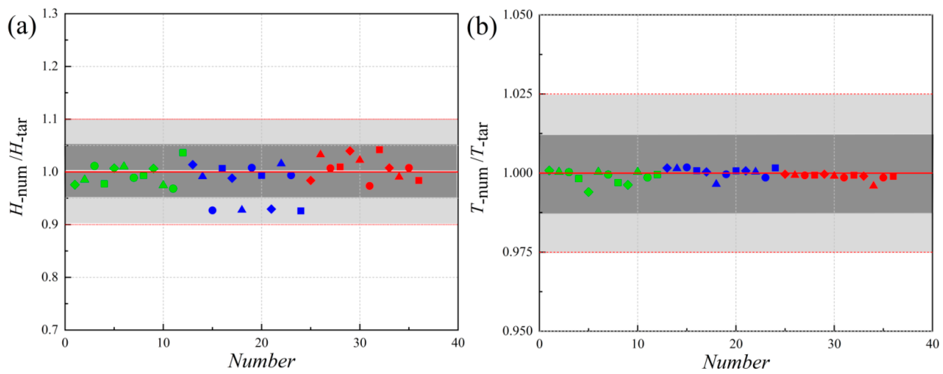
4.1. Wave Height and Period

In Figure 5, to validate the accuracy of numerical simulations, the numerically simulated wave features for all selected conditions were carefully compared with the corresponding target wave features. Figure 5b presents the results of the comparison between the numerically simulated and target wave periods, and it can be observed that there is a high degree of consistency between the two, which shows excellent agreement, and the quantitative metrics show that the mean absolute percentage error (MAPE) is only 0.68%. These findings indicate that the numerical model used in this study is highly reliable for wave height prediction. However, there are some deviations between the numerically simulated wave periods and the experimental measurements in Figure 5a. Specifically, the numerical model underestimates the wave heights with an average absolute error (MAPE) of 6.9%. The MAPE value is defined as follows:

$$\mathrm{M}\mathrm{A}\mathrm{P}\mathrm{E}={\displaystyle \frac{1}{n_{tests}}}\left({\displaystyle \frac{H_{tar}-H_{num}}{H_{tar}}}\right)\mathrm{*}100\mathrm{\%}$$

(22)

where $n_{test}$ is the number of tests on which the root mean square error (RMSE) is based. $H_{tar}$ is the target value, and $H_{num}$ represents the numerical value measured by the numerical model.

This error may be a run-up from the following aspects. First, the numerical model may fail to adequately capture the complex nonlinear effects or dissipation mechanisms in the wave propagation process, resulting in the wave energy not being correctly attenuated in the simulation. Second, the limitations of the grid resolution and the choice of the time step may also impact the wave period’s simulation accuracy. Therefore, although the numerical model exhibits satisfactory accuracy in wave period prediction, the prediction of wave height still needs to be further improved, and more refined numerical methods and parameter settings need to be explored in future studies to improve the overall simulation accuracy.

In Figure 5a, most data points fall in the dark gray region (within 5% error), indicating that all turbulence models better predict the incident wave heights. Overall, the performances of all the models in terms of incident wave heights are relatively close and show that the grid resolution has a small effect on the wave heights. In Figure 5b, most data points fall in the dark gray region (within a 1.25% error), indicating that all turbulence models predict the incident wave period more accurately, with little or no bias. The differences between different turbulence models (shapes) are negligible, and the differences between different grids (colors) are small, suggesting that the incident wave period is less sensitive to grid and model selection.

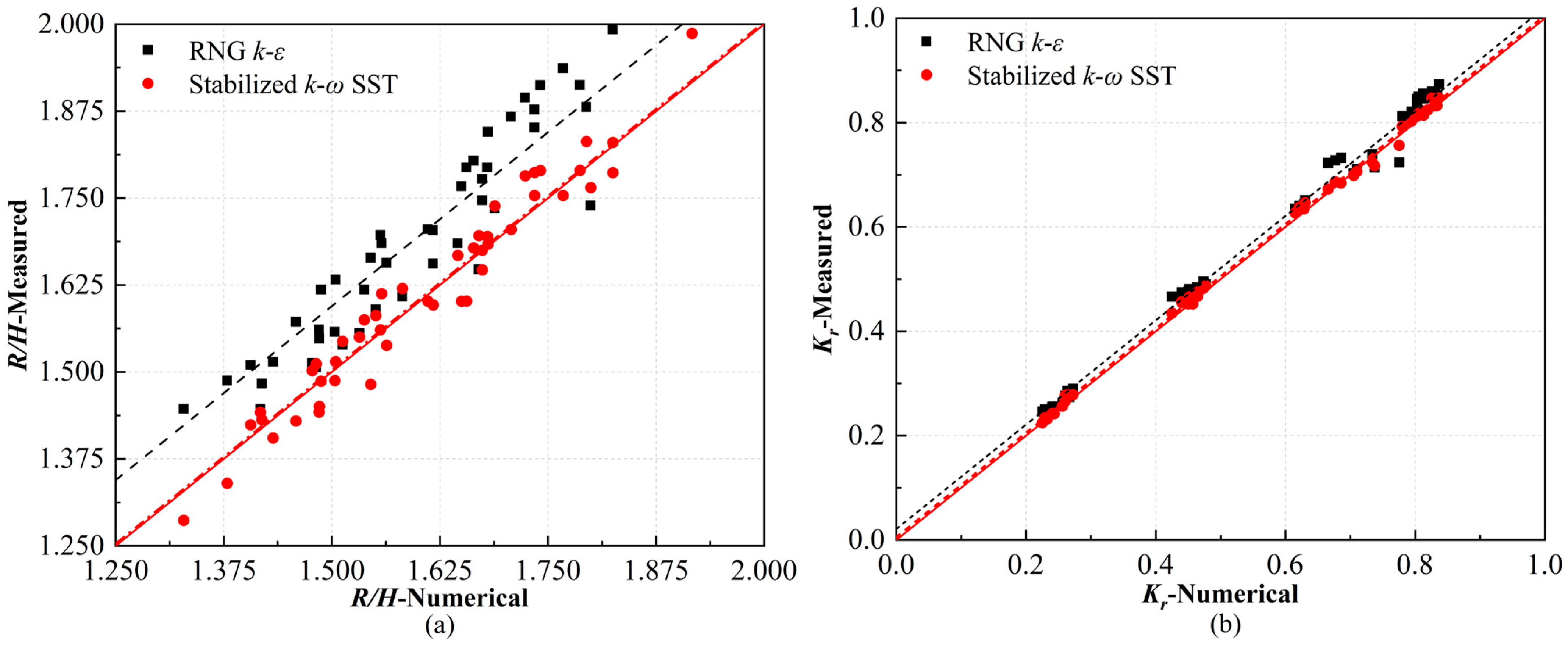
4.2. Validation of Numerical Model

The numerical model’s accuracy was assessed by comparing its predictions of wave run-up height and reflection coefficients against experimental data, focusing on a block structure under various incident wave conditions. Figure 6 presents the comparison, specifically detailing the results obtained using two turbulence models: the stabilized k-ω SST model and the RNG k-ε model. The simulations were conducted using Mesh II. Quantitative comparison reveals that the stabilized k-ω SST model yields more accurate results.

Figure 6a presents the “Wang et al. [26] (RNG k-ε)” data points (black squares) which are scattered around the diagonal line, but generally tend to overestimate the measured values (they lie above the diagonal line). The “Stabilized k-ω SST” data points (red circles) are generally below the diagonal, which means it is underestimating the R/H ratio. The root mean square error (RMSE) for wave run-up was 0.10914 for the stabilized k-ω SST model and 0.11114 for the RNG k-ε model. Figure 6b presents the both data sets (“Wang et al. [26] (RNG k-ε)” and “Stabilized k-ω SST”) which appear to be clustered much closer to the diagonal line, indicating better agreement between the numerical simulations and the measured data compared to Figure 6a. The data points are less scattered and more concentrated around the diagonal, suggesting higher accuracy in the numerical predictions for K_r. Similarly, the RMSE for wave reflection coefficients was 0.02109 for the stabilized k-ω SST model and 0.02799 for the RNG k-ε model. These values demonstrate that the numerical model, when implemented with the stabilized k-ω SST turbulence model, exhibits a better correlation with the experimental data, particularly in accurately predicting both wave run-up. Both models (RNG k-ε and stabilized k-ω SST) show very good agreement between the numerical and measured K_r values (Figure 6b). The choice of turbulence model (RNG k-ε and stabilized k-ω SST) has a greater impact on the accuracy of R/H ratio predictions than on K_r prediction.

4.3. Wave Profile Evolution

To obtain reliable numerical results, a comparative numerical modeling result under three different grid systems (Mesh I, Mesh II, and Mesh III) is performed, and three typical wave conditions (Wave-I, Wave-II, and Wave-III) are used. First, the time histories of the wave profiles at G1, G2, and G3 are comparatively analyzed under four different turbulence models (standard k-ε, stabilized k-ω SST, buoyancy-modified k-ω SST, and LES). G1 is located in the open sea in the fluid domain; G2 is in front of the breakwater; and G3 is in the front part of the breakwater. Notably, the wavefronts of the different turbulence models for both Wave-I and Wave-II conditions are very close to each other, so only the wavefronts of Wave-III are analyzed in this section (the RMSEs for Wave-I and Wave-II were 2.2154 × 10⁻⁵ and 6.16985 × 10⁻⁵, respectively). The numerical results using the standard k-ε, stabilized k-ω SST, buoyancy-modified k-ω SST, and LES turbulence models shown in Figure 7 indicate that there is significant nonlinearity after 30 s in the wave profile results at G1, G2, and G3 obtained via different grids. Overall, Figure 7 shows that the waves exhibit regular periodic fluctuations, and the results simulated with different grid densities are relatively close in most cases (the RMSE values for Mesh I and Mesh II, Mesh II and Mesh III are 6.13131 × 10⁻⁵, 6.56766 × 10⁻⁵, respectively), indicating good grid convergence. The wave profiles simulated with the standard k-ε, buoyancy-modified k-ω SST, and LES models show a slight decrease in wave height on three different grid systems (the RMSE values were 1.35112 × 10⁻⁵, 2.12065 × 10⁻⁵, 2.00269 × 10⁻⁵). In contrast, the wave profiles obtained with the stabilized k-ω SST model maintain good consistency (the RMSE value is 0.17832 × 10⁻⁵), with almost no wave height drop observed, suggesting better stability and grid independence under this condition.

To observe the numerical results under different turbulence models and grids more clearly, we select the time histories of the wave heights of G1, G2, and G3 in one period for comparison, focusing on evaluating their performance in capturing the free surface. In Figure 8, for Wave-I, the results of the standard k-ε model, the buoyancy-modified k-ω SST model, and the LES model are significantly correlated with the grid (the RMSE values for Mesh I and Mesh II are 6.13131 × 10⁻⁵, 6.56766 × 10⁻⁵, respectively). In contrast, the correlation of the stabilized k-ω model is not significant (the RMSE value for Mesh I and Mesh II is 3.91784 × 10⁻⁵). For both Wave-II and Wave-III, the grid dependence is insignificant for the stabilized k-ω model, standard k-ε model, buoyancy-modified k-ω SST model, and LES model. The stabilized k-ω model outperforms the standard k-ε model, the buoyancy-modified k-ω SST model, and the LES model in reliably capturing the free surface, which shows higher accuracy and reliability in simulating the wave free-surface flow.

4.4. Wave Run-Up

In practical engineering applications, wave run-up heights help in understanding the interaction between waves and structures. In addition, wave run-up heights are valuable for the placement and maintenance of critical infrastructure and for ensuring the safety of people in coastal areas. In

Table 4. Position of the probes.

Label	Coordinates (x, z, y) (cm)
P1	(x = 0.74525, z = 0.004, y = 0.40512)
P2	(x = 0.7515, z = 0.004, y = 0.40825)
P3	(x = 0.7565, z = 0.004, y = 0.41075)

, considering the influence of wave conditions on wave run-up heights, three groups of probes were designed in this study: P1, P2, and P3 (Figure 9). Therefore, a more accurate numerical model evaluation is achieved by selecting sounding points at different locations to ensure that sufficient variability data are available for different wave conditions.

This study examines the simulation results of different grids and turbulence models (standard k-ε, steady k-ω SST, buoyancy-modified k-ω SST, and LES) for wave run-up heights (alpha water) at each point from P1 to P3 under different wave conditions (Wave-I, Wave-II, and Wave-III) by comparing and analyzing the results. Under Wave-I and Wave-II conditions, the alpha water values of the grids are in good agreement overall (the RMSEs for Wave-I and Wave-II are 7.3621 × 10⁻⁵ and 8.7849 × 10⁻⁵, respectively). The results show that in Figure 10, under Wave-III conditions, the alpha water is more sensitive to the grids, and the models are less consistent among different grids, but all of them can capture the maximum value of alpha water better, among which the stable k-ω SST model can capture more alpha water values and shows a prediction advantage (the RMSE value of stable k-ω SST under Mesh I and Mesh II is 0.000362). However, there is an overestimation of the alpha water values in Mesh I at 25–35 s. Under Wave III conditions, the simulated alpha water values of Mesh I are generally higher than those of the other grids, especially the standard k-ε and LES models (the RMSE values of standard k-ε and LES models are 0.00166, 0.00125 for Mesh I and Mesh II, respectively), which are more significant. These findings emphasize the influence of grid resolution and turbulence model selection on the simulation results of wave run-up heights, particularly the dominance of the stabilized k-ω SST model in predicting alpha water.

To analyze the effects of different turbulence models, wave conditions, and grid resolutions on the wave run-up height in detail, the time histories of one cycle at each measurement point from P1 to P3 are selected for comparison in this study. In Figure 11, all four turbulence models exhibit significant grid dependence under different wave conditions, and this dependence is more significant the farther the measurement point P is from the structure. However, the consistency of the alpha water content over time is poor under different models and conditions, especially when the measurement point P is farther from the structure (e.g., P3). Overall, the alpha water parameter is more sensitive to the grid in the wave run-up calculation. The difference in the results between different turbulence models is not apparent. However, the results are related to the location of the measurement point: the closer the measurement point is to the structure, the smaller the dependence of the results on the grid, and vice versa, the dependence increases, which indicates that the effects of the turbulence model, the grid resolution, and the location of the measurement point need to be considered comprehensively in simulating the height of the wave run-up.

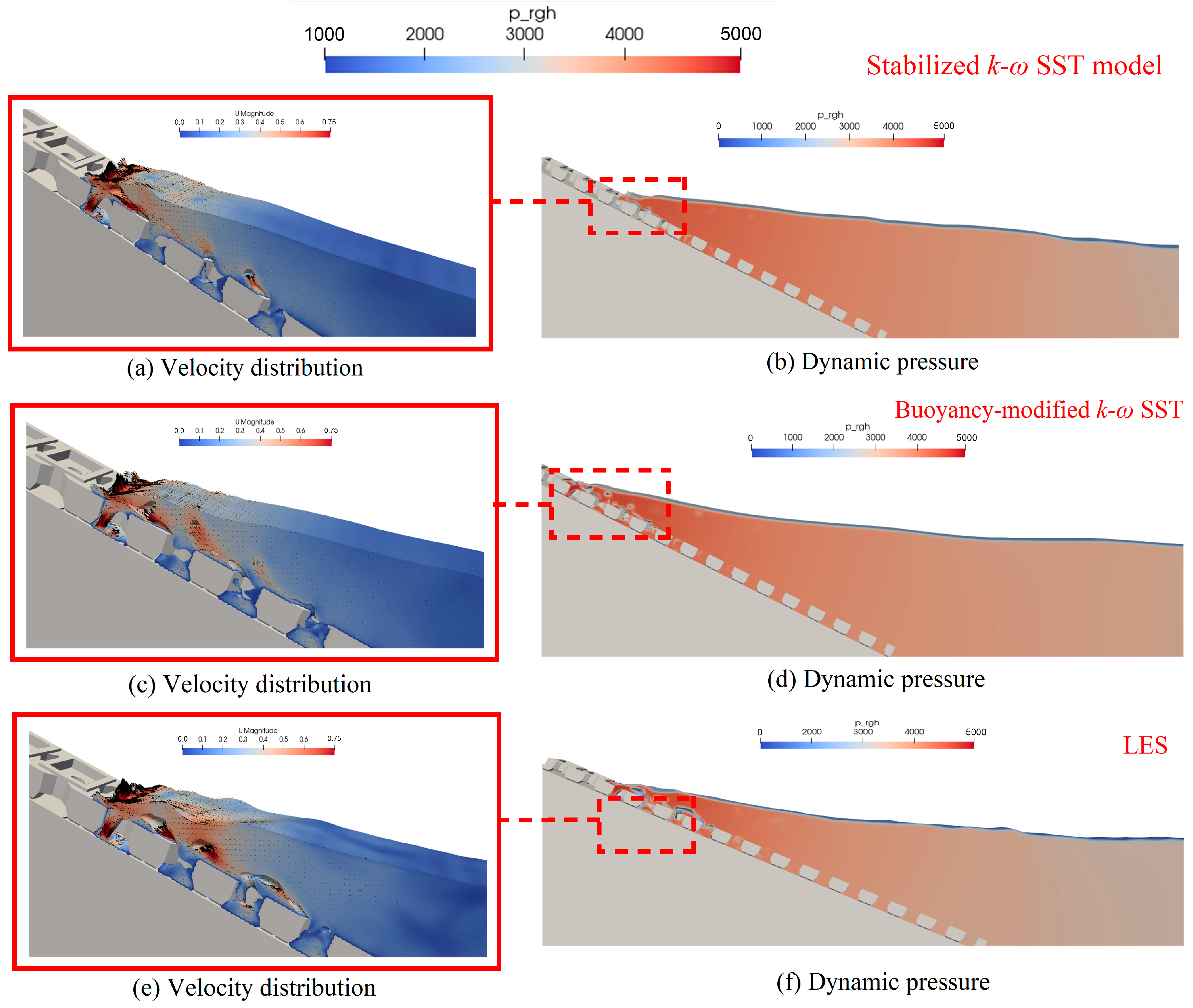
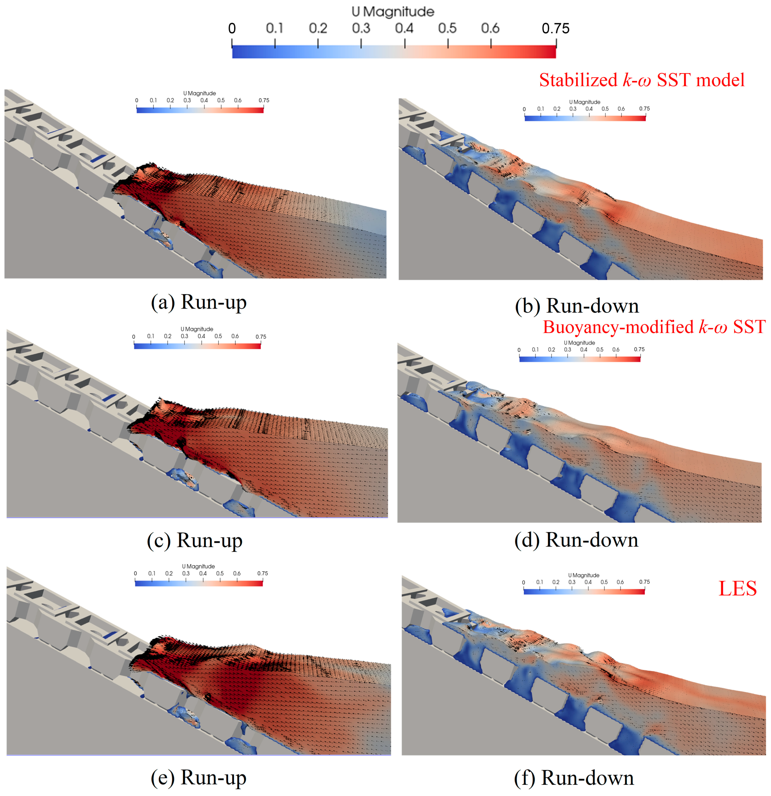
4.5. Wave Velocity Distribution and Dynamic Pressure Fields

Figure 12 shows the velocity distributions and pressure fields of different turbulence models (stabilized k-ω SST, standard k-ε, buoyancy-modified k-ω SST, and LES) on the new ecological hollow cube under Mesh III. Since the velocity distribution and pressure field of steady k-ω SST and standard k-ε are very close to each other, only the velocity distribution and pressure field plots of steady k-ω SST are given in Figure 12. The results show that the pressure fields of all four models tend to increase in pressure near the cube, and the overall pressures of the stabilized k-ω SST and buoyancy-modified k-ω SST models are slightly greater than those of the other models in terms of the velocity distribution. The stable k-ω SST and standard k-ε models behave similarly. Tiny vortices are present on the surface of the wave block and the front of the wave concentrate velocities. The k-ω SST model shows smaller eddies and velocities in the vicinity of the eddies. The LES model exhibits more pronounced wave surface undulations, reflecting the excessive generation of turbulent kinetic energy. This latter reflection leads to wave energy attenuation affecting in turn the wave surface and wave motion. The stabilized k-ω SST, standard k-ε, and buoyancy-modified k-ω SST models can better solve the problem of turbulent kinetic energy generation and produce a smoother free surface.

The velocity distributions and pressure fields of different turbulence models (stabilized k-ω SST, standard k-ε, buoyancy-modified k-ω SST, and LES) on the new ecological hollow cube under Mesh III are shown in Figure 13. The results show that the velocities of the stabilized k-ω SST and standard k-ε models are mainly concentrated on the surface of the new ecological hollow cube during wave run-up. In the wave run-down phase, the four models have similar characteristics. However, the free-surface velocity distributions of the stabilized k-ω SST and standard k-ε models are larger. In comparison, the velocity distributions of the buoyancy-modified k-ω SST model are smaller and smoother. In contrast, the LES model has a larger free-surface velocity distribution and more dramatic surface undulations. Overall, the free-surface velocity distributions of the stabilized k-ω SST model are very close to those of the standard k-ε model in the wave run-up and run-down phases. The buoyancy-modified k-ω SST model has the most minor and smoothest free-surface velocity distributions. The suggest that the different turbulence models present different flow field characteristics when simulating free-surface flows.

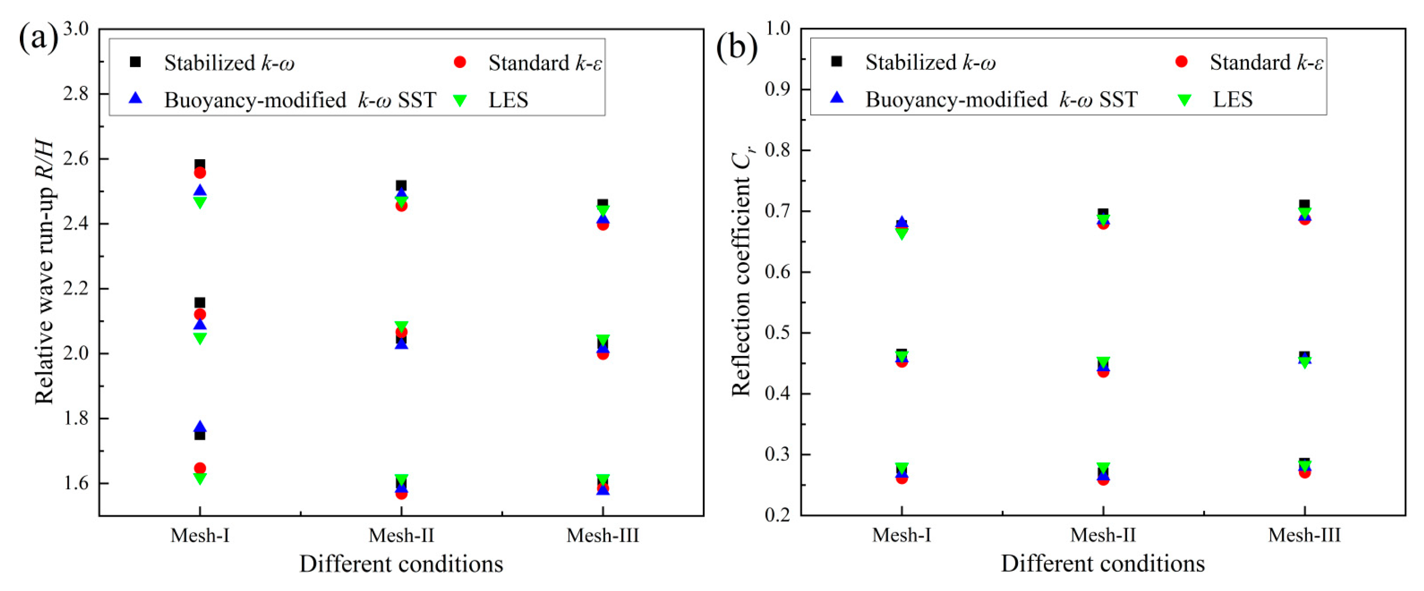
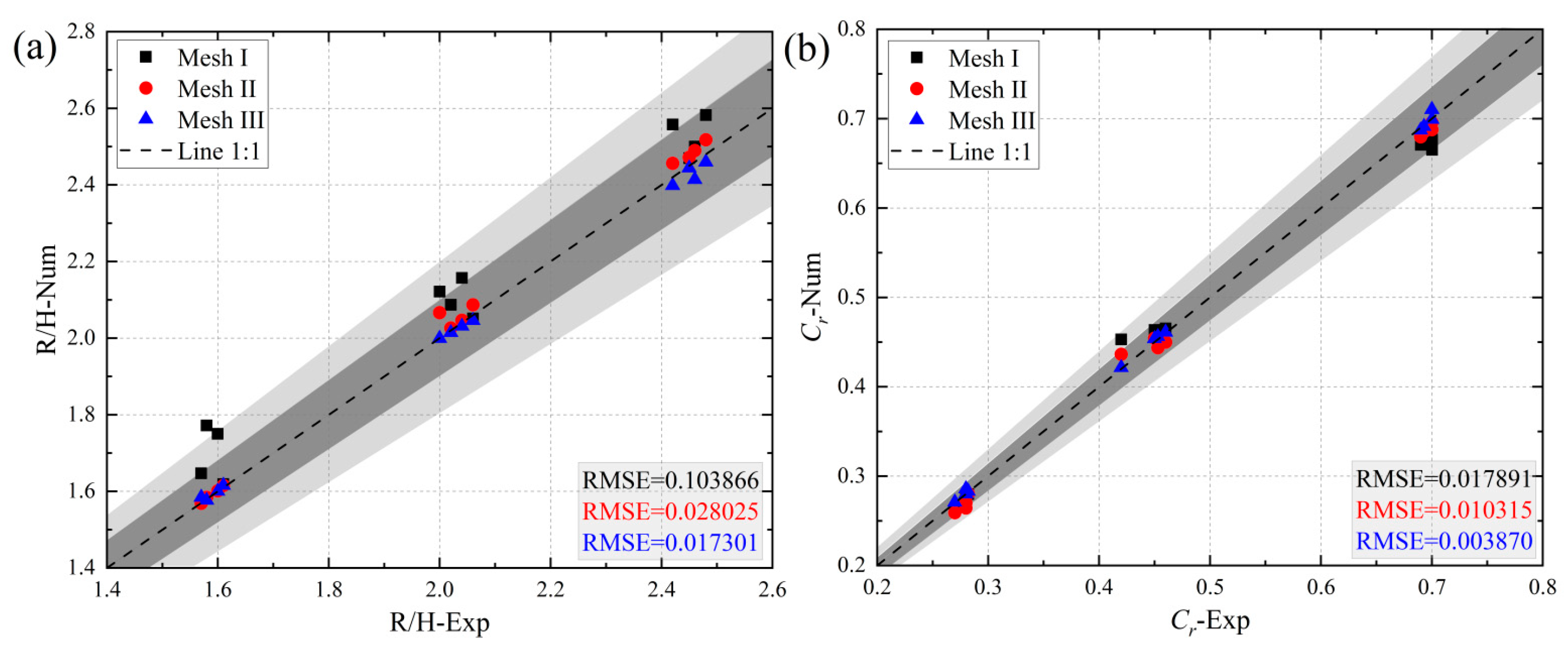
4.6. Sensitivity Analysis of the Wave Run-Up and Reflection Coefficient

In order to assess the influence of grid resolution on the numerical solutions, the extrapolated relative error (ERE) and grid convergence index (GCI) were computed to quantify the discretization error [31]. In this context, ‘s’ denotes the characteristic grid size for the numerical model:

$$s={[{\displaystyle \frac{1}{N}}{\sum }_{i=1}^N(\Delta V_i)]}^{0.5}$$

(23)

where ΔV_i is the volume of the ith cell and N is the total number of cells.

For the grid independence study, three different grid resolutions were implemented at the free surface: s₁ = 0.005 m, s₂ = 0.0025 m, and s₃ = 0.00125 m. Here, ‘s’ denotes the grid size, and the subscripts 1, 2, and 3 correspond to grid partition schemes Mesh I, Mesh II, and Mesh III, respectively.

The GCI is defined as follows:

$${GCI}_{21}={\displaystyle \frac{1.25e_{21}}{r_{21}^n-1}}$$

(24)

where

$$e_{21}=\left|{\displaystyle \frac{{\Psi }_1-{\Psi }_2}{{\Psi }_1}}\right|$$

(25)

$$n={\displaystyle \frac{1}{ln{r}_{21}}}\left|\ln \left({\delta }_{32}/{\delta }_{21}\right)+q\left(n\right)\right|$$

(26)

$$q(n)=\mathrm{l}\mathrm{n}({\displaystyle \frac{r_{21}^n-p^{\prime }}{r_{32}^n-p^{\prime }}})$$

(27)

$$p^{\prime }=Sign({\delta }_{32}/{\delta }_{21})$$

(28)

Here,${\delta }_{32}$ = ${\Psi }_3$ − ${\Psi }_1$, ${\delta }_{21}$ = ${\Psi }_2$ − ${\Psi }_1$, $r_{21}$ = $s_2$/$s_1$, and $r_{32}$ = $s_3$/$s_2$. The variable $\Psi$ represents the numerical solution obtained on a given grid. The function “Sign” refers to the sign function. Based on these definitions, the solution is expected to demonstrate either monotone convergence or divergence when $p^{\prime }$ = 1, and oscillatory convergence when $p^{\prime }$ = −1.

The extrapolated value is

$${\Psi }_{ext}^{21}=\left(r_{21}^n{\Psi }_1-{\Psi }_2\right)/(r_{21}^n-1)$$

(29)

Moreover, the ERE is

$${ERE}_{21}=\left|{\displaystyle \frac{{\Psi }_{ext}^{21}-{\Psi }_1}{{\Psi }_{ext}^{21}}}\right|$$

(30)

Table 5. Analysis of the discretization error.

Type	Partition Scheme	Values	Wave-I	Wave-II	Wave-III
Standard k-ε	Mesh I	R/H	1.75000	1.60125	1.57000
		Cr	0.27773	0.26991	0.28575
	Mesh II	R/H	2.15667	2.04667	2.03125
		Cr	0.46507	0.44991	0.461
	Mesh III	R/H	2.58219	2.51781	2.45969
		Cr	0.67653	0.69569	0.71023
	${\Psi }_{ext}^{21}$	R/H	−7.02350	−6.11255	−4.45310
		Cr	−1.17734	−0.22264	−0.12940
	${ERE}_{21}$	R/H	1.25%	1.26%	1.35%
		Cr	1.24%	2.21%	3.20%
	${GCI}_{21}$	R/H	6.27%	6.02%	4.80%
		Cr	6.55%	2.28%	1.82%
Stabilized k-ω SST	Mesh I	R/H	1.64688	1.56875	1.58438
		Cr	0.26136	0.25905	0.27081
	Mesh II	R/H	2.12125	2.06667	1.95933
		Cr	0.45292	0.43634	0.431241
	Mesh III	R/H	2.5575	2.45625	2.39813
		Cr	0.67056	0.6798	0.68706
	${\Psi }_{ext}^{21}$	R/H	−3.78187	−0.22172	−0.61746
		Cr	−1.14567	−0.21597	0.05407
	${ERE}_{21}$	R/H	1.44%	8.08%	3.57%
		Cr	1.23%	2.20%	4.16%
	${GCI}_{21}$	R/H	4.12%	1.43%	1.74%
		Cr	6.73%	2.29%	1.01%
Buoyancy-modified k-ω SST	Mesh I	R/H	1.58438	1.57688	1.77188
		Cr	0.26432	0.28003	0.26852
	Mesh II	R/H	2.02667	2.01458	2.08667
		Cr	0.44362	0.45617	0.4583
	Mesh III	R/H	2.48969	2.41406	2.49975
		Cr	0.68529	0.69106	0.68056
	${\Psi }_{ext}^{21}$	R/H	−0.84036	−0.25113	−0.24806
		Cr	−7.85221	−2.99801	0.76371
	${ERE}_{21}$	R/H	1.32%	2.05%	2.13%
		Cr	1.20%	1.53%	1.32%
	${GCI}_{21}$	R/H	5.16%	2.44%	2.36%
		Cr	7.45%	3.63%	0.71%
LES	Mesh I	R/H	1.61875	1.61563	1.61563
		Cr	0.27988	0.28047	0.28308
	Mesh II	R/H	2.05125	2.08708	2.04583
		Cr	0.46338	0.45438	0.45369
	Mesh III	R/H	2.46969	2.47188	2.44406
		Cr	0.665	0.6878	0.6991
	${\Psi }_{ext}^{21}$	R/H	−11.25289	−3.74310	−0.47801
		Cr	−1.57841	−0.22776	−0.10606
	${ERE}_{21}$	R/H	1.14%	1.43%	4.38%
		Cr	1.18%	2.23%	3.67%
	${GCI}_{21}$	R/H	9.94%	4.15%	1.62%
		Cr	8.30%	2.27%	1.72%

shows in detail the discretization errors of the relative wave run-up and reflection coefficients of the new ecological hollow cube for three different wave conditions (Wave-I, Wave-II, and Wave-III) as well as for four turbulence models (e.g., standard k-ε, stabilized k-ω SST, buoyancy-modified k-ω SST, and LES). The results show that the discretization errors for the four turbulence models exhibit a high degree of consistency across the three wave conditions: the highest error values are generally found in the Wave-I condition, whereas the lowest values are found in the Wave-III condition. This trend suggests that wave conditions significantly impact the accuracy of numerical simulations, with Wave-I representing the most complex wave dynamics scenario, leading to large uncertainties in model predictions. The stabilized k-ω SST turbulence model exhibits relatively better performance in terms of discretization error, and its predictions are in better agreement with the experimental data. These results suggest that the stabilized k-ω SST model may be a more robust and efficient choice for wave interaction simulations for this type of ecological hollow cube. However, other turbulence models may also exhibit acceptable accuracy in specific cases. To evaluate the performance of each turbulence model more comprehensively, it still needs to be considered in conjunction with other factors (e.g., computational cost and model robustness) and further explored in subsequent studies.

To better understand wave run-up, wave reflection coefficients are important because wave reflection affects the sea state and can impede safe navigation [32]. In addition, increased scour due to a high reflection coefficient can affect the stability of coastal structures [33]. Figure 14 shows the relative wave run-up and reflection coefficients when different turbulence models are used. Under the same wave conditions, the relative wave run-up heights derived from the four different turbulence models increase with decreasing grid size, and the reflection coefficient decreases with decreasing grid size. The differences in the wave rise heights and reflection coefficients for different grids are shown in Figure 15, which reveals that the wave run-up height and reflection coefficient of the new ecological hollow cube have some grid dependence. The RMSE value is defined as follows:

$$\mathrm{R}\mathrm{M}\mathrm{S}\mathrm{E}=\sqrt{{\displaystyle \frac{{\sum }_{i=1}^{n_{tests}}(K_{measured}-K_{numerical}{)}^2}{n_{tests}}}}$$

(31)

where $n_{test}$ represents the number of experimental or simulation runs used to calculate the root mean square error (RMSE). $K_{measured}$ is the experimentally measured value, and $K_{numerical}$ represents the numerical value measured by the numerical model.

Wave run-up and reflection have been extensively studied through both experimental and numerical approaches [34]. However, few works have discussed the grid sensitivity of wave run-up and reflection coefficients. Therefore, the comparative analysis of the wave run-up height and reflection coefficients of the new ecological hollow cubes with different turbulence models for different grid systems derived in this section is informative. Moreover, turbulence models that are not available in this study or more precise grid sizes can be used for further research to obtain more credible results.

5. Conclusions

This study presents a comparative analysis of hydrodynamic modeling of the new ecological hollow cube, utilizing the open-source solver olaFlow as the computational platform, with three mesh systems and four RANS turbulence models. The characteristics of wave evolution on the new ecological hollow cube, including wave run-up, velocity distribution, pressure fields, and reflection coefficients, were comprehensively compared. The key findings of this study are summarized as follows:

(1)

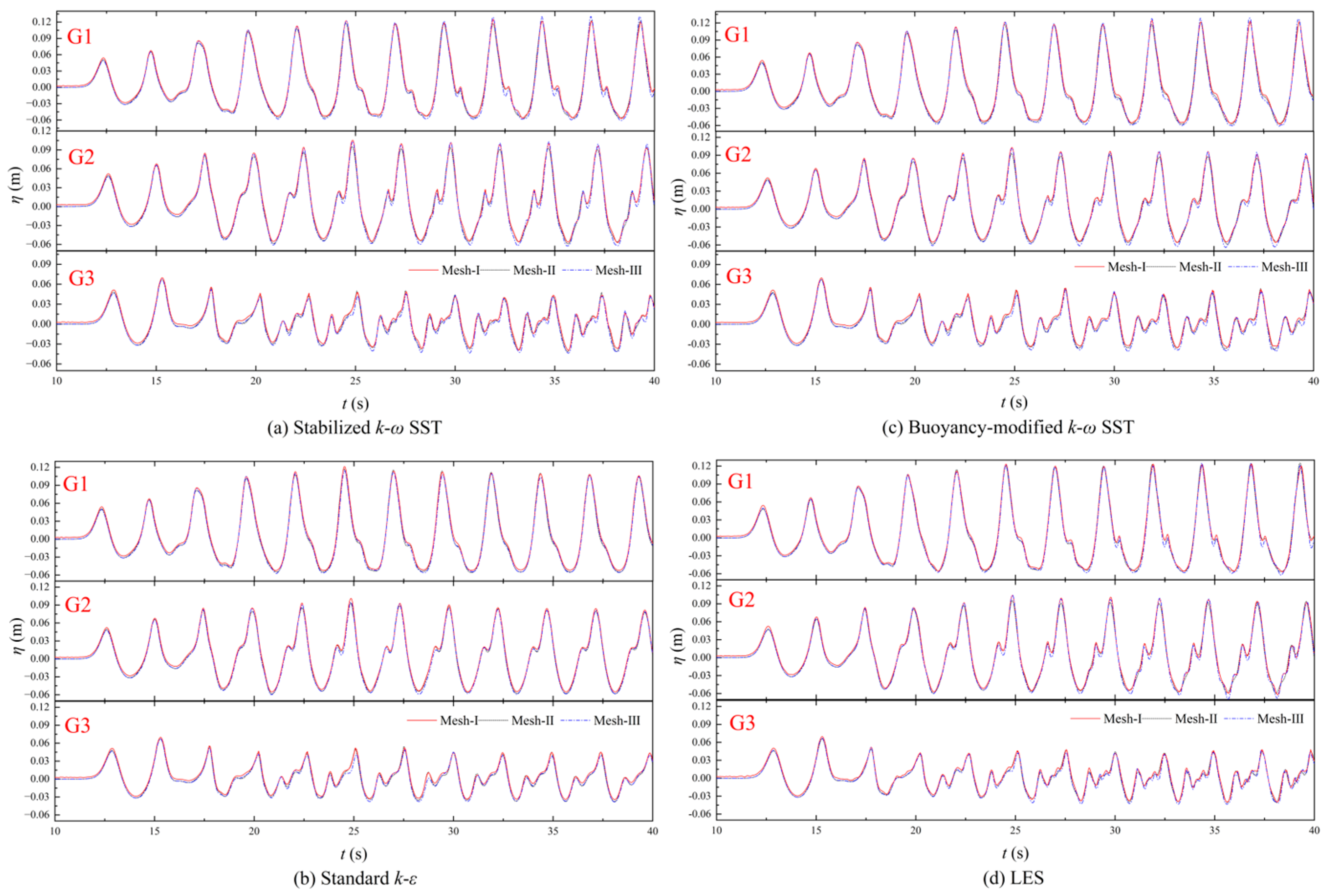
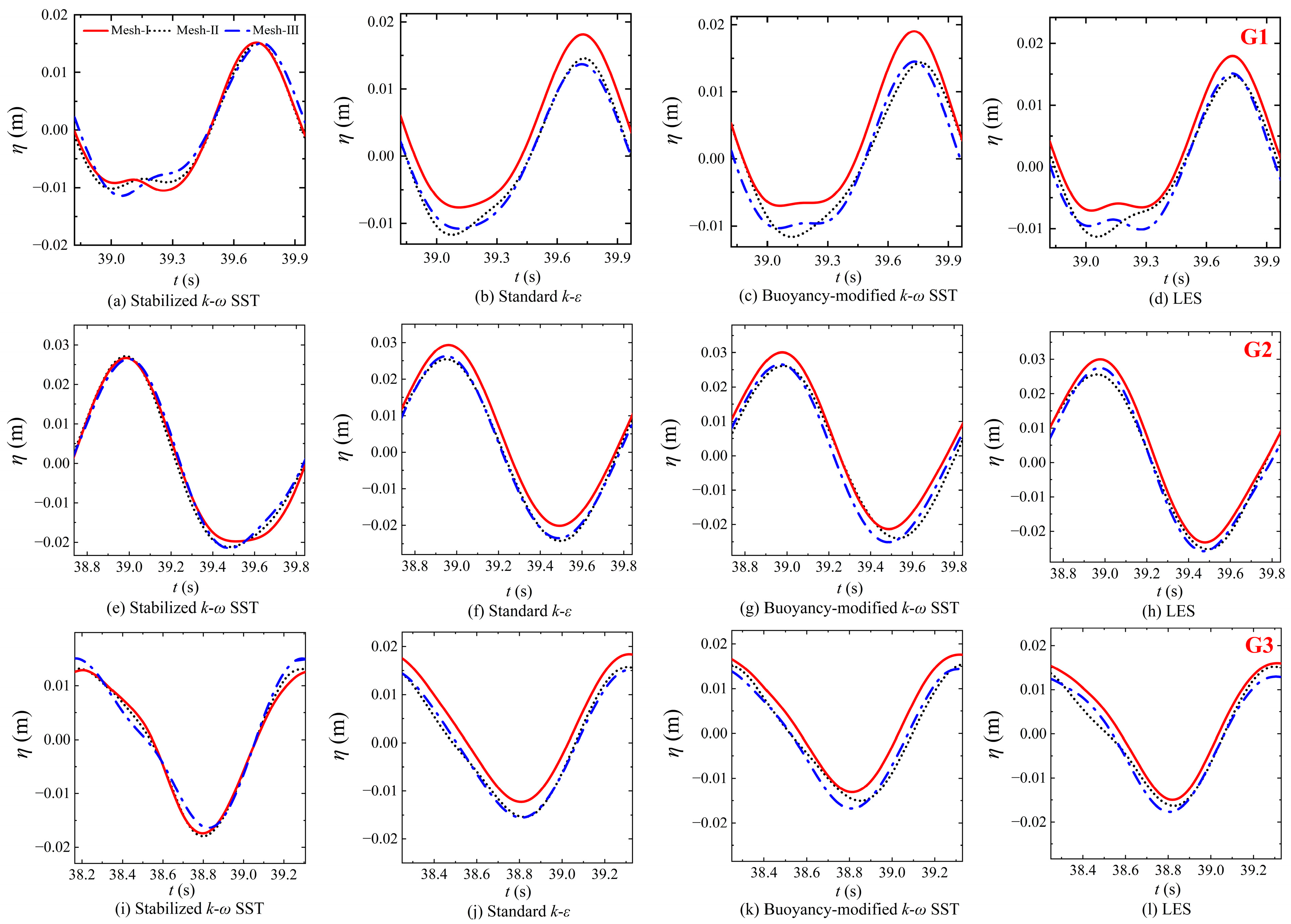
The stabilized k-ω model demonstrates superior performance in capturing wave evolution on the new ecological hollow cube. The wave profiles simulated with the standard k-ε, buoyancy-modified k-ω SST, and LES models show a slight decrease in wave height on three different grid systems (the RMSE values were 1.35112 × 10⁻⁵, 2.12065× 10⁻⁵, 2.00269 × 10⁻⁵). In contrast, the wave profiles obtained with the stabilized k-ω SST model maintain good consistency (the RMSE value is 0.17832 × 10⁻⁵), with almost no wave height drop observed, suggesting better stability and grid independence under this condition.

(2)

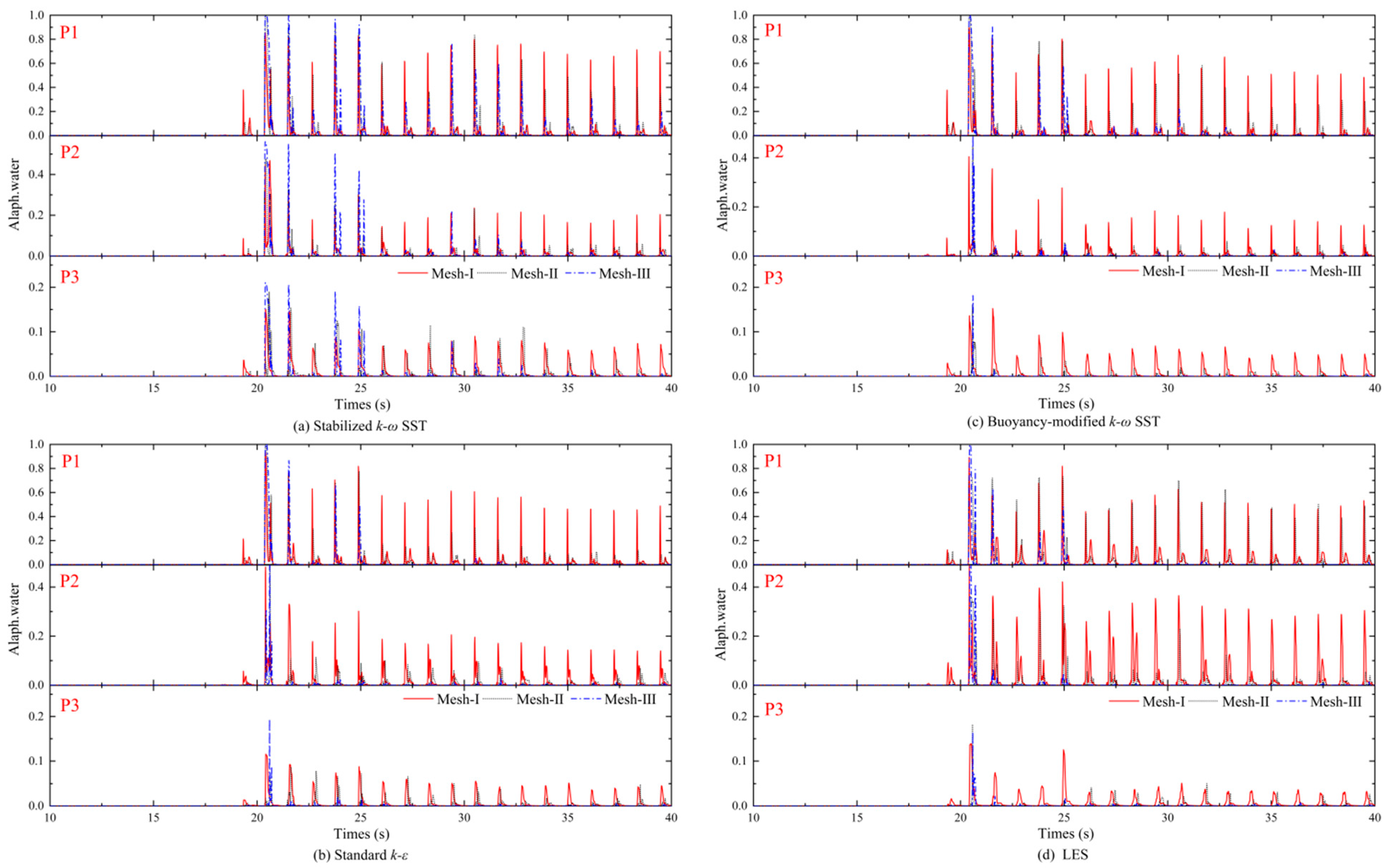
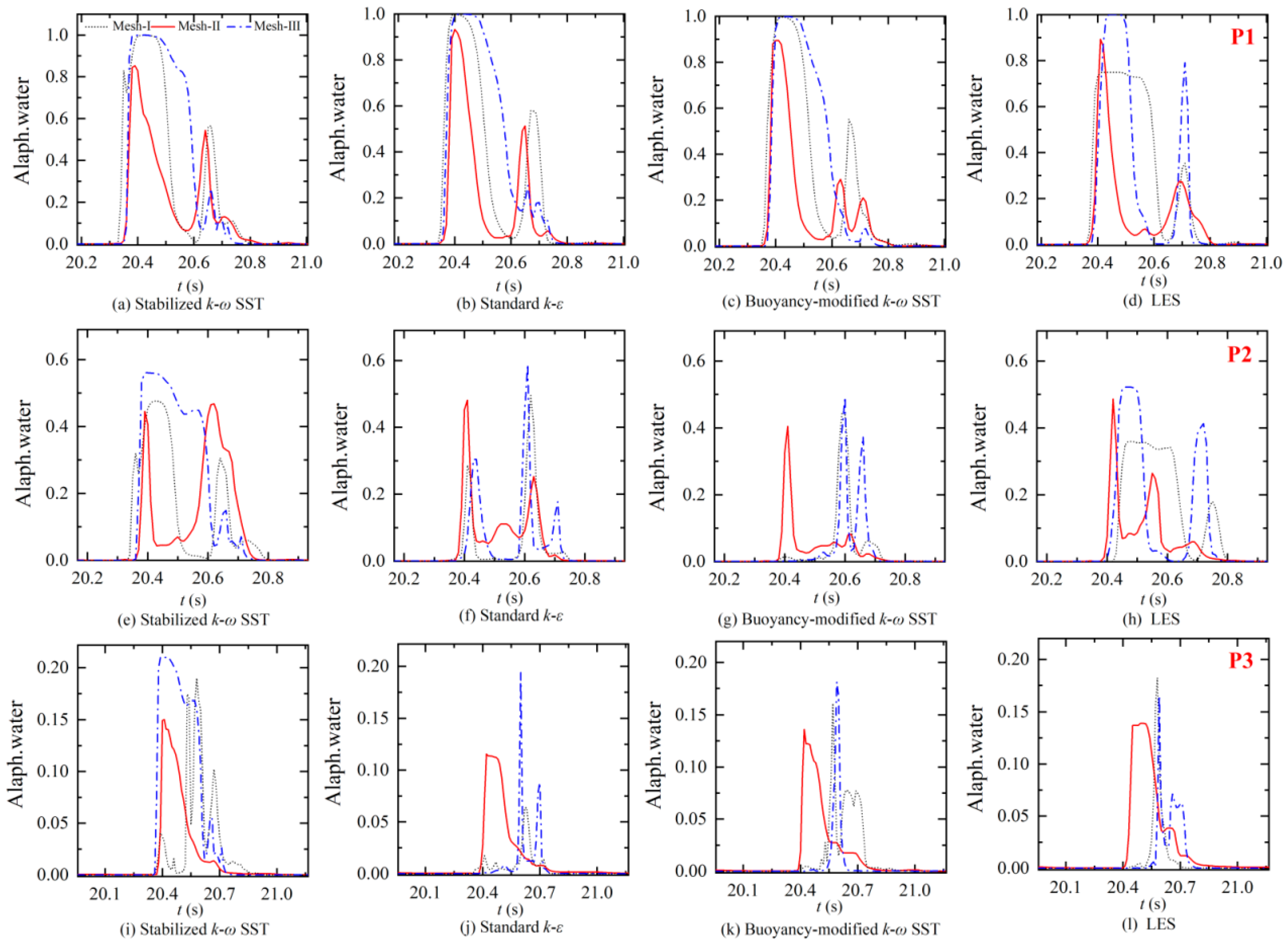
The parameter “alpha water” is more sensitive to the grids, and the models are less consistent among different grids, but all of them can capture the maximum value of alpha water better, among which the stable k-ω SST model can capture more alpha water values and shows a prediction advantage (the RMSE value of stable k-ω SST under Mesh I and Mesh II is 0.000362).

(3)

The pressure fields predicted by all four turbulence models are generally similar, with higher pressures observed near the new ecological hollow cube. The stabilized k-ω and buoyancy-modified k-ω SST models predict slightly higher overall pressures compared to the standard k-ε and LES models. Regarding velocity distributions, the stabilized k-ω and standard k-ε models show very similar patterns. The LES model, however, exhibits excessive turbulent kinetic energy generation. The stabilized k-ω, standard k-ε, and buoyancy-modified k-ω SST models are better suited for mitigating this issue of excessive turbulence kinetic energy production, resulting in smoother free-surface representations.

(4)

The numerical results for the new ecological hollow cube exhibit some grid dependence. The analysis of discretization errors across the four turbulence models reveals a high degree of consistency across the three wave conditions. The highest error values are consistently observed under the Wave-I condition (the average GCI₂₁ values for wave run-up and reflection were 6.3725 and 7.2575, respectively), while the lowest error values are found under the Wave-III conditions (the average GCI₂₁ values for wave run-up and reflection were 2.63 and 1.315, respectively).

This study focused on numerical model calculations and corresponding physical model tests conducted under regular wave conditions. Future research should investigate the influence of irregular waves on cube performance. Additionally, this study employed a simplified slope breakwater and did not account for the complexities of breakwaters in real-world engineering scenarios. This aspect warrants further investigation in future work.

References

1. Bruce, T.; Van Der Meer, J.; Franco, L.; Pearson, J.M. Overtopping performance of different armour units for rubble mound breakwaters. Coast. Eng. 2009, 56, 166–179. [Google Scholar] [CrossRef]
2. Zhao, H.; Ding, F.; Ye, J.; Jiang, H.; Chen, W.; Gu, W.; Yu, G.; Li, Q. Physical Experimental Study on the Wave Reflection and Run-Up of a New Ecological Hollow Cube. J. Mar. Sci. Eng. 2024, 12, 664. [Google Scholar] [CrossRef]
3. Campos, Á.; Molina-Sanchez, R.; Castillo, C. Damage in rubble mound breakwaters. Part II: Review of the definition, parameterization, and measurement of damage. J. Mar. Sci. Eng. 2020, 8, 306. [Google Scholar] [CrossRef]
4. Spalart, P.; Allmaras, S. A one-equation turbulence model for aerodynamic flows. In Proceedings of the 30th Aerospace Sciences Meeting and Exhibit, Reno, NV, USA, 6–9 January 1992; p. 439. [Google Scholar]
5. Launder, B.E.; Spalding, D.B. The numerical computation of turbulent flows. In Numerical Prediction of Flow, Heat Transfer, Turbulence Combustion; Elsevier: Amsterdam, The Netherlands, 1983; pp. 96–116. [Google Scholar]
6. Yakhot, V.; Orszag, S.A.; Thangam, S.; Gatski, T.; Speziale, C. Development of turbulence models for shear flows by a double expansion technique. Phys. Fluids A Fluid Dyn. 1992, 4, 1510–1520. [Google Scholar] [CrossRef]
7. Wilcox, D.C. Reassessment of the scale-determining equation for advanced turbulence models. AIAA J. 1988, 26, 1299–1310. [Google Scholar] [CrossRef]
8. Menter, F.R. Two-equation eddy-viscosity turbulence models for engineering applications. AIAA J. 1994, 32, 1598–1605. [Google Scholar] [CrossRef]
9. Launder, B.E.; Reece, G.J.; Rodi, W. Progress in the development of a Reynolds-stress turbulence closure. J. Fluid Mech. 1975, 68, 537–566. [Google Scholar] [CrossRef]
10. Wilcox, D.C. Turbulence Modeling for CFD (Third Edition) (Hardcover); DCW Industries: La Canada, CA USA, 2006. [Google Scholar]
11. Smagorinsky, J. General circulation experiments with the primitive equations: I. The basic experiment. Mon. Weather. Rev. 1963, 91, 99–164. [Google Scholar] [CrossRef]
12. Brown, S.A.; Greaves, D.M.; Magar, V.; Conley, D.C. Evaluation of turbulence closure models under spilling and plunging breakers in the surf zone. Coast. Eng. 2016, 114, 177–193. [Google Scholar] [CrossRef]
13. Mayer, S.; Madsen, P.A. Simulation of breaking waves in the surf zone using a Navier-Stokes solver. Coast. Eng. 2001, 2000, 928–941. [Google Scholar]
14. Devolder, B.; Troch, P.; Rauwoens, P. Performance of a buoyancy-modified k-ω and k-ω SST turbulence model for simulating wave breaking under regular waves using OpenFOAM®. Coast. Eng. 2018, 138, 49–65. [Google Scholar] [CrossRef]
15. Devolder, B.; Rauwoens, P.; Troch, P. Application of a buoyancy-modified k-ω SST turbulence model to simulate wave run-up around a monopile subjected to regular waves using OpenFOAM®. Coast. Eng. 2017, 125, 81–94. [Google Scholar] [CrossRef]
16. Larsen, B.E.; Fuhrman, D.R.; Roenby, J. Performance of interFoam on the simulation of progressive waves. Coast. Eng. J. 2019, 61, 380–400. [Google Scholar] [CrossRef]
17. Bradford, S.F. Numerical simulation of surf zone dynamics. J. Waterw. Port Coast. Ocean. Eng. 2000, 126, 1–13. [Google Scholar] [CrossRef]
18. Ting, F.C.; Kirby, J.T. Observation of undertow and turbulence in a laboratory surf zone. Coast. Eng. 1994, 24, 51–80. [Google Scholar] [CrossRef]
19. Galera-Calero, L.; Blanco, J.M.; Izquierdo, U.; Esteban, G.A. Performance assessment of three turbulence models validated through an experimental wave flume under different scenarios of wave generation. J. Mar. Sci. Eng. 2020, 8, 881. [Google Scholar] [CrossRef]
20. Qu, S.; Liu, S.; Ong, M.C. An evaluation of different RANS turbulence models for simulating breaking waves past a vertical cylinder. Ocean. Eng. 2021, 234, 109195. [Google Scholar] [CrossRef]
21. Zhou, H.; Ye, J. Numerical study on the hydrodynamic performance of a revetment breakwater in the South China Sea: A case study. Ocean. Eng. 2022, 256, 111497. [Google Scholar] [CrossRef]
22. Vieira, F.; Taveira-Pinto, F.; Rosa-Santos, P. Damage evolution in single-layer cube armoured breakwaters with a regular placement pattern. Coast. Eng. 2021, 169, 103943. [Google Scholar] [CrossRef]
23. Shen, Z.; Huang, D.; Wang, G.; Jin, F. Numerical study of wave interaction with armour layers using the resolved CFD-DEM coupling method. Coast. Eng. 2024, 187, 104421. [Google Scholar] [CrossRef]
24. Higuera, P.; Lara, J.L.; Losada, I.J. Three-dimensional interaction of waves and porous coastal structures using OpenFOAM®. Part I: Formulation and validation. Coast. Eng. 2014, 83, 243–258. [Google Scholar] [CrossRef]
25. Wang, Y.; Yin, Z.; Liu, Y. Numerical study of solitary wave interaction with a vegetated platform. Ocean. Eng. 2019, 192, 106561. [Google Scholar] [CrossRef]
26. Wang, Y.; Li, D.; Ye, J.; Zhao, H.; Mao, M.; Bai, F.; Hu, J.; Zhang, H. Numerical Analysis of Wave Interaction with a New Ecological Quadrangular Hollow Block. Water 2025, 17, 96. [Google Scholar] [CrossRef]
27. Yoshizawa, A.; Horiuti, K. A Statistically-Derived Subgrid-Scale Kinetic Energy Model for the Large-Eddy Simulation of Turbulent Flows. J. Phys. Soc. Jpn. 1985, 54, 2834–2839. [Google Scholar] [CrossRef]
28. Ye, J.; Shan, J.; Zhou, H.; Yan, N. Numerical modelling of the wave interaction with revetment breakwater built on reclaimed coral reef islands in the South China Sea—Experimental verification. Ocean. Eng. 2021, 235, 109325. [Google Scholar] [CrossRef]
29. Mansard, E.P.D.; Funke, E.R. The Measurement of Incident and Reflected Spectra Using a Least Squares Method. Coast. Eng. Proc. 1980, 1, 8. [Google Scholar] [CrossRef]
30. EurOtop. Manual on Wave Overtopping of Sea Defences and Related Structures, an Overtopping Manual Largely Based on European Research, But for Worldwide Application; Van der Meer, J.W., Allsop, N.W.H., Bruce, T., De Rouck, J., Kortenhaus, A., Pullen, T., Schüttrumpf, H., Troch, P., Zanuttigh, B., Eds.; 2018; Available online: https://www.overtopping-manual.com (accessed on 10 March 2025).
31. Celik, I.B.; Ghia, U.; Roache, P.J.; Freitas, C.J. Procedure for Estimation and Reporting of Uncertainty Due to Discretization in CFD Applications. J. Fluids Eng. 2008, 130, 078001. [Google Scholar]
32. Zanuttigh, B.; Van Der Meer, J. Wave reflection from coastal structures in design conditions. Coast. Eng. 2008, 55, 771–779. [Google Scholar] [CrossRef]
33. U.S. Army Corps of Engineers. Coastal Engineering Manual; U.S. Army Corps of Engineers: Washington, DC, USA, 2002; Volume 2.
34. Schoonees, T.; Kerpen, N.B.; Schlurmann, T. Full-scale experimental study on wave reflection and run-up at stepped revetments. Coast. Eng. 2022, 172, 104045. [Google Scholar] [CrossRef]
Figure 1. Schematic diagram of the new ecological hollow cube (unit: mm).
Water 17 01149 g001
Figure 2. Layout of the numerical wave flume.
Water 17 01149 g002
Figure 3. Mesh of the numerical wave flume: (a) side view, (b) free surface, (c) cube and breakwater.
Water 17 01149 g003
Figure 4. Probe to capture the wave run-up height.
Water 17 01149 g004
Figure 5. Comparisons of the numerical model and target incident height and period. (a) Incident wave height. The light gray areas depict the 10% error, and the dark gray areas depict the 5% error. (b) Incident wave period. The light gray areas depict the 2.5% error, and the dark gray areas depict the 1.25% error. The diamond, triangle, circle, and square markers represent the standard k-ε, stabilized k-ω SST, buoyancy-corrected k-ω SST, and LES, respectively. Green, blue, and red represent Mesh I, Mesh II, and Mesh III, respectively.
Water 17 01149 g005
Figure 6. Comparison of experimental and numerical wave run-up and reflections (stabilized k-ω SST and RNG k-ε). (a) Relative wave run-up; (b) reflection coefficients.
Water 17 01149 g006
Figure 7. Comparison of wave profiles at locations G1, G2, and G3 from numerical model test results under different turbulence models at Wave-III (third wave condition, Table 3).
Water 17 01149 g007
Figure 8. Comparison of wave profiles in one period when different turbulence models are adopted for Wave-II (second wave condition, Table 3).
Water 17 01149 g008
Figure 9. P1, P2, and P3 point maps.
Water 17 01149 g009
Figure 10. Comparison of alpha water on new ecological hollow cubes with different turbulent models under different grids in Wave-II (second wave condition, Table 3).
Water 17 01149 g010
Figure 11. Comparison of alpha water in one period with different turbulence models at P1, P2, and P3 during Wave-III (third wave condition, Table 3).
Water 17 01149 g011
Figure 12. Velocity distributions (left column, including (a,c,e)) and pressure fields (right column, including (b,d,f)) near the blocks (Wave-ⅠⅠⅠ, Mesh ⅠⅠⅠ).
Water 17 01149 g012
Figure 13. Run-up (left column, including (a,c,e)) and run-down (right column, including (b,d,f)) near the blocks (Wave-III, Mesh III).
Water 17 01149 g013
Figure 14. Comparison between the different mesh and turbulence models (a) R/H and (b) Cr.
Water 17 01149 g014
Figure 15. Comparison between the numerical and experimental (a) R/H and (b) Cr. The light gray areas depict the 30% error, and the dark gray areas depict the 15% error.
Water 17 01149 g015