Abstract
The offshore wind industry is increasingly moving towards larger turbines. The growth in rotor size and aerodynamic loads necessitates larger monopile foundations. This increased foundation height results in a monopile that exhibits pronounced slenderness and flexibility. Consequently, the fixed-bottom monopile becomes more susceptible to wave loads, which can induce nonlinear vibrations in complex wave environments. Extensive physical model experiments have been conducted in a wave tank to study the nonlinear vibration characteristics of a fixed-bottom monopile under regular wave action. The experimental results demonstrate that when the wave period is close to twice the resonant period of the model, the vibration response of the monopile increases significantly. Under these conditions, a second harmonic resonance occurs, with the amplitude of the second harmonic component being more than twice that of the fundamental (wave frequency) component. Additionally, the maximum run-up around the model exhibits a W-shaped distribution in the circumferential direction, with the highest run-up observed on the incident wave side. The wave pressure at the water surface is the greatest and increases with wave height, while the pressure below the water surface gradually increases with the measurement height.
1. Introduction
With the continuous growth in global energy demand, offshore wind power, as a clean and renewable energy source, has attracted widespread attention in recent years [1]. To reduce installation and maintenance costs, the offshore wind industry is transitioning towards larger turbines. The increase in rotor size and aerodynamic loads necessitates correspondingly larger support structures. Monopile support structures, due to their simple structure and low cost, have become the most widely used method for supporting offshore wind turbines [2]. In the context of wind turbines utilizing monopile support structures, an increase in the dimensions of the monopile support structure corresponds to a rise in both diameter and height. The monopile has the characteristics of height and flexibility [3]. Monopile-foundation offshore wind turbines are typically located in nearshore regions with water depths not exceeding 50 m [4]. Under the action of a complex ocean environment, it is easy to cause complex structural vibration of flexible monopile wind turbines [5]. The vibration exhibits remarkable nonlinear characteristics. This not only affects the safety of wind turbine installations but may also lead to structural fatigue and even severe issues such as turbine failure [6,7].
Hydrodynamic load is a major factor of vibration of wind turbines. Before studying the nonlinear vibration of wind turbines, many scholars pay attention to the hydrodynamic load of a monopile. By comparing experimental results with the diffraction theory solution, Morris-Thomas and Thiagarajan [8] concluded that long-wave theory can accurately predict the run-up of irregular waves on a vertical monopile. He conducted large-scale experiments, focusing on near-breaking and breaking waves. In contrast, Niedzwecki and Duggal [9] carried out small-scale experiments to study wave run-up on vertical cylinders and demonstrated that the linear assumption severely underestimates the wave crest heights around the cylinder under steep wave conditions. However, for offshore wind turbines, Marino et al. [10,11] emphasized the necessity of employing nonlinear wave kinematics when calculating hydrodynamic loads. This view is consistent with that of Paulsen et al. [12], who demonstrated, using CFD solvers, that the excitation forces computed based on linear wave kinematics do not contain the frequency components required to excite the structure’s first mode. Therefore, it is very important to consider the nonlinear effect of wave load on structural excitation.
Some researchers have already investigated the hydrodynamic response of rigid cylindrical wind turbine foundations subjected to wave loads. For example, Deng et al. [13] conducted numerical and experimental studies on the nonlinear wave loads and run-up on monopile foundations, employing a second-order potential flow model and a time domain higher-order boundary element method (HOBEM) to explore the nonlinear effects. Bredmose and Jacobsen [14] employed wave group focusing techniques to simulate extreme waves and studied the effects of breaking wave loads on a monopile, treated as a rigid structure. Ding et al. [15] studied the multidirectional and bidirectional wave interactions on monopile-supported offshore wind turbine foundations. Using a phase-based harmonic separation method, the harmonics under complex wave field conditions were successfully isolated. Under certain wave conditions, the nonlinear load accounted for up to 40% of the total load. Furthermore, wider wave propagation reduced the nonlinear higher-order harmonics, while unidirectional waves induced the most severe nonlinear forces. Sclavounos et al. [16] proposed an analytical model for predicting random nonlinear wave loads on both bottom-fixed and floating offshore wind turbine support structures, and based on Fluid Impact Theory (FIT), they derived an explicit expression for the time domain nonlinear excitation force under conditions where the wave height is comparable to the diameter of the support structure. Mockutė [17] calculated the loads on a rigid cylinder using both linear and nonlinear theories, and the results indicated that finite-depth FNV theory captures the broadest range of loads under wave–cylinder interaction. However, these studies have focused on rigid monopiles and have not fully considered the structural nonlinear vibrations induced by wave loads on monopile foundations. With the scaling up of monopile wind turbines, the monopile has increasingly exhibited pronounced slender and flexible characteristics. It is very important to study the impact of wave loads on nonlinear vibrations of the monopile.
Research on the effects of waves on flexible wind turbine structures has been carried out through both physical model experiments [18] and numerical simulations [19]. Ryan et al. [20] examined the impact of nonlinear wave loads on the response and design of the DTU 10 MW offshore wind turbine, supported by a monopile, under extreme conditions. Due to the coincidence of high harmonic loads with the natural period, the nonlinear model significantly influences the structural response. Jiang and Moctar [21] investigated the nonlinear effects of hydrodynamic loads on monopile-supported offshore wind turbines, with a particular focus on their harmonic structure. A novel four-phase decomposition technique was employed to effectively extract the harmonics from random time series, successfully isolating their fourth-order harmonic components. Harmonic analysis of wave elevation under different sea conditions indicated that the first harmonic is dominant, while the contribution of higher-order harmonics increases with wave steepness. However, notable differences were observed in the second harmonic. Wang et al. [22] analyzed the extreme loads on a 10 MW offshore monopile wind turbine under extreme sea conditions by coupling a nonlinear potential wave solver OceanWave3D with aero-elastic code HAWC2. The nonlinear waves significantly increased the extreme bending moments at the tower base and at the mudline of the monopile, primarily due to the resonance effects induced by wave nonlinearity. Bachynski et al. [23,24] investigated the response of monopile offshore wind turbines under irregular wave loads in various sea conditions and conducted full-flexible monopile model tests. The experimental results highlighted the resonance response of the monopile under severe wave loading, where the system’s first mode was predominantly excited by second-order and third-order wave loads. Furthermore, he developed a numerical analysis method for the flexible model, and the results indicated that as the natural frequency of the structure increases, the structural response decreases. In other words, a stiffer structure exhibits a smaller response. Suja-Thauvin et al. [25] studied the motion response of two bottom-fixed offshore wind turbines with monopile foundations in moderate water depths under severe irregular wave conditions. The first model was fully flexible, with its first and second characteristic frequencies and its first mode shape representing those of a full-scale turbine, and it was used to investigate the structural response. The second model was rigid and used to analyze the hydrodynamic excitation forces. The results showed that second- and third-order hydrodynamic loads induced a pronounced ringing response. Researchers from Denmark (DHI/DTU) also conducted wave tank tests on a flexible monopile foundation [26,27,28,29]. These tests were performed in a wave tank with a sloped bottom (1:25 scale) and covered regular waves, irregular waves, and focused breaking waves, including conditions representative of short-crested seas. Significant vibration responses were observed under steep and breaking wave conditions. Although the excitation was not explicitly identified as ringing, the results suggested that the responses induced by steep waves in both short-crested and long-crested sea states can be substantial. Suja-Thauvin et al. [30] further compared experimental data from a 4 MW monopile offshore model, tested under extreme irregular sea conditions in finite water depths, with numerical models used to evaluate Ultimate Limit State conditions in offshore wind standards. The model’s first and second characteristic frequencies, as well as its first mode shape, were adjusted to match those of a full-scale turbine. The mode that has the most significant impact on the model’s vibration is the first mode. The flexible models in the aforementioned studies all have multiple modes, and the movements between these modes interact with each other. This makes it difficult to independently study the impact of first-mode resonance on the model’s vibration. Bachynski et al. [31] used a rigid model with a leaf spring at the bottom to simulate the first mode of the monopile. However, the study primarily focused on the torque at the model’s base and did not emphasize the nonlinear vibration response of the model.
The aim of this paper is to establish a physical experiment model to simulate the first-order natural frequency of wind turbine structures more accurately. The second harmonic resonance of monopile-foundation wind turbines, caused by waves, is emphasized. The mechanism of wave force affecting the nonlinear vibration of the model is analyzed. The phenomena of wave run-up and dynamic response of the model are revealed. In this study, Section 2 presents the design of the scaled model and experimental conditions. Section 3 describes the experimental results and related discussions. Conclusions are drawn in Section 4.
2. Experimental Set-Ups
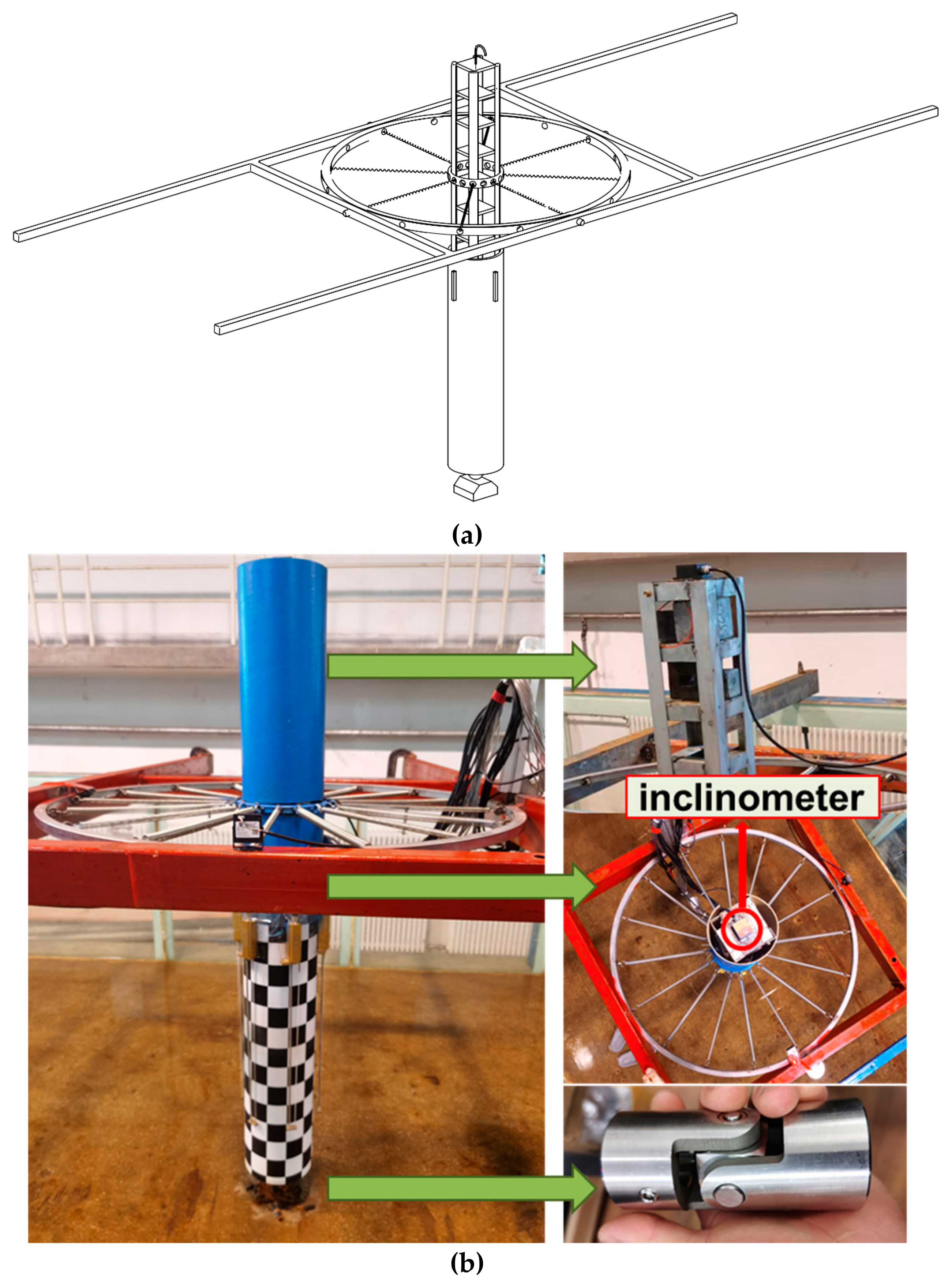
The physical model tank experiments were conducted in the Marine Environment Tank at the State Key Laboratory of Coastal and Offshore Engineering, Dalian University of Technology. The tank dimensions are 50.0 m in length, 3.0 m in width, and 1.0 m in height, with a maximum operating water depth of 0.7 m. Based on Froude similarity, a scaled model of the offshore wind turbine flexible support structure was designed and constructed at a 1:50 scale. The model operates at a water depth of h0 = 0.48 m. A monopile model with a diameter of 0.18 m was installed at the center of the tank, and the model has an overall height of 1.5 m. The model dimensions and corresponding full-scale parameters are provided in Table 1. The entire model is rigid, with a hinged lower part that provides flexibility. The overall installation of the physical model is shown in Figure 1.

Table 1.
Model-scale and full-scale dimensions.
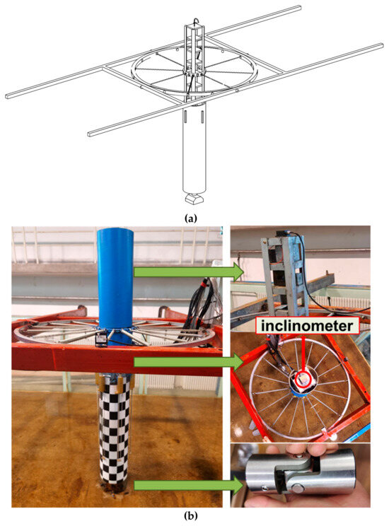
Figure 1.
Model test set-up of the experiments: (a) concept; (b) reality.
2.1. Model Description
The framework of the model was fabricated using stainless steel beams to provide the required high structural rigidity. This stainless steel framework ensures that the model maintains a stable support structure under wave action. To accurately adjust the center of mass and mass distribution of the wind turbine support structure, the model employed a concentrated mass unit array approach. Equidistantly spaced platforms, designed to accommodate ballast blocks, were welded onto the framework, thereby ensuring that the overall mass and the center of gravity of the model closely replicate those of the actual support structure. For the water-contacting portion, a cylindrical shell was used on the exterior of the model, ensuring that the dimensions of the cylindrical shell remain geometrically similar to the actual structure. This design guarantees that the wave loads acting on the model satisfy the dynamic similarity requirements relative to those experienced by the real wind turbine support structure. A universal joint connects the model’s base to the bottom of the water tank, enabling the model to achieve free fore–aft and lateral movement during the experiments.
At the upper part of the model, an annular arrangement of spring assemblies was installed. These spring groups are connected to a bracket fixed to the water tank wall, and by adjusting the number of springs, the natural frequencies of the model’s roll and pitch motions are calibrated to simulate the dynamic characteristics of various flexible support structures. The truss-type fixed frame is installed at the upper section of the water tank at the model’s location, spanning across both side walls. It possesses sufficient strength and rigidity to withstand the forces applied by the tension springs. Centrally mounted on this fixed frame is a circular ring with a diameter of 1.0 m. The function of the circular ring is to ensure that the connection between the springs and the model maintains a consistent initial length, thereby providing precise control throughout the experimental runs. The spring assembly, secured via the circular ring, guarantees the stability and uniformity of the force transmitted, while the opposite end of the springs is firmly connected to the model, ensuring that the model can move freely within the prescribed degrees of freedom.
2.2. Sensor Arrangement and Data Acquisition
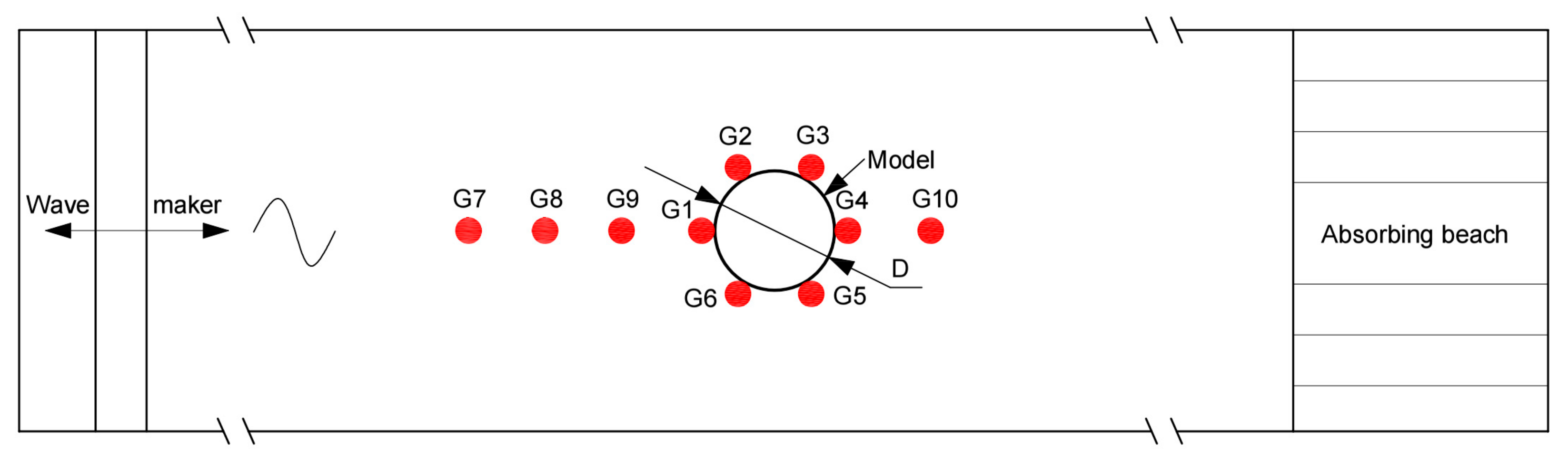
Six wave gauges were uniformly arranged around the model. Starting from the wave incident side, they were sequentially numbered G1 to G6 in a clockwise direction to record the time history of the waves near the model, as shown in Figure 2. The angular spacing between the adjacent gauges is 60°. Three wave gauges were placed in front of the model and one at the rear, numbered G7 to G10. Pressure sensors were installed on the wave incident side to measure the pressure acting on the model. The pressure sensors are evenly distributed at an interval of 0.02 m from 0.32 m to 0.64 m from the bottom of the water tank. The pressure sensors have an accuracy of 0.1% FS and a range of −10 kPa to 10 kPa. A high-precision inclinometer is installed on the top of the model to monitor the time history of the model’s angular displacement. This inclinometer is based on a high-performance, three-dimensional motion attitude measurement system using MEMS technology. It includes a three-axis gyroscope and a three-axis accelerometer, providing high-precision, high-dynamic, and real-time compensated three-axis attitude angles. The device can deliver data at an update rate of up to 200 Hz, enabling accurate motion capture and attitude estimation. The inclinometer’s measurement range is ±180° in the X-direction and ±90° in the Y-direction, with an angular accuracy of 0.05°. The sampling frequency of all measuring instruments is set at 100 Hz.
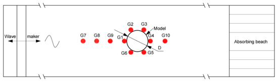
Figure 2.
Layout of gauges in the experiment.
2.3. Test Conditions
A wave maker was used to generate regular waves in the water tank. To investigate the effects of wave nonlinearity, experiments were conducted with 3 wave heights (H1 = 0.06 m, H2 = 0.09 m, H3 = 0.12 m) and 18 wave periods T for each height, resulting in a total of 54 test conditions (Table 2). According to the Froude similarity criterion, these conditions cover wave periods ranging from 3.5 s to 20.5 s, scaled to represent real-sea scenarios with full-scale wave heights of 3.0 m, 4.5 m, and 6.0 m. The wave length L was calculated for all test cases using the Stokes wave theory, , where h = 4.8 m is the water depth in the tank and H is the wave height. The calculated wave steepness ε = H/L values are explicitly listed in Table 2. According to Stokes wave theory, there exists a critical limit for this ratio, approximately 0.142 [13]. When the wave steepness exceeds this limit (εlim), wave breaking occurs. When a structure interacts with waves, the waves will break at a ratio smaller than εlim, which depends on the scale of the structure.
Table 2.
Tested wave conditions.
3. Results and Discussion
3.1. Free-Decay Text
Free-decay experiments were carried out in the wave tank to identify the natural pitch oscillation periods of the model. An initial disturbance is applied to the model in the pitch direction, and then the model is released. The model oscillates freely in the tank. The pitch angular displacements of the model were recorded by the inclinometer over time to observe its decay. θ0 represents the initial displacement of the model. The free-decay test was performed three times, and the experimental results are shown in the Figure 3. The measured natural periods of the model for the three tests were T1 = 0.772 s, T2 = 0.774 s, and T3 = 0.774 s, respectively. The average natural period T0 is calculated as T0 = (T1 +T2 +T3)/3 = 0.773 s. The sample standard deviation σ is given, , where n = 3. The average value of the natural period is 0.77 s if two significant digits are retained. This low level of uncertainty confirms the high repeatability and precision of our free-decay tests.
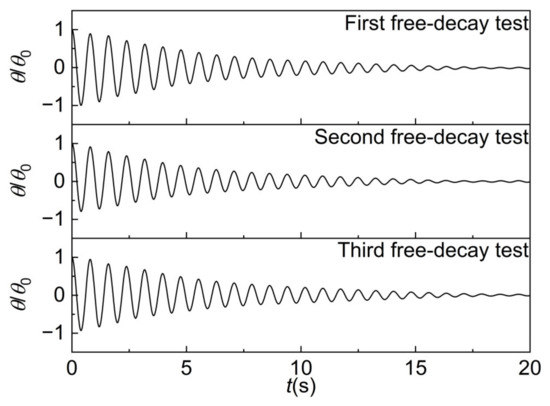
Figure 3.
History of pitch angular displacements of the model in free-decay texts.
3.2. Repeatability and Data Consistency
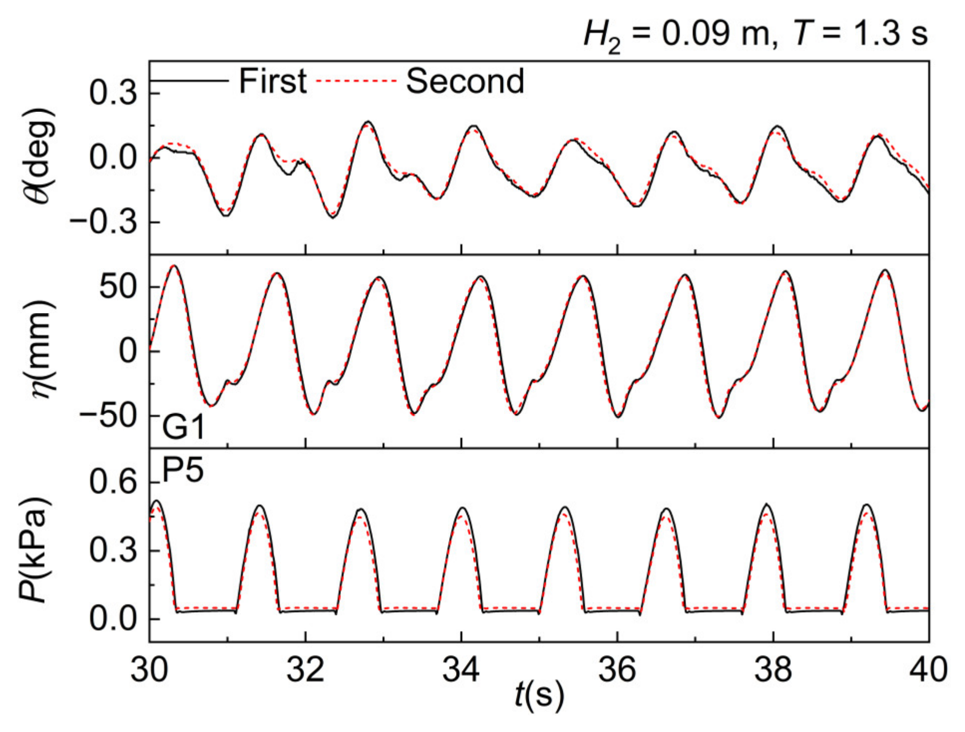
To ensure the accuracy and reliability of the experimental data, repeatability tests were systematically conducted under identical wave conditions. Two independent experimental runs were performed for each test case, with key parameters including angular displacement, wave run-up, and hydrodynamic pressure being measured simultaneously. The results exhibited excellent consistency between repeated trials, as shown in Figure 4. G5 represents the pressure measuring point located 0.48 m from the bottom of the model. The reproducibility verification provides the basis for the subsequent analysis of the results.
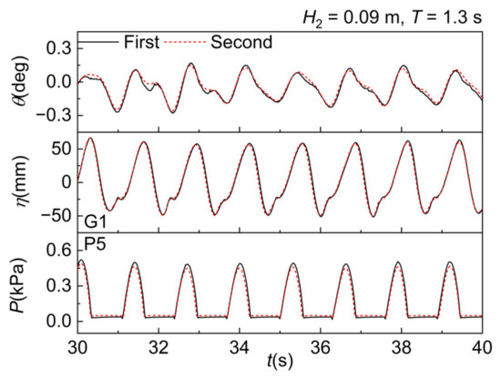
Figure 4.
Reproducibility validation of angular displacement, wave run-up, and hydrodynamic pressure when H2 = 0.09 m and T = 1.3 s.
3.3. Analysis of Nonlinear Vibration Characteristics
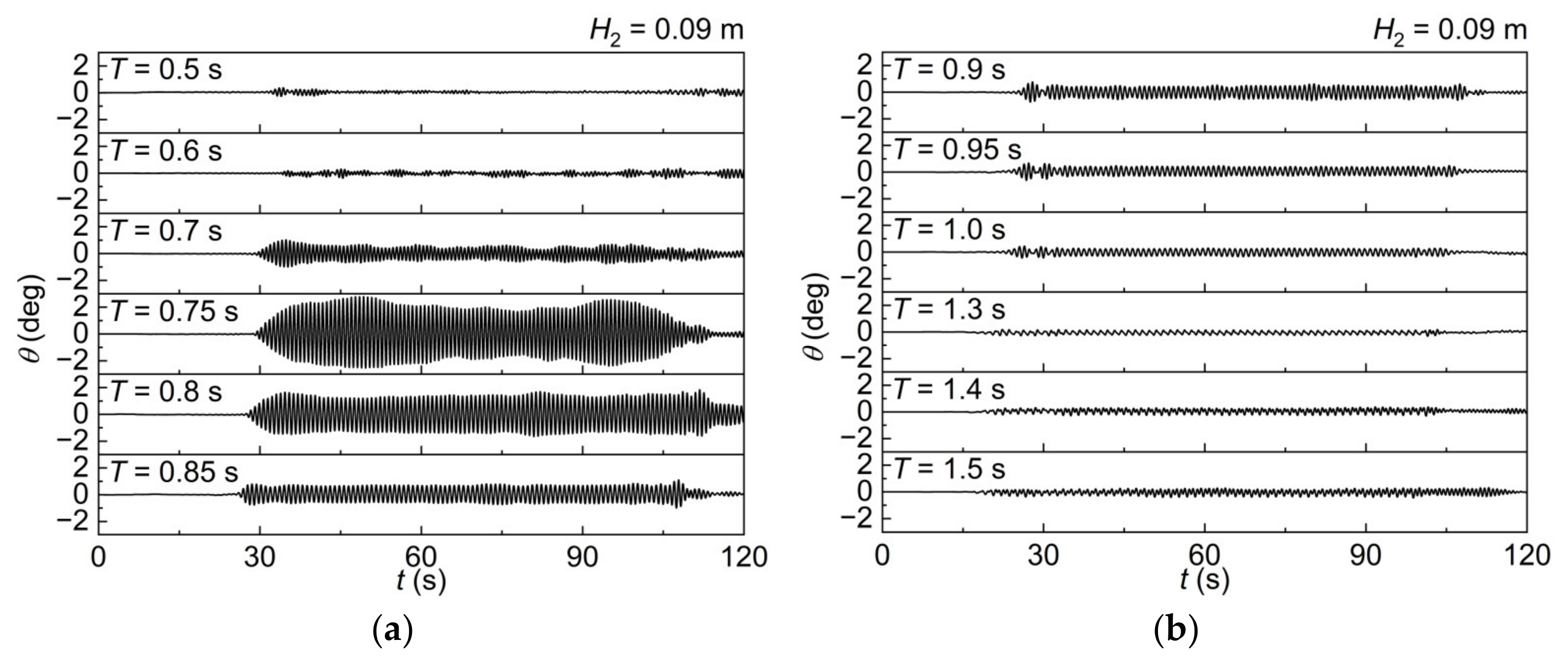
Figure 5 shows the time history of the model’s pitch angular displacements, with wave periods ranging from 0.5 s to 2.9 s and a wave height of H2 = 0.09 m. According to free-decay experiments, the natural period of the model is 0.77 s. It can be observed from Figure 4 that when the wave period is 0.75 s, the model exhibits the most intense vibration, indicating the occurrence of fundamental resonance. This suggests that under this wave period, the incident wave period closely matches the model’s natural frequency, thereby significantly enhancing the transfer of wave energy and amplifying the vibration amplitude. Under other wave period conditions, the vibration amplitude is relatively small. Additionally, in the wave period range of 1.4 s to 1.7 s, the model’s vibration amplitude is noticeably higher than at neighboring periods, with a second harmonic resonance occurring at T = 1.5 s. This indicates that within this period range, the dynamic response of the model is predominantly influenced by nonlinear wave forces, resulting in a significant increase in the vibration amplitude.

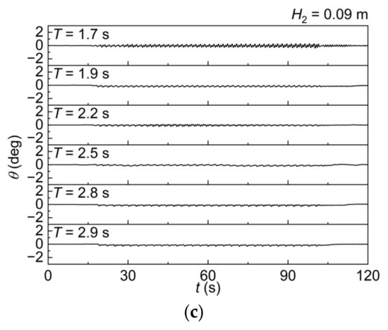
Figure 5.
Time history of pitch angular displacements of model, (a) T = 0.5–0.85 s, (b) T = 0.9–1.5 s, and (c) T = 1.7–2.9 s.
The frequency fast Fourier analysis (FFT) is carried out for the time history of the pitch angular displacements stability section of each period. The wave frequency component and second harmonic component are obtained. The results are presented in Figure 6, illustrating the variation of wave frequency components and second harmonic components with the incident wave period at H2 = 0.09 m. It can be seen from the Figure 6 that the wave frequency component increases with the increase in the wave period in the short period. The peak value of the wave frequency component is reached at T = 0.75 s, and resonance occurs in the model under this experimental condition. With the further increase in wave period, the wave frequency component decreases rapidly. The second harmonic component increases with the increase in the wave period, reaches the peak value of the second harmonic component at the incident wave period T = 1.5 s, and then decreases rapidly. When the incident wave period is close to the natural period of the model, the second harmonic component of the model is approximately equal to 0. When the wave period is close to two times the natural period of the model, the second harmonic component increases significantly. Especially when T = 1.5 s, the second harmonic component reaches the peak value. It distinctly surpasses the wave frequency component, being 2.1 times greater. Under these conditions, the nonlinear effects of the waves have become the primary factor affecting the vibration response of the model.
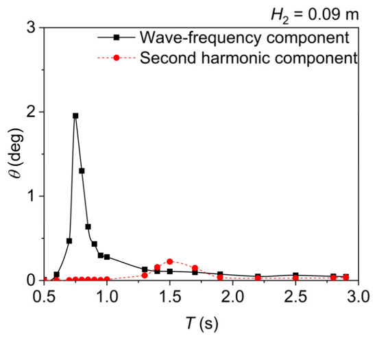
Figure 6.
The wave frequency and second harmonic components of pitch angular displacements of the model, H2 = 0.09 m.
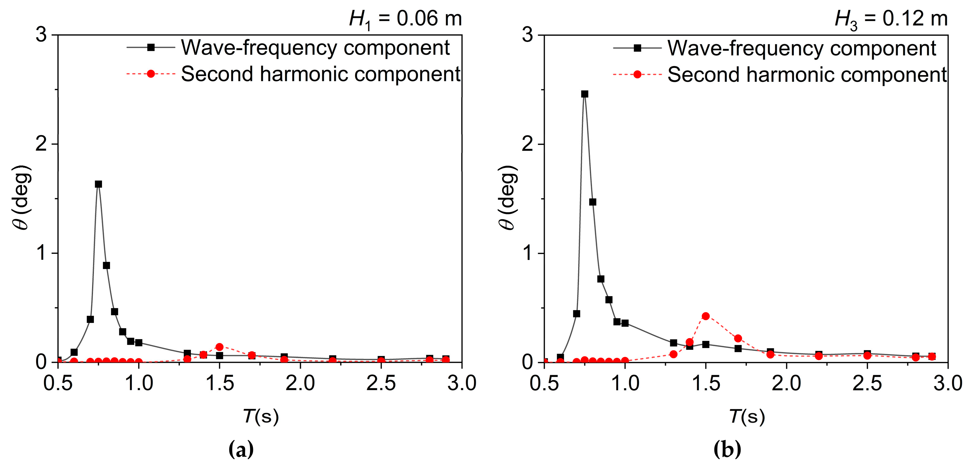
Figure 7 illustrates the variation of both the wave frequency component and the second harmonic component with the incident wave period for H1 = 0.06 m and H3 = 0.12 m. These results are consistent with those obtained for H2 = 0.09 m. The wave frequency component reaches its peak at T = 0.75 s, indicating that the model resonates under these experimental conditions. The second harmonic component increases with the wave period, reaching its maximum at an incident wave period of T = 1.5 s, and then rapidly decreases.
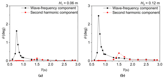
Figure 7.
The wave frequency and second harmonic components of pitch angular displacements of the model, (a) H1 = 0.06 m, (b) H3 = 0.12 m.
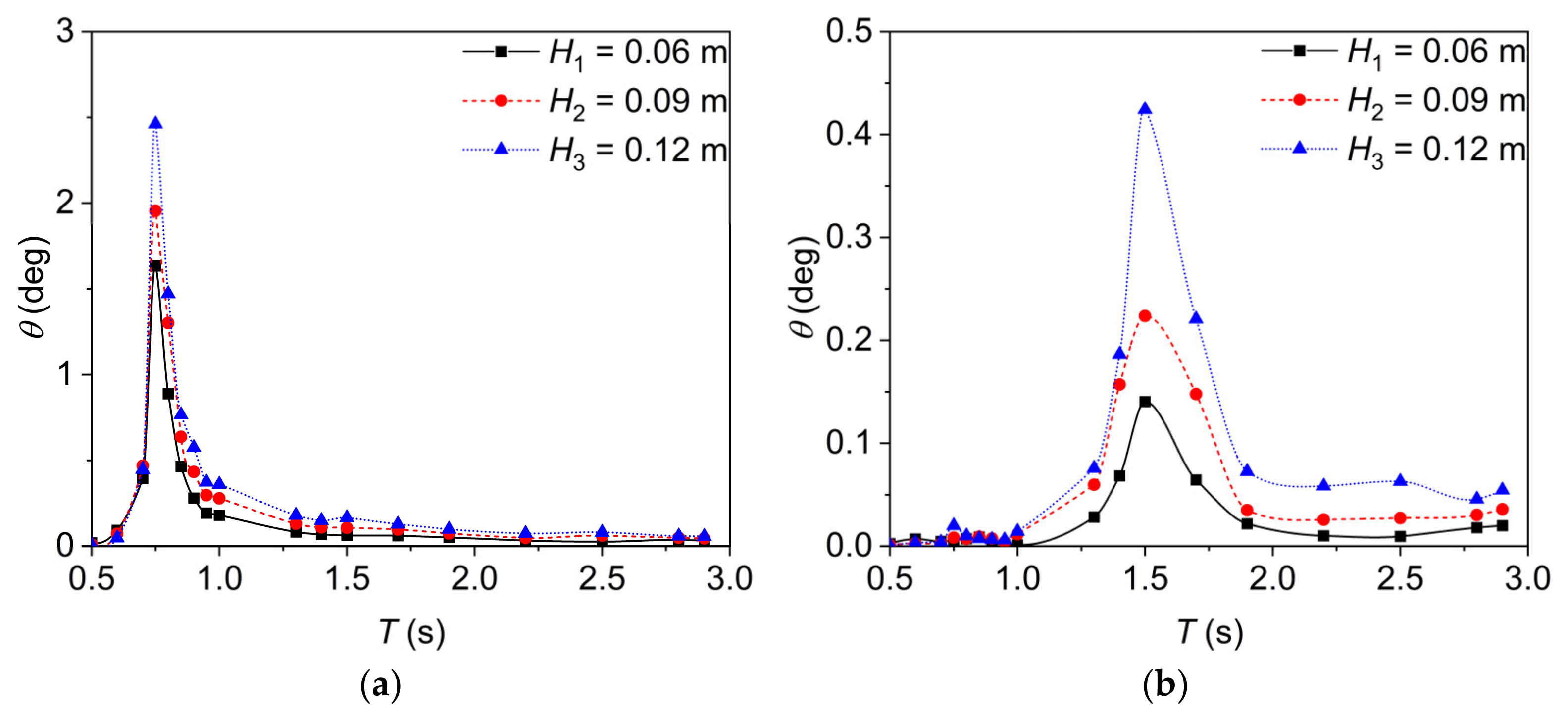
Figure 8 shows the wave frequency component and second harmonic component of pitch angular displacements in the model under different wave heights. The results show that the wave frequency and second harmonic components of the model increase with the increase in wave heights for different incident wave periods. When the incident wave-period is two times the natural period, the nonlinear effect of the wave triggers the second harmonic resonance of the model. The second harmonic component of the model increases significantly. When the wave period is T = 1.5 s, the second harmonic component of a wave height of 0.12 m measures 0.42°, which is three times greater than the second harmonic component of 0.14° associated with a wave height of 0.06 m. It is shown that the second harmonic component of the model does not linearly increase with the increase in wave height. The higher the wave height, the greater the wave steepness, and the stronger the nonlinear effects experienced by the model.

Figure 8.
(a) Wave frequency component and (b) second harmonic component of pitch angular displacements in the model under different wave heights.
3.4. Run-Up on the Model
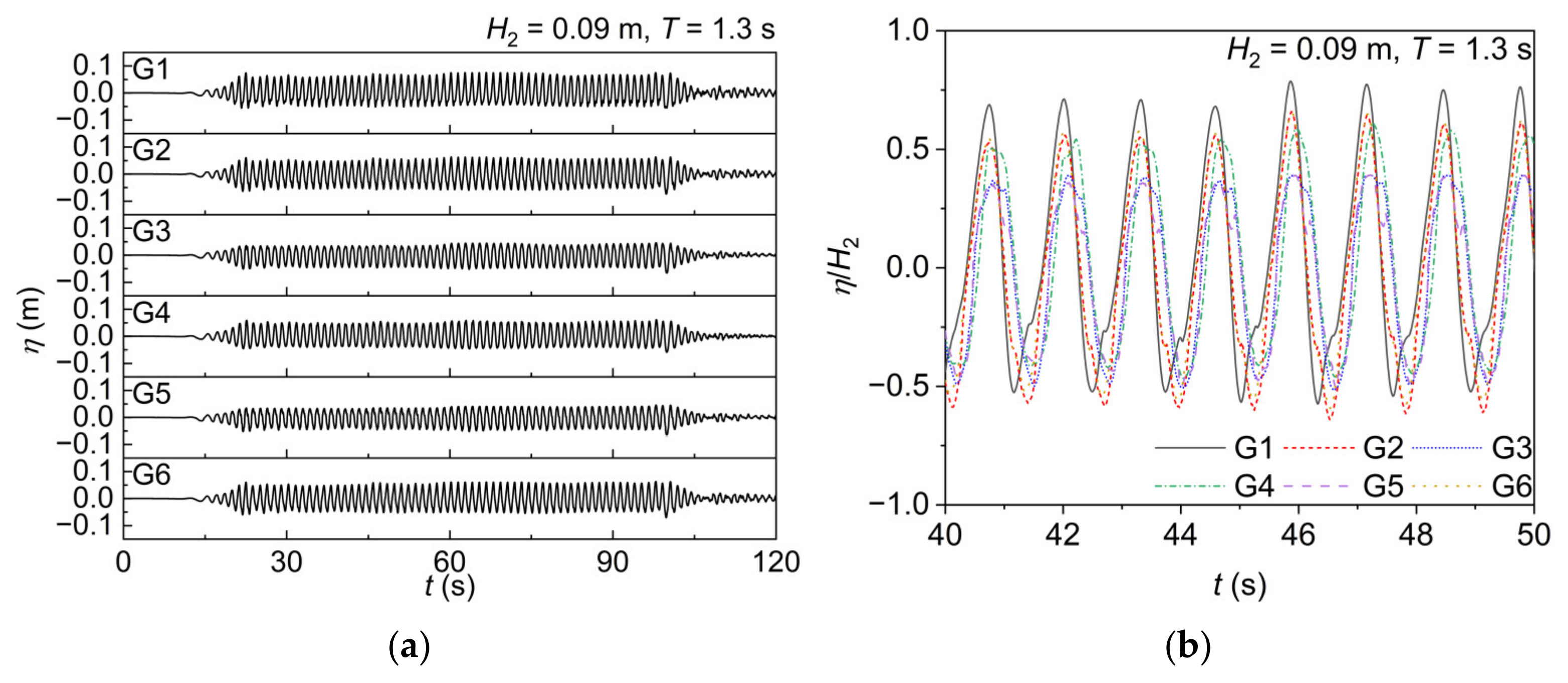
Six wave gauges were uniformly arranged around the model. As shown in Figure 2, the six wave gauges are numbered G1–G6, where G4 records the run-up time history by the model’s back side. When the wave period is T = 1.3 s, it is selected for detailed analysis. At this wave period, the model does not exhibit resonance. In addition, T = 1.3 s lies in the middle range of the wave period for all tests. Figure 9a shows the time history of wave run-up at G1–G6 positions for H2 = 0.09 m and T = 1.3 s. Figure 9b shows the time history of wave height at positions G1–G6 when t = 40–50 s, and the ordinate is the ratio of wave run-up to incident wave height. Figure 8 shows that the run-up of the wave presents sinusoidal characteristics. The run-up of the wave is stable during the whole experiment. The period of vibration is consistent with the period of the incident wave. There is an obvious phase difference between each measuring point. This is caused by the different distance between each measuring point and the wave maker, and the different time required for the wave to propagate to each measuring point.
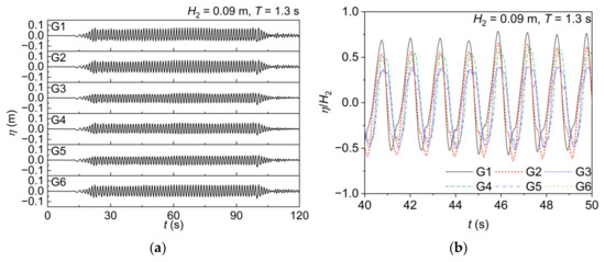
Figure 9.
The wave run-up time history at G1–G6 positions under H2 = 0.09 m and T = 1.3 s for (a) t = 0–120 s and (b) t = 40–50 s.
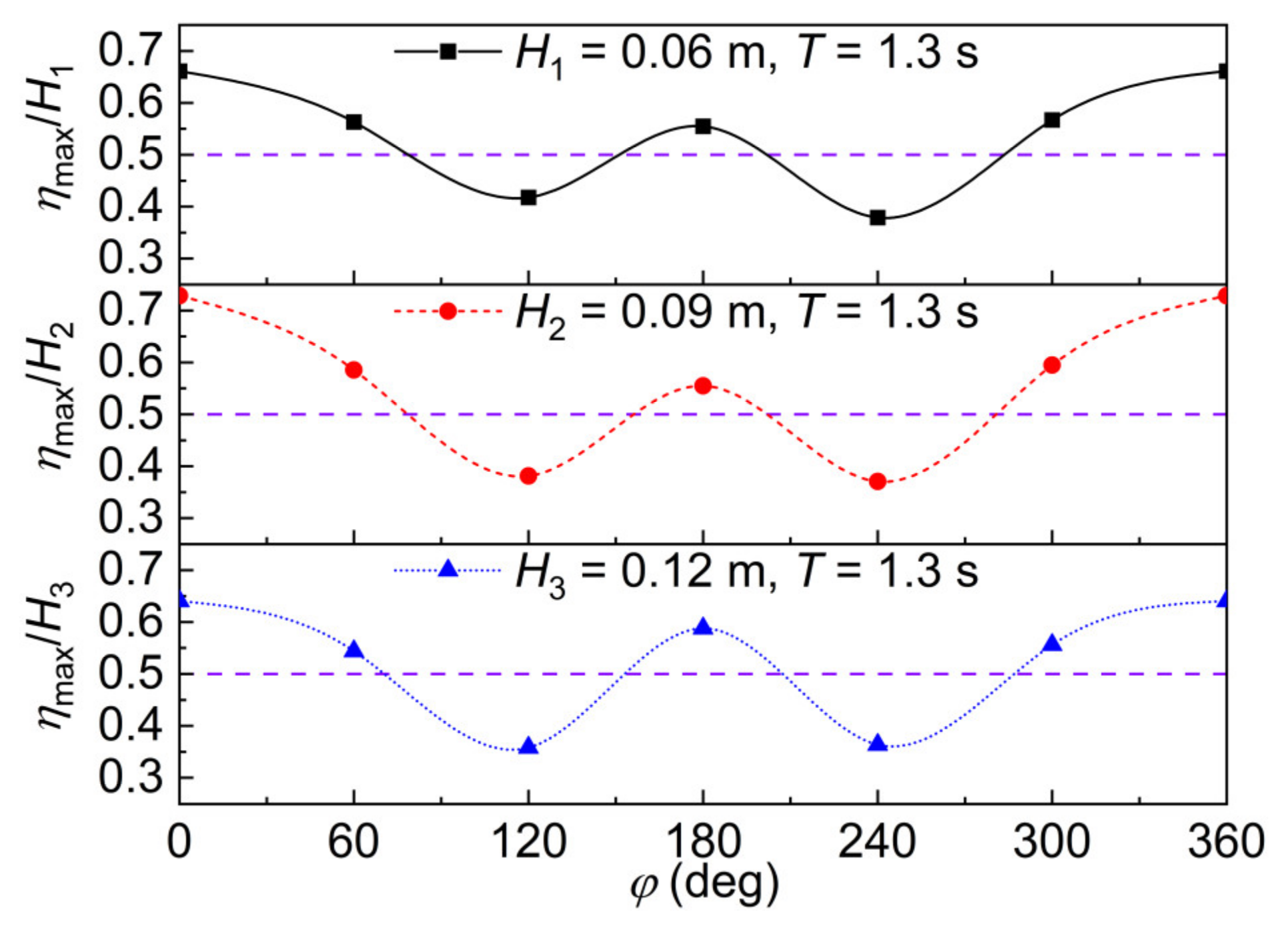
Figure 10 shows the normalized maximum run-up around the model at different wave heights of H1 = 0.06 m, H2 = 0.09 m, and H3 = 0.12 m. The maximum run-up function with respect to φ exhibits a W-shaped distribution. Under all wave conditions, the peak run-up occurs on the incident wave side (φ = 0°), while the minimum values are observed at the lateral positions on the back side (φ = 120° and φ = 240°). Under the condition of H2 = 0.09 m and T = 1.3 s, the highest run-up is observed on the incident wave side, reaching 0.73 times the incident wave height. The wave run-up at the back-side point G4 and at the G2 and G6 positions on both sides of the incident wave side is also greater than half of the incident wave height.
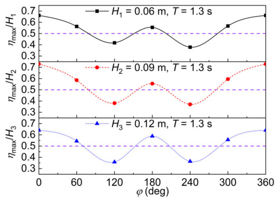
Figure 10.
Normalized maximum run-up around model for wave periods of T = 1.3 s and wave heights of H1 = 0.06 m, H2 = 0.09 m, and H3 = 0.12 m.
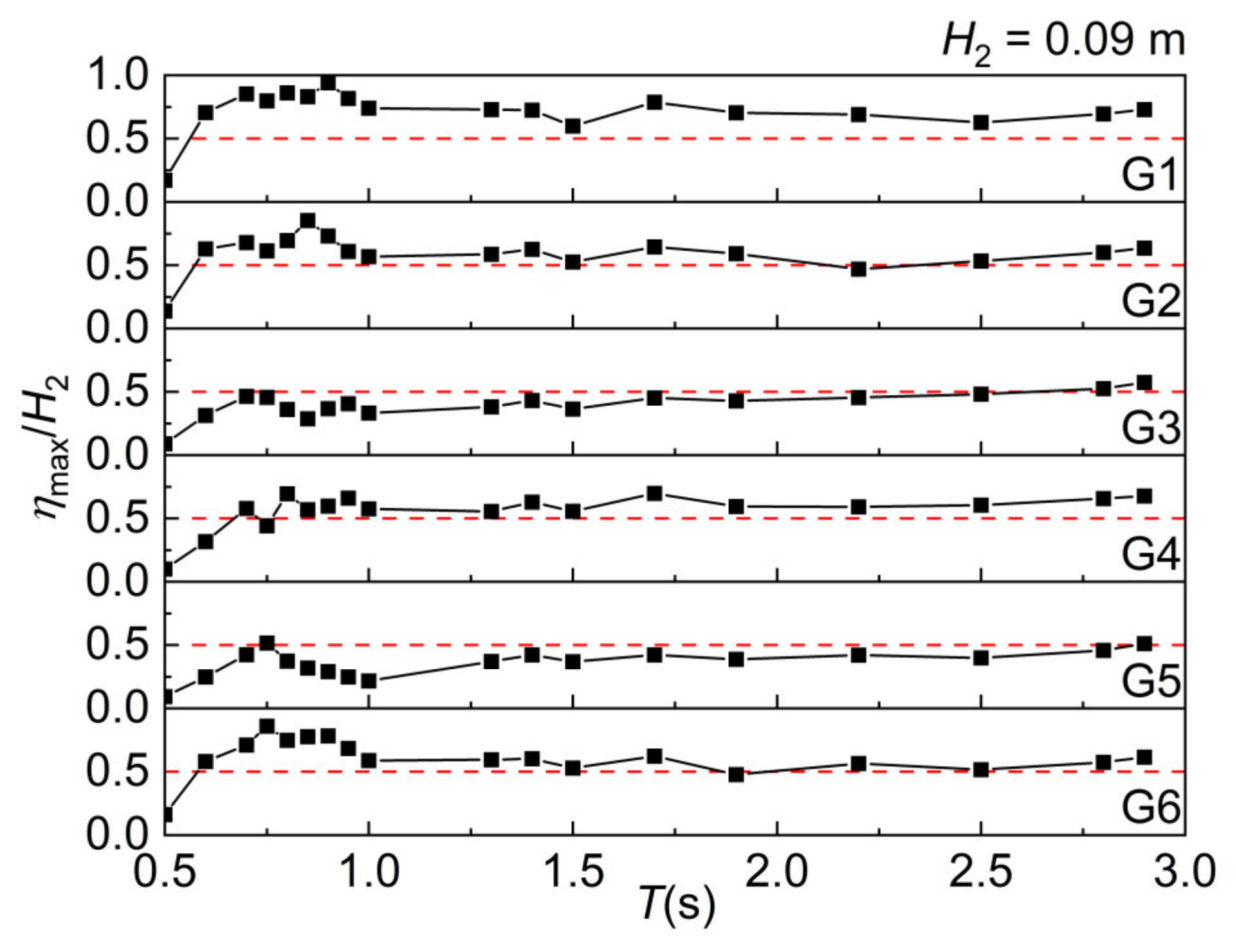
Figure 11 shows the normalized maximum wave run-up for various wave periods under a wave height of H2 = 0.09 m. Except under wave-breaking conditions, the run-up at point G1 consistently exceeds half of the incident wave height. When the wave period is close to the model’s natural period, the run-up increases significantly, with the run-up at point G1 reaching 0.8 times the incident wave height at T = 0.75 s. However, when the model exhibits a second harmonic resonance (T = 1.5 s), the run-up is lower than that observed at neighboring wave periods. In all measured periods, the run-up at points G2, G4, and G6 also exceeds half of the incident wave height, though it remains lower than that at point G1. In most cases, the run-up at the back side, at points G3 and G5, is lower than the amplitude of the incident wave.
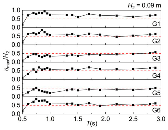
Figure 11.
The normalized maximum wave run-up at different wave periods under the wave height of H2 = 0.09 m.
3.5. Maximum Pressure on the Model
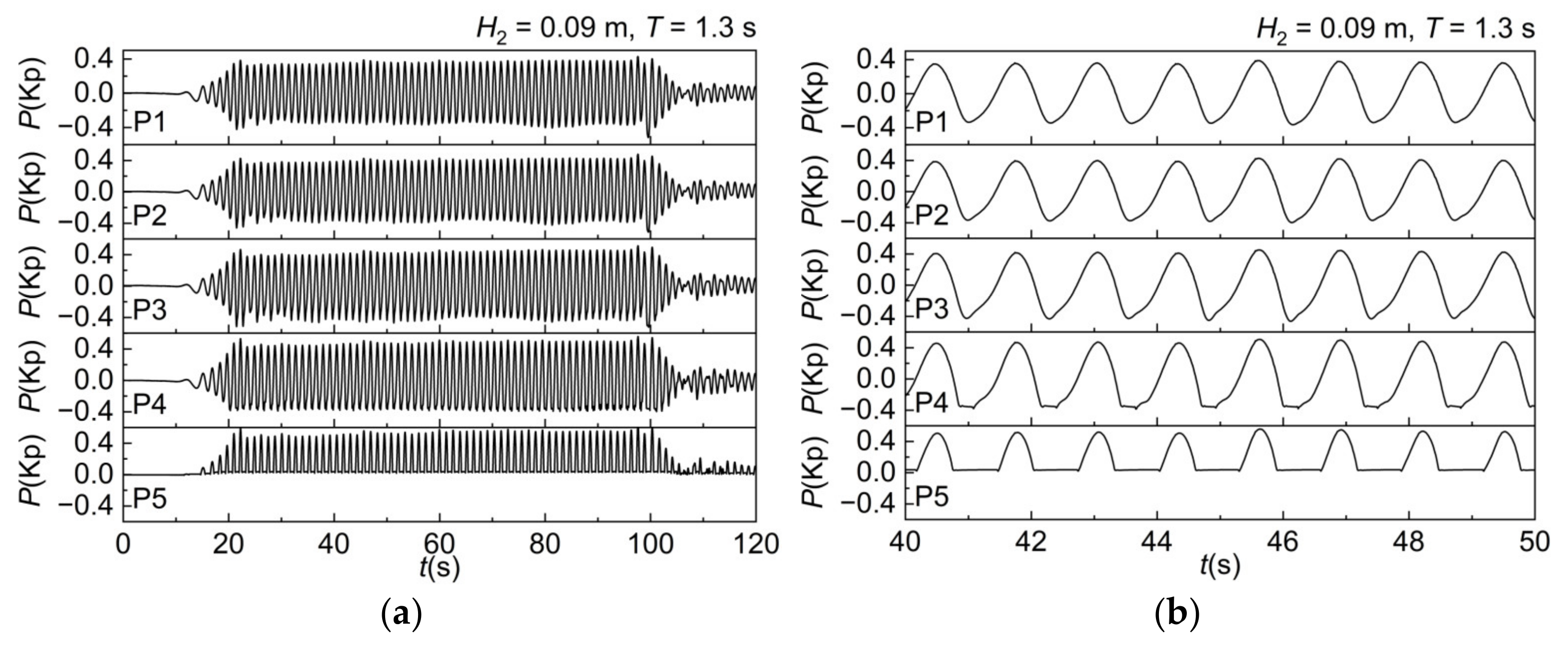
Figure 12a shows the time history of pressure at points P1 to P5 under the wave height of H2 = 0.09 m and the wave period of T = 1.3 s. The vertical heights of the measurement points from the base of the model were set as follows: P1 (0.32 m), P2 (0.36 m), P3 (0.40 m), P4 (0.44 m), and P5 (0.48 m). Figure 12b presents the pressure time history for the time t = 40–50 s. Under the wave action, the pressure experienced on the model fluctuates sinusoidally over time. P1–P4 are located below the water’s surface. During the fluctuations, when the wave reaches its trough, the P4 is already above the water surface. Therefore, the trough of the pressure curve is represented by a straight line, with its value equal to the static water pressure at P4’s initial position. P5 is located at the water’s surface. When this point is at the wave crest, it experiences wave load. When it is at the wave trough, it does not come into contact with the water’s surface. Thus, for half of the period, the pressure value at P5 is zero, as it does not experience wave load during this period.

Figure 12.
The time history of pressure at P1 to P5 for H2 = 0.09 m and T = 1.3 s for (a) t = 0–120 s and (b) t = 40 s–50 s.
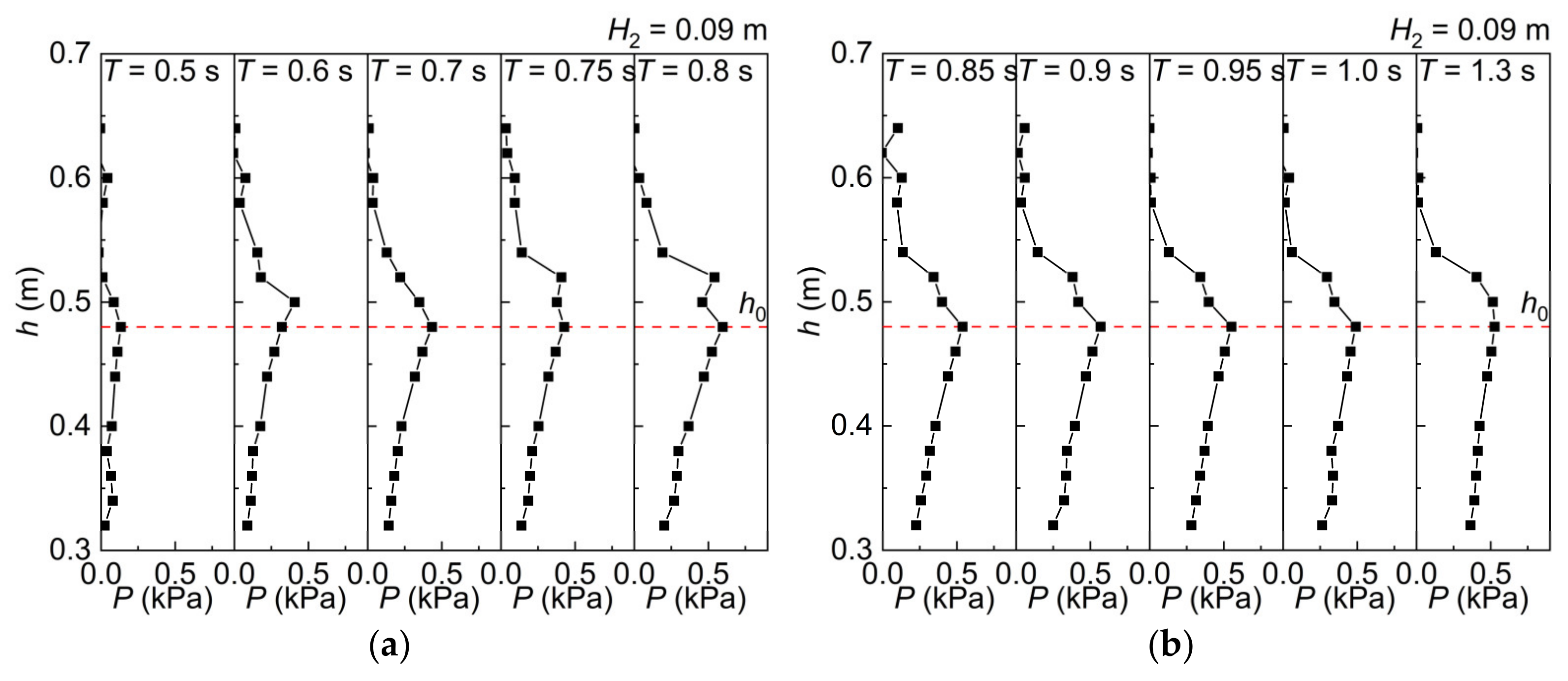
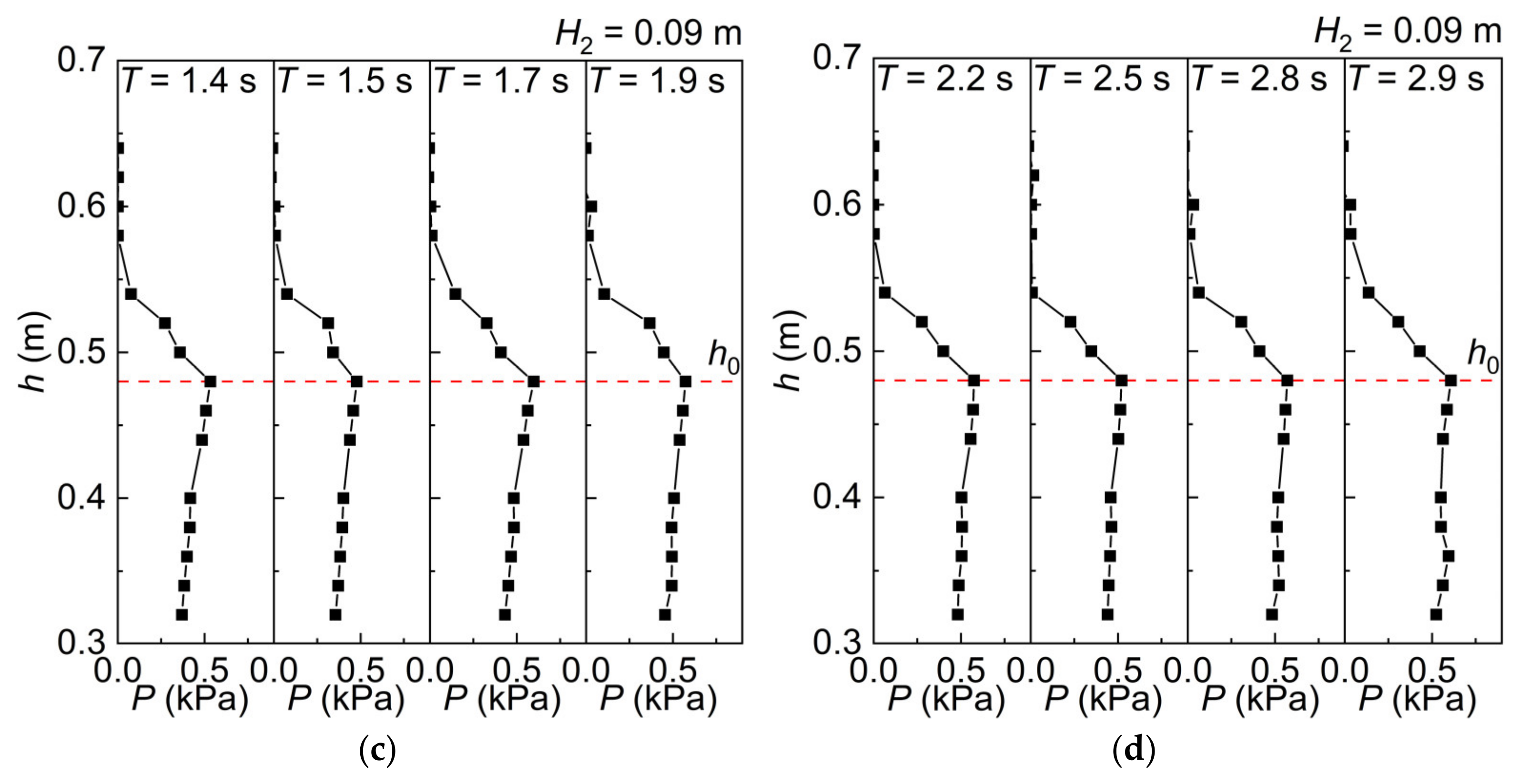
The peak values of pressure were extracted. The vertical axis is the vertical height, and the distribution of maximum pressure with height on the model under different wave period conditions (with the wave height of H2 = 0.09 m) is shown in Figure 13. Here, h0 = 0.48 m is the water depth of the tank. As shown in the Figure 13, the pressure gradually increases from the bottom of the model and reaches its maximum at the water surface. At the water surface, the motion of the water particles is most intense. The relative velocity between the water particles and the model is the highest, resulting in the maximum pressure on the model. Subsequently, as the height increases further, the pressure gradually decreases. When the height reaches a region that is no longer influenced by the fluctuating water surface, the pressure drops to zero. Therefore, the monopile foundation is most affected by wave forces in the area near the water surface. The wave force experienced in regions below the water surface gradually decreases with increasing distance from the water surface.
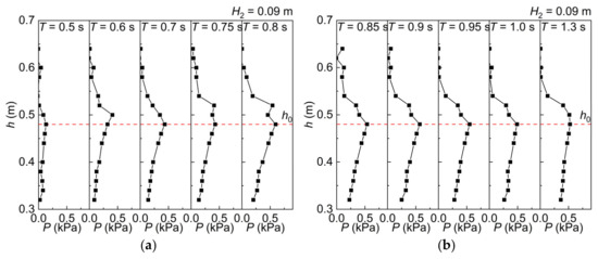
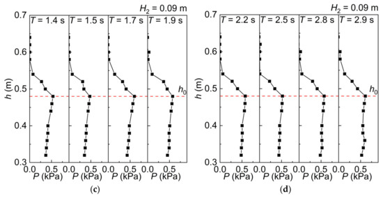
Figure 13.
Maximum pressure with height on the model under different wave period conditions for H2 = 0.09 m: (a) T = 0.5–0.8 s, (b) T = 0.85–1.3 s, (c) T = 1.5–1.9 s, and (d) T = 2.2–21.9 s.
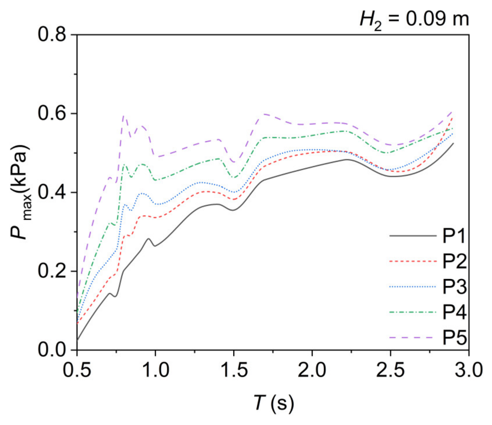
Figure 14 shows the maximum pressure values recorded at P1 to P5 under the wave height of H2 = 0.09 m. The results indicate that, as the wave period increases, the pressure tends to rise. At a period of T = 0.8 s, a peak is observed at positions P3 to P5. However, at a wave period of T = 0.85 s, the pressure drops sharply, falling below the pressure levels at adjacent periods. In addition, at periods of T = 1.0 s, 1.5 s, and 2.5 s, the pressure also exhibits distinct troughs. When the second harmonic resonance occurs in the model, the pressure acting on the model decreases obviously. This phenomenon observed in the experiment becomes increasingly pronounced as the position approaches the water’s surface. At the wave surface, the model exhibits its most significant nonlinear response under the influence of wave action.
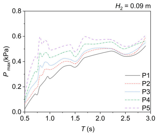
Figure 14.
The maximum pressure values recorded at P1 to P5 for H2 = 0.09 m.
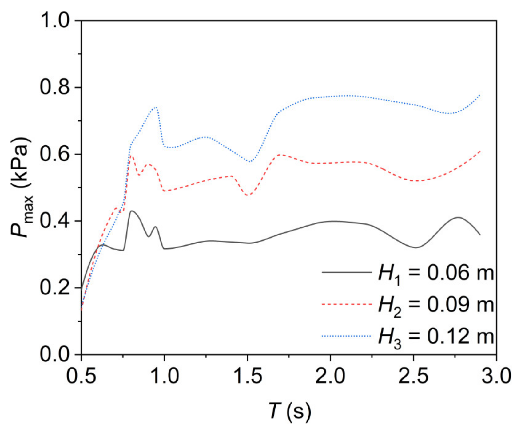
Figure 15 shows the maximum pressure at P5 for various wave periods under wave heights of H1 = 0.06 m, H2 = 0.09 m, and H3 = 0.12 m. Under high frequency wave conditions (for example, at T = 0.5 s for H1 = 0.06 m; at T = 0.5 s, 0.6 s, and 0.7 s for H2 = 0.09 m; and at T = 0.5 s, 0.6 s, 0.7 s, and 0.75 s for H3 = 0.12 m), the incident waves break, resulting in rather erratic pressure data. The measured pressure values are relatively lower compared to other test conditions. This clearly demonstrates that the incident wave height has a significant effect on the pressure experienced by the model. As the wave height increases, the pressure at P5 in each period also increases. Furthermore, the second harmonic resonance phenomena of the model caused by the nonlinear effects of the waves affect the pressure at each position. Under wave conditions with T = 1.5 s, the pressure at P5 is smaller than that experienced by the model during the surrounding wave period. This phenomenon becomes more obvious with the increase in incident wave height.
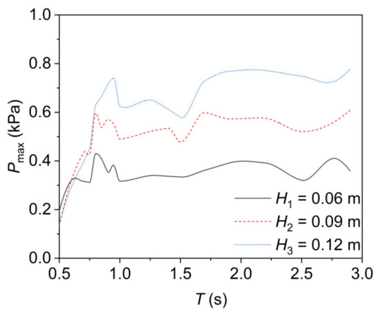
Figure 15.
The maximum pressure at P5 for H1 = 0.06 m, H2 = 0.09 m, and H3 = 0.12 m, respectively.
4. Conclusions
A physical model experiment was carried out in a wave tank. The nonlinear vibration response of a flexible monopile-foundation offshore wind turbine model under regular wave action was studied. The wave run-up around the model and the maximum pressure on the model were also analyzed. The experiment covered many conditions, such as wave height and wave period, and the main conclusions are as follows:
The change of wave period has significant influence on the vibration response of the model at different wave heights. When the wave period is the natural period of the model, a resonance phenomenon appears in the model. The model exhibits large vibration amplitudes. When the wave period approaches two times the natural period of the model, the model vibration response is markedly enhanced. In these conditions, the nonlinear effects of the waves trigger a second harmonic resonance of the model, resulting in a significant increase in the amplitude of the second harmonic component. The second harmonic component of the model does not linearly increase with the increase in wave height. The higher the wave height, the stronger the nonlinear effects experienced by the model.
The maximum run-up around the model is W-shaped in the circumferential direction. The peak run-up occurs on the incident wave side (φ = 0°), while the minimum values are observed at the lateral positions on the back side (φ = 120° and φ = 240°). The wave run-up at back-side point G4 and at the G2 and G6 positions on both sides of the incident wave side is also greater than half of the incident wave height. When the model undergoes a second harmonic resonance, the wave run-up is lower than the wave run-up of other wave periods.
The pressure gradually increases from the bottom of the model and reaches its maximum at the water surface. Above the water surface, the pressure decreases as the height increases. With the increase in wave height, the pressure at each position and wave period also increases. When the model has secondary resonance, the pressure acting on the model is obviously reduced. This phenomenon is most obvious at the wave surface.
This study primarily investigates the phenomenon of a second harmonic resonance in a monopile offshore wind turbine model subjected to regular wave conditions. Utilizing the principles of Froude similarity, the experimental model is designed to reflect, to some extent, the dynamic response characteristics of an actual turbine foundation. However, due to certain simplifications in the current model design, its responses do not fully encapsulate those of the real system. Consequently, future research will concentrate on further optimizing the model design to more accurately simulate the behavior of a turbine foundation within an oceanic environment.
Author Contributions
Conceptualization, S.W.; methodology, S.W. and X.L.; formal analysis, S.W.; investigation, S.W., H.Z. and Z.C.; resources, S.W. and L.Z.; data curation, S.W. and H.Z.; writing—original draft preparation, S.W. and H.Z.; writing—review and editing, S.W., H.Z., Z.C., X.L., L.Z., M.D., R.L. and D.L.; visualization, S.W., H.Z. and Z.C.; supervision, S.W; project administration, S.W.; funding acquisition, S.W. All authors have read and agreed to the published version of the manuscript.
Funding
This work is supported by the National Key R&D Program of China (2022YFB4201400) and China Three Gorges Corporation (NBZZ202400326).
Data Availability Statement
The data that support the findings of this study are available from the corresponding author upon reasonable request.
Conflicts of Interest
Authors Songxiong Wu, Hao Zhang, Ziwen Chen, Xiaoting Liu, Long Zheng, Mengjiao Du and Donghai Li were employed by the company China Three Gorges Corporation. Author Rongfu Li was employed by the company Goldwind Sci & Tech Co., Ltd. The remaining authors declare that the research was conducted in the absence of any commercial or financial relationships that could be construed as a potential conflict of interest.
References
- Sun, X.; Huang, D.; Wu, G. The Current State of Offshore Wind Energy Technology Development. Energy 2012, 41, 298–312. [Google Scholar] [CrossRef]
- Arshad, M.; O’Kelly, B.C. Analysis and Design of Monopile Foundations for Offshore Wind-Turbine Structures. Mar. Georesources Geotechnol. 2016, 34, 503–525. [Google Scholar] [CrossRef]
- Bošnjaković, M.; Katinić, M.; Santa, R.; Marić, D. Wind Turbine Technology Trends. Appl. Sci. 2022, 12, 8653. [Google Scholar] [CrossRef]
- Wu, X.; Hu, Y.; Li, Y.; Yang, J.; Duan, L.; Wang, T.; Adcock, T.; Jiang, Z.; Gao, Z.; Lin, Z.; et al. Foundations of Offshore Wind Turbines: A Review. Renew. Sustain. Energy Rev. 2019, 104, 379–393. [Google Scholar] [CrossRef]
- Schløer, S.; Bredmose, H.; Bingham, H.B. The Influence of Fully Nonlinear Wave Forces on Aero-Hydro-Elastic Calculations of Monopile Wind Turbines. Mar. Struct. 2016, 50, 162–188. [Google Scholar] [CrossRef]
- Chou, J.-S.; Tu, W.-T. Failure Analysis and Risk Management of a Collapsed Large Wind Turbine Tower. Eng. Fail. Anal. 2011, 18, 295–313. [Google Scholar] [CrossRef]
- Chen, X.; Xu, J.Z. Structural Failure Analysis of Wind Turbines Impacted by Super Typhoon Usagi. Eng. Fail. Anal. 2016, 60, 391–404. [Google Scholar] [CrossRef]
- Morris-Thomas, M.T.; Thiagarajan, K.P. The Run-up on a Cylinder in Progressive Surface Gravity Waves: Harmonic Components. Appl. Ocean Res. 2004, 26, 98–113. [Google Scholar] [CrossRef]
- Niedzwecki, J.M.; Duggal, A.S. Wave Runup and Forces on Cylinders in Regular and Random Waves. J. Waterw. Port Coast. Ocean Eng. 1992, 118, 615–634. [Google Scholar] [CrossRef]
- Marino, E.; Lugni, C.; Borri, C. A Novel Numerical Strategy for the Simulation of Irregular Nonlinear Waves and Their Effects on the Dynamic Response of Offshore Wind Turbines. Comput. Methods Appl. Mech. Eng. 2013, 255, 275–288. [Google Scholar] [CrossRef]
- Marino, E.; Lugni, C.; Borri, C. The Role of the Nonlinear Wave Kinematics on the Global Responses of an OWT in Parked and Operating Conditions. J. Wind Eng. Ind. Aerodyn. 2013, 123, 363–376. [Google Scholar] [CrossRef]
- Paulsen, B.T.; Bredmose, H.; Bingham, H.B.; Schløer, S. Steep Wave Loads From Irregular Waves on an Offshore Wind Turbine Foundation: Computation and Experiment. In Proceedings of the ASME 2013 32nd International Conference on Ocean, Offshore and Arctic Engineering, Nantes, France, 9–14 June 2013; American Society of Mechanical Engineers: New York, NY, USA, 2013; Volume 9, p. V009T12A028. [Google Scholar]
- Deng, S.; Qin, M.; Ning, D.; Lin, L.; Wu, S.; Zhang, C. Numerical and Experimental Investigations on Non-Linear Wave Action on Offshore Wind Turbine Monopile Foundation. J. Mar. Sci. Eng. 2023, 11, 883. [Google Scholar] [CrossRef]
- Bredmose, H.; Jacobsen, N.G. Breaking Wave Impacts on Offshore Wind Turbine Foundations: Focused Wave Groups and CFD. In Proceedings of the 29th International Conference on Ocean, Offshore and Arctic Engineering, Shanghai, China, 6–11 June 2010; ASMEDC: New York, NY, USA, 2010; Volume 3, pp. 397–404. [Google Scholar]
- Ding, H.; Zhao, G.; Tang, T.; Taylor, P.H.; Adcock, T.A.; Dai, S.; Ning, D.; Chen, L.; Li, J.; Wang, R.; et al. Experimental investigation of nonlinear forces on a monopile offshore wind turbine foundation under directionally spread waves. J. Offshore Mech. Arct. Eng. 2025, 147, 042002. [Google Scholar] [CrossRef]
- Sclavounos, P.D.; Zhang, Y.; Ma, Y.; Larson, D.F. Offshore Wind Turbine Nonlinear Wave Loads and Their Statistics. J. Offshore Mech. Arct. Eng. 2019, 141, 031904. [Google Scholar] [CrossRef]
- Mockutė, A.; Marino, E.; Lugni, C.; Borri, C. Comparison of Nonlinear Wave-Loading Models on Rigid Cylinders in Regular Waves. Energies 2019, 12, 4022. [Google Scholar] [CrossRef]
- De Ridder, E.J.; Aalberts, P.; Van Den Berg, J.; Buchner, B.; Peeringa, J. The Dynamic Response of an Offshore Wind Turbine With Realistic Flexibility to Breaking Wave Impact. In Proceedings of the ASME 2011 30th International Conference on Ocean, Offshore and Arctic Engineering, Rotterdam, The Netherlands, 19–24 June 2011; ASMEDC: New York, NY, USA, 2011; Volume 5, pp. 543–552. [Google Scholar]
- Bachynski, E.E.; Ormberg, H. Hydrodynamic Modeling of Large-Diameter Bottom-Fixed Offshore Wind Turbines. In Proceedings of the ASME 2015 34th International Conference on Ocean, Offshore and Arctic Engineering, St. John’s, NL, Canada, 31 May–5 June 2015; American Society of Mechanical Engineers: New York, NY, USA, 2015; Volume 9, p. V009T09A051. [Google Scholar]
- Ryan, G.V.; Tang, T.; McAdam, R.A.; Adcock, T.A. Influence of non-linear wave load models on monopile supported offshore wind turbines for extreme conditions. Ocean Eng. 2025, 323, 120510. [Google Scholar] [CrossRef]
- Jiang, C.; el Moctar, O. Experimental decomposition of nonlinear hydrodynamic loads and hydroelastic responses in wave–structure interactions of monopile wind turbines. Phys. Fluids 2024, 36, 117112. [Google Scholar] [CrossRef]
- Wang, S.; Larsen, T.J.; Bredmose, H. Ultimate load analysis of a 10 MW offshore monopile wind turbine incorporating fully nonlinear irregular wave kinematics. Mar. Struct. 2021, 76, 102922. [Google Scholar] [CrossRef]
- Bachynski, E.; Thys, M.; Delhaye, V. Dynamic Response of a Monopile Wind Turbine in Waves: Experimental Uncertainty Analysis for Validation of Numerical Tools. Appl. Ocean Res. 2019, 89, 96–114. [Google Scholar] [CrossRef]
- Bachynski, E.E.; Thys, M.; Dadmarzi, F.H. Observations from Hydrodynamic Testing of a Flexible, Large-Diameter Monopile in Irregular Waves. J. Phys. Conf. Ser. 2020, 1669, 012028. [Google Scholar] [CrossRef]
- Suja-Thauvin, L.; Krokstad, J.R.; Bachynski, E.E.; De Ridder, E.-J. Experimental Results of a Multimode Monopile Offshore Wind Turbine Support Structure Subjected to Steep and Breaking Irregular Waves. Ocean Eng. 2017, 146, 339–351. [Google Scholar] [CrossRef]
- Bredmose, H.; Dixen, M.; Ghadirian, A.; Larsen, T.J.; Schløer, S.; Andersen, S.J.; Wang, S.; Bingham, H.B.; Lindberg, O.; Christensen, E.D.; et al. DeRisk—Accurate Prediction of ULS Wave Loads. Outlook and First Results. Energy Procedia 2016, 94, 379–387. [Google Scholar] [CrossRef]
- Nielsen, A.W.; Schlütter, F.; Sørensen, J.V.T.; Bredmose, H. Wave Loads on a Monopile in 3D Waves. In Proceedings of the ASME 2012 31st International Conference on Ocean, Offshore and Arctic Engineering, Rio de Janeiro, Brazil, 1–6 June 2012; American Society of Mechanical Engineers: New York, NY, USA, 2012; Volume 7, pp. 403–411. [Google Scholar]
- Paulsen, B.T.; Bredmose, H.; Bingham, H.B. An Efficient Domain Decomposition Strategy for Wave Loads on Surface Piercing Circular Cylinders. Coast. Eng. 2014, 86, 57–76. [Google Scholar] [CrossRef]
- Bredmose, H.; Slabiak, P.; Sahlberg-Nielsen, L.; Schlütter, F. Dynamic Excitation of Monopiles by Steep and Breaking Waves: Experimental and Numerical Study. In Proceedings of the ASME 2013 32nd International Conference on Ocean, Offshore and Arctic Engineering, Nantes, France, 9–14 June 2013; American Society of Mechanical Engineers: New York, NY, USA, 2013; Volume 8, p. V008T09A062. [Google Scholar]
- Suja-Thauvin, L.; Krokstad, J.R.; Bachynski, E.E. Critical Assessment of Non-Linear Hydrodynamic Load Models for a Fully Flexible Monopile Offshore Wind Turbine. Ocean Eng. 2018, 164, 87–104. [Google Scholar] [CrossRef]
- Bachynski, E.E.; Kristiansen, T.; Thys, M. Experimental and Numerical Investigations of Monopile Ringing in Irregular Finite-Depth Water Waves. Appl. Ocean Res. 2017, 68, 154–170. [Google Scholar] [CrossRef]


Disclaimer/Publisher’s Note: The statements, opinions and data contained in all publications are solely those of the individual author(s) and contributor(s) and not of MDPI and/or the editor(s). MDPI and/or the editor(s) disclaim responsibility for any injury to people or property resulting from any ideas, methods, instructions or products referred to in the content. |
© 2025 by the authors. Licensee MDPI, Basel, Switzerland. This article is an open access article distributed under the terms and conditions of the Creative Commons Attribution (CC BY) license (https://creativecommons.org/licenses/by/4.0/).