Field Calibration of a Time-Domain Reflectometry Sensor for Water Content Measurement in Soils with Low Content of Coarse Fragments ^†

Abstract

Comparison of soil water sensors for irrigation scheduling requires an accurate reference measurement. An Acclima TDR-310H soil water content sensor was calibrated and validated for sand, loamy sand, clay loam, sandy clay loam, and sandy loam soils. In 2021, sensor readings and soil samples were collected in the same sensor volume at depths of 15 and 46 cm at three irrigated field sites with five stations each. Gravimetric water content, bulk density, and volumetric water content (θ_v) were determined in the lab. The root mean square error was 0.032 cm³ cm⁻³, which was within acceptable limits. The sensor underestimated θ_v with a mean bias error of −0.025 cm³ cm⁻³. The linear field calibration equation was θ_v-Sample = 0.9498 θ_v-TDR + 0.0357 with R² = 0.8984. t-tests showed that the 95% confidence intervals (CIs) were 0.82 < slope < 1.08 and 0.0072 < intercept < 0.0642. Since the field calibration result was different from the factory calibration (intercept CI not straddling 0), use of the field calibration is recommended. A validation dataset collected in 2023 confirmed the calibration equation. The calibrated sensor can be used to evaluate other θ_v sensors for irrigation scheduling in the soil types in this study.

1. Introduction

About 70% of the use of the world’s freshwater resources is for irrigation purposes [1]. Therefore, irrigation water should be used judiciously, but improper management of irrigation water can both cause loss of water and degrade crop and environment quality. According to [2], irrigation water loss can be reduced by using efficient agricultural technologies, applying proper irrigation scheduling, and implementing deficit irrigation. Among these categories, improvement of irrigation scheduling has the largest potential for water savings [3]. One of the most popular techniques of irrigation scheduling is the measurement of soil water content and applying water according to the plants’ need. Advanced irrigation technologies such as in situ sensors can be used in this case for soil water content monitoring.

Numerous techniques and instruments have been proposed or developed to estimate soil water content, such as gravimetric, tensiometers, gypsum blocks, granular matrix sensors, neutron probes, time-domain reflectometry (TDR), and capacitance probes. Electromagnetic sensors such as TDR can be used to continuously monitor soil water content. A TDR sensor sends an electromagnetic wave along two wave guides which have been inserted in the soil; a fast oscilloscope is used to capture the wave after it is reflected back. The waveform is then used to determine the travel time which provides a direct measurement of the soil’s apparent permittivity. The permittivity of water is much higher than the permittivity of air or the solid phase of soil; therefore, apparent dielectric permittivity of the soil is highly correlated to the volumetric water content (θ_v, cm³ cm⁻³) [3]. The Acclima TDR uses the Topp equation [4] to determine θ_v. The Acclima TDR-310H (Acclima, Inc., Meridian, ID, USA) was chosen for this study because it can be installed vertically with little or no soil or crop disturbance compared to Acclima’s model TDR-315. Especially considering installation depths greater than 15 cm, the Acclima TDR-310H sensor has a round shape that can be attached to an extension pipe and installed in a narrow, vertical hole. Acclima TDR-305 also has a round shape with a smaller sampling volume than Acclima TDR-310H, while the 305 can handle higher soil salinity values at the expense of a smaller sampling volume. Since the 310 range for salinity was acceptable for our study, its larger sensing volume was better for our study. Furthermore, our prior experience testing of the Acclima sensors supported our selection of the Acclima TDR-310H for this study. However, even TDR readings can be affected by factors such as soil texture and structure, bulk electrical conductivity, crop type, root development, etc., which can reduce the effectiveness of sensor measurement [5,6]. As a result, it is helpful to calibrate TDR sensors with in situ undisturbed soils [7]. In this context, “undisturbed” refers to soils in place in production settings rather than never-tilled soils.

The performance of a factory calibrated Acclima TDR-315 sensor was assessed by [8] in low and high saline soil, who found that it showed overestimation when measuring soil moisture thresholds, specifically field capacity and permanent wilting point. Also, the TDR sensor did not perform well in a high-saline soil. Ref. [9] calibrated a TDR sensor in the lab with three different soil types (silty clay loam, clay, and clay loam) and observed that higher bulk electrical conductivity (BEC) values for silty clay loam and clay soils correspond to larger slopes. The higher BEC was the result of higher clay content. Ref. [10] calibrated a TDR sensor both in the field and the lab and identified a difference in calibration results from the manufacturer. Therefore, the author suggested conducting a soil-specific calibration to improve the sensor accuracy.

Table 1. List of published papers focusing specifically on calibration of TDR soil water sensor.

Reference	Lab/Field	Soil Type	Setting or Purpose	Sensor Type	Site(s)	Statistics a	Soil Water Content Release Curve b	Brief Summary
[11]	Field	Sandy loam	Irrigation	TDR, Aquaflex	1	R2	No	TDR sensor was calibrated using the gravimetric method, and the obtained R2 was 0.98
[8]	Factory calibration	Sandy loam, silty clay loam	Irrigation	TDR315, CS655, GSI, SM100, CropX	2	RMSE, RSR, MBE, index of agreement (k), Pearson correlation coefficient (r)	No	TDR sensor overestimated in fine sandy loam and silty clay loam soil with RMSE values of 0.028 and 0.064 m3 m−3, respectively
[9]	Lab	Silty clay, clay, clay loam	Irrigation	TDR-100		Slope, intercept, R2, RMSE	No	Sensor underestimated in each of the soil types when the soil was air dried (RMSE 0.0196, 0.0085, and 0.0097 m3 m−3, respectively) and overestimated when silty clay and clay soil was saturated (RMSE 0.00364, 0.00353, and 0.00189 m3 m−3, respectively)
[7]	Field and Lab	Six soil types	Irrigation	TDR315, CS655, GSI	2	R2, RMSE	No	TDR315 overestimated θv for clay soil, with an RMSE range from 0.03 to 0.17 cm3 cm−3
[12]	Lab	Sandy, sandy–feldspathic sandstone mixture (3:1), loessial, dark loessial, and Lou soil	Hydrological application	TDR315L, Diviner 2000	6	R2, RMSE	No	An average R2 of 0.9820 and RMSE of 0.026 m3 m−3 was obtained by the TDR315L sensor
[13]	Lab	28 soil types	Irrigation	TDR	14	R2	No	Clay and fine particles affected the sensor EC readings with the lowest R2 of 0.3861
[14]	Field	Silt loam, loamy sand	Irrigation	TDR315L, CS616, CS655, 5TE, 10HS, EC-5, SM150, JD field connect, TEROS 21(MPS-6)	2	RMSE, MBE, R2, SE, CI	Yes	Acclima TDR351L sensor performed better in the loamy sand soil, with an RMSE of 0.02 m3 m−3
[10]	Field and Lab	Eolian sand, clay	Irrigation	TDR	1	t-test	No	Sensor responded well with continuous drip irrigation
[15]	Lab	Saline soil	Strength and stability of soil structure	TDR	1	R2, absolute error	No	TDR overestimated moisture content, with an R2 of 0.8464
[16]	Lab	Silt loam and loamy sand	Irrigation	TDR300 (High clay mode), TDR300 (Standard mode), 5TE, 10HS, SM150, CS616, CS620	2	RMSE	No	TDR300 high clay mode sensor performed best in the silt loam soil, with an RMSE of 0.020 m3 m−3
(This study)	Field	Sand, loamy sand, clay loam, sandy clay loam, and sandy loam	Irrigation	TDR-310H	3	RMSE, MBE, slope, intercept, R2, t-test, CI	No	TDR-310H underestimated θv, with an RMSE of 0.032 cm3 cm−3, an MBE of −0.025 cm3 cm−3, and an R2 of 0.8984

^a Abbreviations: MBE = mean bias error; RMSE = root mean square error; R² = coefficient of determination; SE = standard error; CI = confidence interval; RSR = RMSE–observations standard deviation ratio. ^b Soil water content release curve was used to convert the Watermark block readings to volumetric water content.

represents a short summary of some of the research on TDR soil water sensor calibration and includes a brief summary of this study. For each paper, the following information was noted: lab or field experiment, soil type, setting or purpose, sensor type, number of field sites, statistical analyses used, use of soil water content release curve, and brief summary of whether the sensor overestimated or underestimated the soil water content.

The majority of the studies reviewed here conducted a laboratory-based experiment where soil samples were collected from the field, oven-dried, sieved, and repacked, mimicking the original bulk density, which can substantially disturb the soil structure. This disturbance can affect certain soil properties such as porosity and aggregation. Disturbances during processing can break apart these aggregates, leading to changes in soil and pore structure. This can affect the propagation of electromagnetic waves emitted by TDR sensors through the soil, resulting in altered readings. Ref. [17] conducted a study comparing calibration errors of electromagnetic sensors in both disturbed and undisturbed soil structures. They found that the root mean square difference errors were 0.053 and 0.023 m³ m⁻³, respectively. Based on their findings, the authors recommend calibrating sensors directly in the field rather than conducting calibration in a laboratory setting. This indicates that an in-depth assessment of soil water sensor performance and field calibration curves are particularly important. Based on the foregoing, it appears that there is a gap in the literature concerning calibration of the Acclima TDR-310H in field and production settings.

The objective of this study was to conduct a field calibration followed by validation of Acclima TDR-310H soil water sensor as a standard reference to compare with other commercially available soil water sensors as part of an irrigation water management study.

2. Materials and Methods

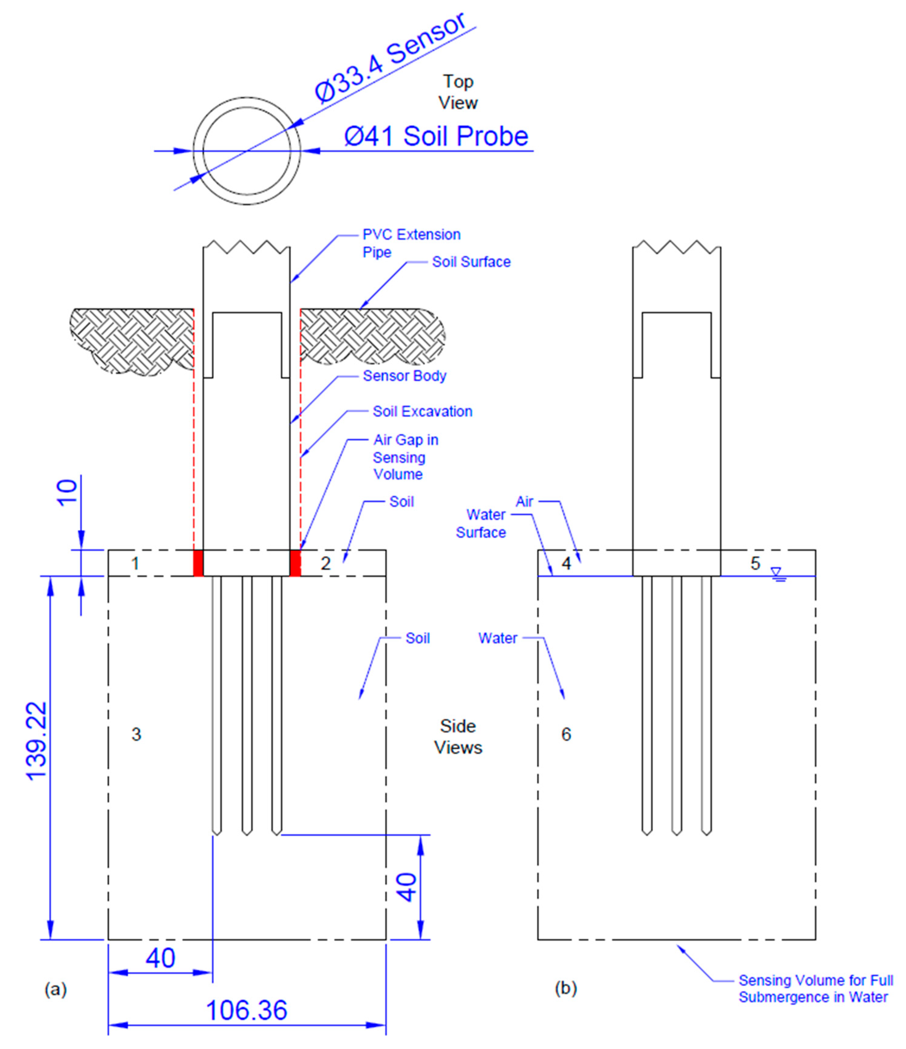
2.1. Description of the Sensor

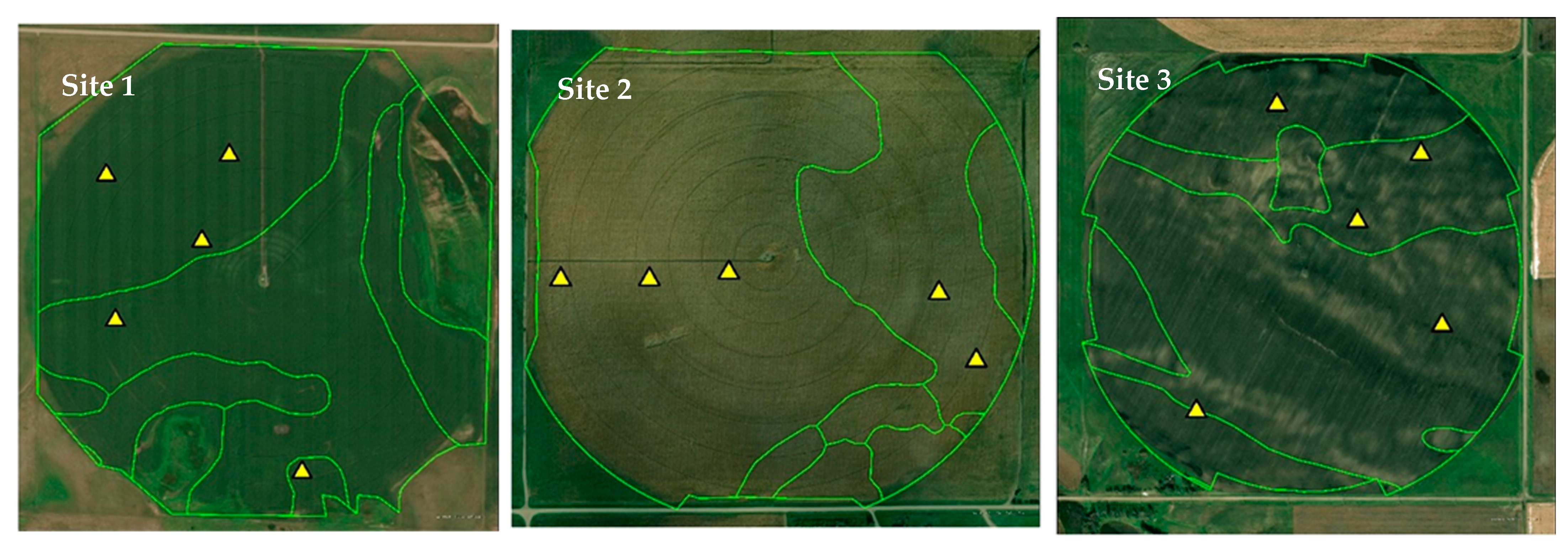
Acclima TDR-310H time-domain reflectometry sensors were used for this study. This sensor model uses three 10 cm waveguides with a rod spacing of 1.14 cm. The waveguides extend from the bottom of the sensor body. We connected the other end of the sensor to a PVC extension pipe with its cable fed up through the pipe into the upper end. The sensor can measure θ_v from 0% to 100% within the operating temperature from −20 °C to 50 °C [18]. We assumed no sensor-to-sensor variability for this study. Sensor data were collected using an Acclima handheld reader (SDI12 Acclima Sensor Reader, Meridian, ID, USA). One reading per depth and station was taken using the reader.

2.2. Field Sites

The soil samples were collected from three sites in southeastern North Dakota, United States. The sites were named as site 1 (46.50407° N, 97.4526° W), site 2 (46.27232° N, 97.8977° W), and site 3 (46.32995° N, 98.249° W). Figure 1 shows a map of North Dakota and the field sites. The sites were selected by the research sponsor (the U.S. Department of Agriculture, Natural Resources Conservation Service) considering factors such as participation in the Environmental Quality Incentives Program for variable-rate irrigation, sites suitable for variable rate irrigation (varying soil textures), and a relatively deep water table that would not interfere with root zone soil water.

Fifteen stations at each field were selected based on relatively uniform spacing throughout the field, soil map units from soil survey geographic database [19], elevation, and a geophysical survey that was conducted in October 2020 [20]. The geophysical survey included DUALEM-21 sensor for electromagnetic induction, a cosmic ray neutron detector, and a gamma-ray spectrometer to characterize soil properties on a spatial basis. Soil samples were collected from each station and tested in the lab for soil properties, namely, pH, cation exchange capacity, electrical conductivity (EC), bulk density, organic matter, soil texture, field capacity, and permanent wilting point. Among the fifteen stations at each site, five stations at each site were chosen for this study based on soil types, elevation, suitability for monitoring variable-rate irrigation zones [21,22], and ease of access to the stations with the sensors and soil probes (Figure 2); and soil samples were collected for calibrating the sensor. The soil textures included sand, sandy loam, sandy clay loam, loamy sand, and loam.

Table 2. Crops grown at sites 1, 2, and 3 in 2021 through 2023.

Year	Site 1	Site 2	Site 3
2021	Corn (Zea mays L.)	Corn	Pinto bean (Phaseolus vulgaris L.)
2022	Corn	Corn	Corn
2023	Pinto bean	Corn	Corn

shows the crops grown in 2021 through 2023.

Table 3. Summary of soil properties at depths of 15 and 46 cm at the five monitoring stations sampled at each field site.

Site #	Statistic	Electrical Conductivity (EC), dS m−1	Field Capacity, cm3 cm−3	Permanent Wilting Point, cm3 cm−3	Bulk Density, g cm−3	Organic Matter, %	% Sand	% Silt	% Clay
1	Average	0.244	0.22	0.13	1.45	1.94	66.2	17	16.8
	Maximum	0.42	0.34	0.22	1.59	3.5	94	26	35
	Minimum	0.11	0.07	0.05	1.36	0.3	44	1	5
2	Average	0.58	0.23	0.13	1.46	2.152	72.8	18.3	9.2
	Maximum	0.81	0.33	0.18	1.58	4.4	84	24	13
	Minimum	0.45	0.17	0.11	1.28	0.22	64	9	4
3	Average	0.59	0.20	0.11	1.53	1.852	74.2	17.8	8
	Maximum	3 1	0.27	0.16	1.78	3.6	84	25	12
	Minimum	0.09	0.13	0.06	1.29	0.26	63	9	3

Note(s): ¹ EC = 3.0 dS m⁻¹ was an outlier; the second largest EC value in the study of [20] was 0.85 dS m⁻¹, at site 2, for a station and depth not used in this paper.

summarizes the soil properties of the five stations for each field site. The soil properties were determined in the Soil Testing Lab and other lab facilities at North Dakota State University, as discussed in [20], where all 15 stations were sampled, but in this paper, the data from only 5 stations per field site were used. Note that the soil samples collected for sensor calibration were taken from the same stations but are not identical to the samples used by [20]. Site 3 had the lowest and highest electrical conductivity (EC) values (0.09 and 3.0 dS m⁻¹, respectively). According to [18], the TDR-310H is suitable for soils with salinity up to 5 dS m⁻¹. The bulk density varied from 1.16 to 1.70 g cm⁻³ with variable soil texture. Organic matter was higher (4.4%) at site 2 compared to site 1 and site 3. The field capacity and permanent wilting point was determined by the pressure plate method. The field capacity and permanent wilting point of all three sites were between 0.34 and 0.05 cm³ cm⁻³, respectively.

2.3. Calibration Protocol

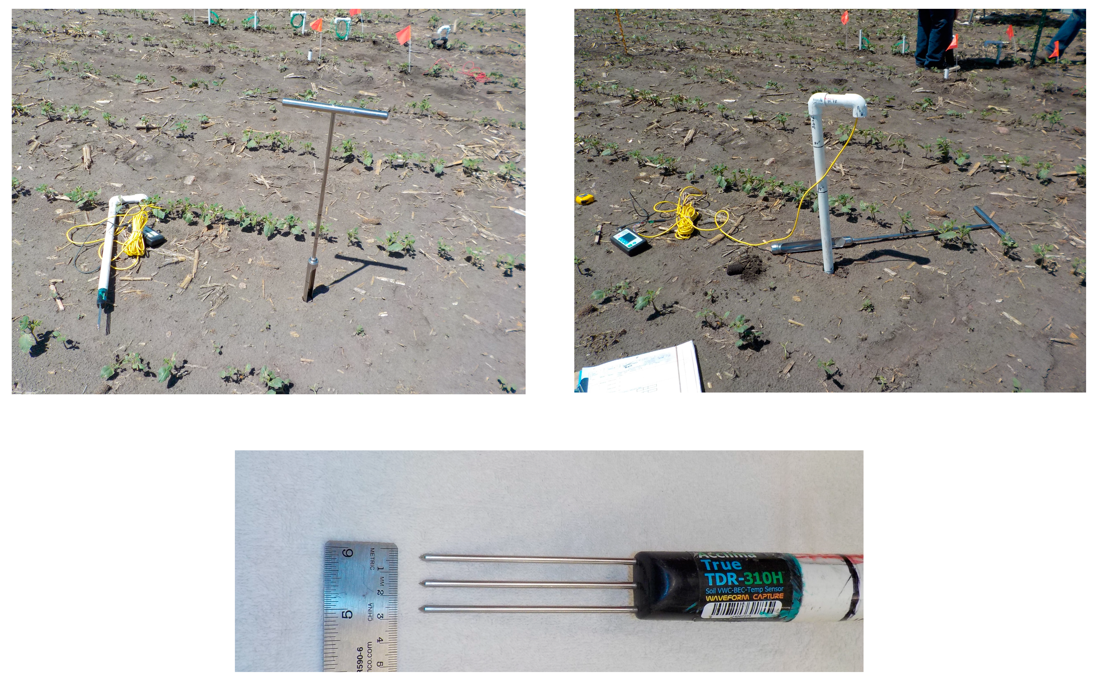
2.3.1. Materials for Soil Sampling

A soil sampling tube (JMC Soil Samplers, model PN055(BC21), Clements Associates Inc., Newton, IA, USA) with an inside diameter of the cutting face 31 mm was used to collect soil samples. Tin sample canisters (Item #77088, Forestry Suppliers, Inc., Jackson, MS, USA) were used to store and transport the samples.

The calibration effort was part of a larger study that used 15 cm, 46 cm, 76 cm, and 106 cm depths for the measurement of soil water content using different sensors. For the calibration, the target depths of 15 cm and 46 cm were considered the centers of 0–30 cm and 30–60 cm soil depths (or the center of each 1-foot depth), respectively. The calibration was not performed for the 76 cm and 106 cm soil depths due to difficulties associated with inserting the sensor and collecting the soil sample. The sampling goal was thus 3 sites × 5 monitoring stations × 2 depths = 30 samples. The limited timeframe, labor, and distance to the field sites prevented us from collecting more soil samples for a full range of calibration curves for each station and depth.

2.3.2. Collection of Soil Samples

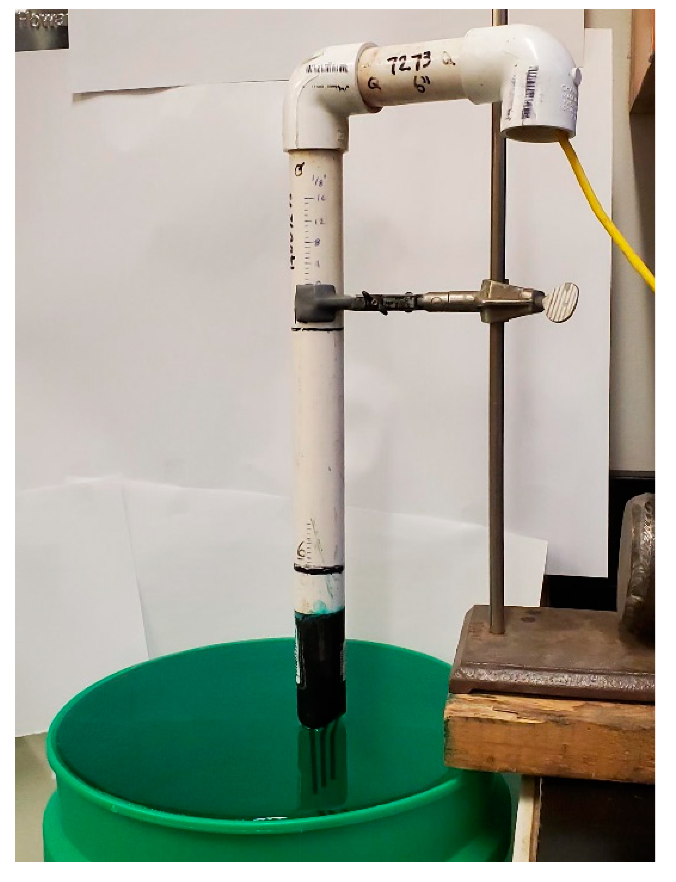
The following procedures were used at each site and station once during the period 3–22 June 2021. Using the above soil sampling tube, a 10 cm long and 3.1 cm diameter soil core was removed by pushing downward, rotating, and then carefully pulling out the sampling tube from the soil. Acclima’s “TDR Probe Guide” was used before inserting the sensor into the soil to make sure the sensor rods/waveguides are not bent or twisted. The TDR Probe Guide ensures the waveguides are parallel. The sensor (mounted on the PVC pipe extension) connected with the Acclima SDI-12 handheld reader (Figure 3) was inserted into the hole, being careful not to twist the sensor, which could introduce air gaps, with the waveguides fully contacting the soil. The handheld reader only reads θ_v and is not programmable with a calibration equation. In the 10 cm hole, the waveguides read from 10 to 20 cm depth, centered at the 15 cm depth. After reading the sensor, it was removed, and the soil sampling tube was inserted to a depth of 10 to 20 cm to capture the soil volume just read by the sensor and care was taken to preserve bulk density as much as possible. It should be noted that the sampling tube was cored to some extra length to ensure capture of the full length of the sample from which the 10 to 20 cm section of soil was sliced for calibration. The process was repeated for the samples centered at 46 cm depth. The length and diameter of each undisturbed sample was 10 cm and 31 mm, respectively, determined by the soil sampling tube, thus giving a fixed volume of the sample. Immediately after removal from the soil profile, each soil sample was emptied into a manila folder and slid into a tin sample canister. The canisters were sealed with polyvinyl chloride electrical tape (model DNFG-34ET, Menards, Eau Claire, WI, USA) in the field to minimize water loss during transport to the lab. The samples were then oven dried at 105–110 °C for a minimum of 24 h to determine gravimetric water content (θ_g, g g⁻¹; [23]). Values of θ_v were determined as θ_g × ρ_b/ρ_w, where ρ_b is the bulk density (g cm^–3) based on soil core volumes and assuming a unit density of water for ρ_w.

In some cases, it was difficult to insert the soil tube at 46 cm depth because of coarse-textured soil. At one of the stations at site 2, a 15 cm sample was obtained, but the soil could not be cored at 46 cm. So, sampling was restarted another day, including the calibration for 15 cm and 46 cm depth, resulting in two replications of 15 cm depth. At site 3, gravel was encountered at 46 cm at two stations and soil samples could not be obtained. As a result of these sampling difficulties, there were 29 samples instead of the 30-sample goal.

Soil cores were carefully collected taking the sensing volume of the sensor into consideration. An engineer at Acclima tested the sensor in water at shallower depths. He submerged the horizontal Acclima TDR sensor and slowly raised it toward the water surface, noting when the sensor started to detect the air boundary. The distance he found was 14 mm from the sensor center rod [24]. The highest sensitivity lies in that 14 mm region, and our soil sample of 10 cm length and 31 mm diameter includes that volume. Figure 4 shows an example of the three waveguide holes that were centered in a soil core that considered the sensor’s maximum sensitivity surrounding the waveguides. Selection of this sampling volume is anticipated to be advantageous compared with soil coring adjacent to the sensor because the spatial offset is negligible.

2.3.3. Calibration

The θ_v readings were collected from the three sites and compared with the θ_v from the lab measurements. The TDR data (θ_v-TDR) and sample data (θ_v-Sample) were pooled together to develop one calibration equation for three sites. A calibration equation was developed from the linear relationship between the field and lab measurements, and confidence intervals for slope and intercept were determined.

To test the robustness of the calibration equation across soil heterogeneity, we tested EC, clay content, and OM as possibly causing larger residual error (RE) (RE corresponds with sensor reading deviations from the producer calibration equation’s estimates of sample volumetric water content) for some soil texture(s) more than the others. (“Producer” and “user” equations are complementary or inversed forms of the calibration equation and are discussed later.) We calculated the correlation (coefficient of determination, R²) of RE between sensor readings and θ_v against EC, clay content, and OM, using data reported by [20], to identify whether a soil-specific calibration might have been helpful instead of pooling the data. This analysis may help determine whether a unified calibration model could effectively account for these key variables across the soil types used in this study or if individual calibrations for each soil type would provide more accurate results.

Additional testing was conducted in the lab to assess the influence of possible small air gaps surrounding the sensor body during the in situ calibration process. This concern is addressed because a soil sampling tube slightly larger than the sensor and extension pipe (41 mm vs. 33.4 mm, respectively) was used for ease of inserting the sensor. To minimize air gaps, a drill bit auger with the same diameter as the sensor could have been used. However, to insert the sensor, especially to reach the deeper depth through the same diameter hole, water might have been needed to act as a lubricant, which would have affected the calibration. Air gaps are depicted in Figure 5a as the red annular space around the bottom or tip of the sensor body. Ref. [25], an updated version of [18], adds information about the sensor's sensing volume, suggesting that the sensing volume for the Acclima TDR-310H sensor corresponds with a θ_v reading of 1.00 cm³ cm⁻³ under conditions of full immersion in water, namely, “at least 4 cm of water around the rods on all sides, beyond the tips of the rods, and at least 1 cm of the sensor body immersed”. This sensing volume is depicted in Figure 5a. For purposes of discussion, the 1 cm of sensor body immersion is denoted herein as the “head space sensing volume” and is labeled as regions 1 and 2 (plus the red regions) in Figure 5a, or regions 4 and 5 in Figure 5b.

The assessment of air gaps in the head space sensing volume on the θ_v readings was accomplished by taking sensor readings at successively deeper depths below a free water surface. The sensor body was partially lowered into a water surface using a pail of water in the lab, as shown in Figure 6, taking care to meet the clearance requirements of the sensing volume. We took three sets of 17 measurements of θ_v from 0 to 5.1 cm of immersion, measured from the water surface to the bottom of the sensor body, in 0.3-cm (1/8-inch) increments. The first reading at the water surface, denoted as 0 cm depth, was ignored because surface tension drew water to the sensor body before the latter was lowered to the water surface elevation.

2.3.4. Validation

Another set of field measurements was collected from 25 May to 15 June 2023 to validate or confirm the calibration equation. A similar procedure as in 2021 was used to collect the data. Readings of θ_v from the sensor were collected from the same locations in each of the three field sites and compared with the θ_v from the lab measurements. A 95% confidence interval was calculated to determine whether the 2023 slope and intercept values lay within the bounds of the 2021 confidence intervals.

2.4. Statistical Analyses

A linear calibration equation was developed using the following calibration equation:

$${\mathsf{\theta }}_{\text{v-Sample}}=\mathrm{a}+\mathrm{b}{\mathsf{\theta }}_{\text{v-TDR}},$$

(1)

where θ_v-Sample is the θ_v obtained from the gravimetric method, θ_v-TDR is the θ_v obtained from the sensor, and a and b are intercept and slope, respectively.

Three statistical measurements were used to quantify the difference between gravimetric soil sample taken from the field and the sensor readings. These are mean bias error (MBE), root mean square error (RMSE), and coefficient of determination (R²). The MBE is given by the following:

$$\mathrm{M}\mathrm{B}\mathrm{E}={\displaystyle \frac{1}{\mathrm{n}}}{\sum }_{\mathrm{i}=1}^{\mathrm{n}}\left({\mathsf{\theta }}_{\text{v-TDR}}-{\mathsf{\theta }}_{\text{v-Sample}}\right),$$

(2)

where n is the total number of samples. A positive bias error means the sensor overestimated the θ_v and a negative bias error means the sensor underestimated the water content measurement. The RMSE and R² values are given by the following:

$$\mathrm{R}\mathrm{M}\mathrm{S}\mathrm{E}=\sqrt{{\displaystyle \frac{1}{\mathrm{n}}}{\sum }_{\mathrm{i}=1}^{\mathrm{n}}{\left({\mathsf{\theta }}_{\text{v-TDR}}-{\mathsf{\theta }}_{\text{v-Sample}}\right)}^2},$$

(3)

$${\mathrm{R}}^2=1-{\displaystyle \frac{{\sum }_{\mathrm{i}=1}^{\mathrm{n}}({{\mathsf{\theta }}_{\text{v-TDR}}-{\mathsf{\theta }}_{\text{v-Sample}})}^2}{{\sum }_{\mathrm{i}=1}^{\mathrm{n}}{\left({\overline{\mathsf{\theta }}}_{\text{v-Sample}}-{\mathsf{\theta }}_{\text{v-Sample}}\right)}^2}},$$

(4)

where ${\overline{\mathsf{\theta }}}_{\text{v-Sample}}$ is the mean of the θ_v-Sample values. The formulas for MBE, RMSE, and R² were used following the studies of [26,27,28].

Probability statistics were used to test two hypotheses. Here, a t-test was used as the sample size (n) was small (n < 30) [29]. The null and alternative hypotheses are shown in

Table 4. Slope and intercept of null and alternative hypotheses.

Parameters	Intercept	Slope
Ho = null hypothesis	a = 0	b = 1
Ha = alternative hypothesis	a ≠ 0	b ≠ 1

.

The confidence interval for the slope is given by [30] the following:

$$\mathrm{b}\pm t_{\alpha /2,n-2}\ast S_e\sqrt{{\displaystyle \frac{n}{S_{xx}}}},$$

(5)

and for the intercept, it is as follows:

$$\mathrm{a}\pm t_{\alpha /2,n-2}\ast S_e\sqrt{{\displaystyle \frac{S_{xx}+{\left(n\overline{x}\right)}^2}{n{S}_{xx}}}}.$$

(6)

Considering a 95% confidence limit, α is the desired significance level and t_α/2 is the 100(1−α/2) percentile of t distribution with n − 2 degrees of freedom. The standard error of estimate is S_e and $\overline{x}$ is the sample mean (θ_v-TDR). The t statistics were calculated to test the hypotheses and to analyze the need for a field calibration for the soil water sensor. If the 95% confidence intervals include 0 for the intercept and 1 for the slope, it means that the factory calibration equation can be used for field use of the Acclima TDR-310H sensor. Otherwise, a field calibration equation will be needed.

The Equation (1) used here is named as a “users’ calibration equation” or the inversed form [14] of the typical calibration equation, θ_v-TDR = b + aθ_v-Sample. Here, users are people using the sensor in the field. Gravimetric θ_v-Sample can be estimated from the θ_v-TDR using Equation (1). The statistics used in this study are derived from the users’ calibration equation. Since users are typically individuals conducting field measurements, having a calibration equation developed to their specific conditions enables them to use the sensor effectively in production settings. This ensures that the readings obtained are reliable and reflective of the soil moisture conditions on-site. However, the charts presented here are based on a “producers’ calibration equation”, where producers are sensor manufacturers who show how a sensor reports known soil water content (θ_v-TDR on y-axis and θ_v-Sample on x-axis). Using a producer chart with a 1:1 line, readers can easily see sensor under- or over-estimation of θ_v compared with the referenced θ_v.

3. Results and Discussion

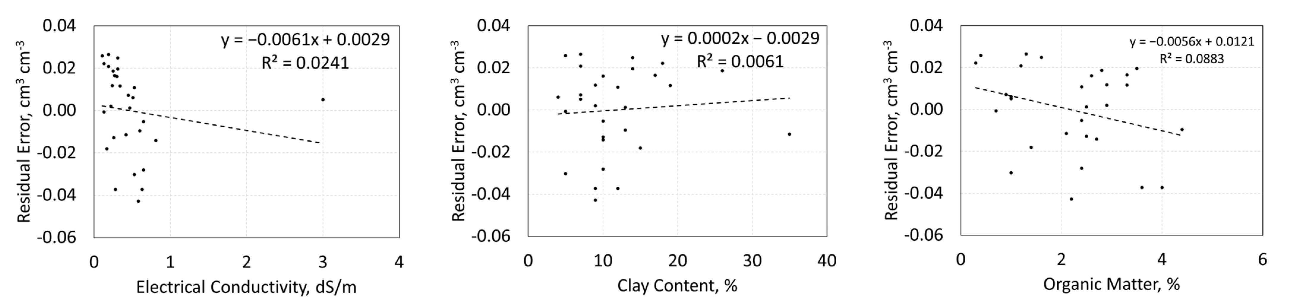
3.1. Residual Error Dependency on Soil Properties

Correlations between RE and EC, clay content, and OM were tested (Figure 7). The R² values were 0.0024 for RE vs. EC, 0.0061 for RE vs. clay content, and 0.088 for RE vs. OM. These results suggest that EC, OM, and clay content had weak influences on the residual errors. For further understanding of whether the slopes significantly differ from zero, p-values for the slopes were calculated. The p-value for the RE vs. EC slope was 0.42; for RE vs. clay content, it was 0.69; and for RE vs. OM, it was 0.12; all of the p-values were greater than 0.05, meaning that the slopes of the regression curves are not significantly different from zero. The data were randomly scattered (Figure 7), so modeling of the non-linear trends was not conducted.

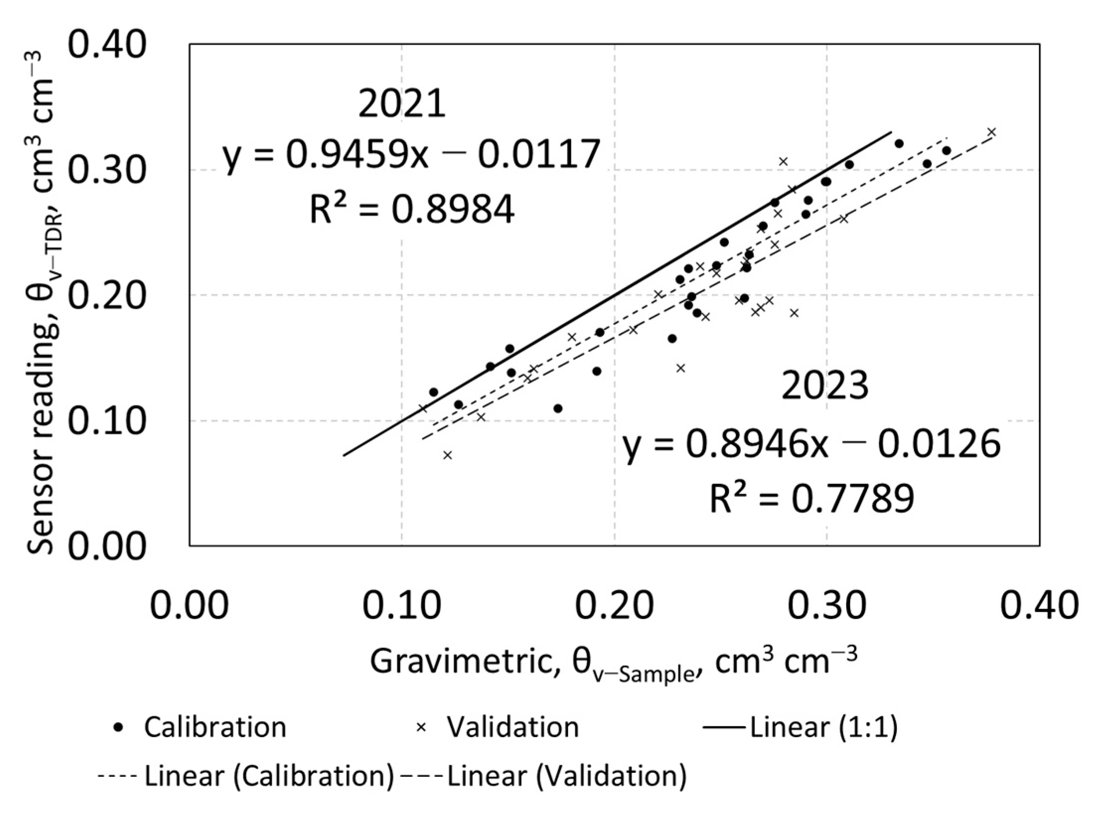
3.2. Calibration Statistics

The producers’ calibration generated a slope of 0.95 and an intercept of −0.012 cm³ cm⁻³ (Figure 8). The R² of linear regression was 0.90. The slope of the sensor was compared with a linear 1:1 line to show the correlation between the sensor readings with the changing soil water content. The chart is suitable for manufacturers reporting the accuracy of their sensors using the given equation. In general, the sensor underestimated the θ_v-Sample values. On three instances, or ~10% of the time, the sensor overestimated the θ_v-Sample values, but this did not show any correlation with higher clay content or higher salinity (higher EC); that is, the overestimation is attributed to random scatter in the data.

Feng and Sui [7] found that the Acclima TDR-315 sensor underestimated θ_v by an average of 0.04 cm³ cm⁻³ in the 0–15 cm of layers of Brooksville silty clay during an off-season field test. They identified the inaccuracies associated with the higher clay content of the soil. In our study, the Acclima TDR-310H sensor underestimated the θ_v-Sample, and possible reasons could be air pockets or pore space in the dry soil, the slight disturbance of the surrounding soil while installing the sensor, or soil compaction due to inserting the soil sampling tube into the soil [31]. While some degree of compaction is largely unavoidable during the soil coring operations, we tried to keep the soil sample as undisturbed as possible.

In addressing air gaps around the sensor body, we first note that the sensor accuracy is ±0.03 cm³ cm⁻³ [25] and that the Acclima TDR reader display gives θ_v as a percentage with two decimal places, such as 98.43%, which we convert to cm³ cm⁻³ here. Sensor readings averaged 0.9843 cm³ cm⁻³ for three replications of measurements at immersion depths of 2.5 to 5.1 cm and 0.9821 cm³ cm⁻³ for three replications of immersion depths of 0.3 to 0.6 cm. The difference in the groups of readings, attributable to partial immersion and detection of air, is 0.0021 cm³ cm⁻³ (after rounding), which is an order of magnitude smaller than the sensor accuracy. Furthermore, regions 1 and 2 in Figure 5a were occupied by soil during the field calibration procedure, the water in which was thus presumably detectable by the sensor. In contrast, comparable regions 4 and 5 in Figure 5b during testing in water were occupied only by air. Therefore, the difference between shallow and fully immersed readings in the soil during the field calibration procedure is anticipated to be smaller compared with the same situation in the air-water configuration. The above analysis suggests that although small annular air gaps around the end of the sensor body were introduced as a by-product of the field sampling procedure, they had negligible effects on θ_v readings in the region of the waveguides (regions 3 and 6 in Figure 5a and Figure 5b, respectively).

Table 5. Statistical analyses of calibration results.

Statistics	Bias Error cm3 cm−3	Absolute Error cm3 cm−3
Mean	−0.025	0.026
Maximum	0.008	0.064
Minimum	−0.064	0.001
Standard Deviation	0.021	0.020
Coefficient of Variation %	−84	75

summarizes this study’s bias errors and absolute errors. The RMSE value for this study was 0.032 cm³ cm⁻³, which was smaller than the acceptable RMSE value defined by [3] at 0.035 cm³ cm⁻³ for TDT sensor and [32] at 0.04 cm³ cm⁻³. Refs. [33,34,35] also found similar results with TDR-315 sensor on sandy loam soil. On the other hand, refs. [8,36] found that the Acclima TDR-315 sensor overestimated θ_v in a clayey soil.

The inverse form of the calibration (or user’s calibration) was calculated as θ_v-Sample = 0.95 θ_v-TDR + 0.036, with R² = 0.90. t distribution statistics were applied to test the user’s calibration results. For the n = 29 samples, the degrees of freedom (df) were n − 2 = 27. For a 95% confidence interval, the α was 0.05. Using a t distribution table, the value for t distribution probability t_α/2 is 2.05 for 27 df. From Equations (5) and (6), the confidence intervals for slope and intercept were 0.82 to 1.08 and 0.0072 to 0.064 cm³ cm⁻³, respectively. Because the confidence interval for the slope includes 1, the null hypothesis (b = 1) (Table 3) cannot be rejected. However, the confidence interval for the intercept does not include the ideal intercept of 0, so the null hypothesis (a = 0) should be rejected in this case; that is, from the calibration analysis, the intercept a ≠ 0. Using the calibration equation only for the slope and not for the intercept is impractical. For clarity and simplicity, we recommend the use of a field calibration if either the slope or the intercept hypothesis tests indicate b ≠ 1 or a ≠ 0.

3.3. Validation of Calibration

According to [7,37], calibration should be validated with field values. To validate the results from 2021, θ_v-TDR values were collected from the sensor in 2023, and θ_v-Sample values were determined from soil samples. Figure 9 shows a comparison of 2021 calibration and 2023 validation results. The slope and intercept from the inversed (user’s) calibration equation were determined and compared with the slope and intercept of the 2021 users’ calibration. The results of the validation sampling effort in 2023 shown in

Table 6. Calibration results from 2021 and validation results from 2023.

Item	Year 2021	2021 95% Confidence Interval		Year 2023
		Minimum	Maximum
Slope	0.950	0.82	1.08	0.871
Intercept, cm3 cm−3	0.0357	0.0072	0.0642	0.0639
No. of samples	29	NA	NA	27
Sample maximum θv	0.36	NA	NA	0.38
Sample minimum θv	0.11	NA	NA	0.11
Sensor maximum θv	0.32	NA	NA	0.33
Sensor minimum θv	0.11	NA	NA	0.07

Note: Abbreviations: θ_v = volumetric water content; NA = not applicable. The 95% confidence intervals were determined only for the slope and intercept.

indicate that the new slope and intercept values (0.8707 and 0.063881, respectively) fall within 95% confidence interval of the 2021 users’ calibration slope and intercept, respectively. Additionally, the R² value of 0.78 suggests a relatively good fit for calibration. In practical terms, this means that the users’ calibration equation established in 2021 remains valid and accurate for the Acclima TDR-310H sensor. Researchers and practitioners can continue to use the calibration equation with confidence when working with these particular soil types.

We acknowledge that the number of soil samples limits the robustness of the calibration equation across many soil types. However, the sampling we conducted represented all of the monitoring stations (soil types) used in this study.

4. Management Implications

This article provides valuable insights for users of soil water sensors, including farmers, growers, or crop consultants, on the importance and process of sensor calibration. By understanding how to calibrate TDR sensors, users can identify and correct errors in sensor readings, especially when dealing with similar soil textures. Utilizing the users’ calibration equation and calibration chart, users can accurately determine the referenced volumetric water content from the sensor readings. For example, as a practical implication of calibration, in Nebraska, USA, researchers [14] found a 56% reduction in the RMSE in silt loam soil and a 28% reduction in loamy sand soil after calibrating a TDR-315L soil water sensor. In a companion study [38], sensor accuracy impacts on management decisions (irrigation triggers, crop evapotranspiration, and total soil water) were evaluated. For example, a calibrated TDR-315L sensor predicted more or fewer irrigation events compared to a reference neutron probe, depending on soil type and growing season.

5. Conclusions

An Acclima TDR-310H soil water sensor was tested and calibrated on multiple field sites with active crop growth to analyze the sensor accuracy in field conditions. The sensor measurement depths were 15 and 46 cm in this study, and soil samples were collected at these depths. On average, the sites contained a high sand percentage, and salinity levels were within the acceptable limit (<5 dS m⁻¹ [18]) for the sensor (but note [25], available after starting this project, lists < 2 dS m⁻¹). The results showed that the sensor underestimated θ_v, which is consistent with other reports from the literature. The MBE (−0.025 cm³ cm⁻³) slightly exceeded the limit set by the manufacturer (±0.02 cm³ cm⁻³), and the RMSE of 0.032 cm³ cm⁻³ was acceptable (<0.04 cm³ cm⁻³).

Linear equations were developed using the data points, and the slope and intercept were calculated. t distribution statistics were applied to identify the confidence intervals for the slope and intercept of the users’ calibration equation. The confidence interval for the slope was 0.82 to 1.08, and for the intercept was 0.0072 to 0.0642 cm³ cm⁻³. As the confidence interval for the slope includes the ideal value of 1.0, the factory calibration could be used on that basis. However, the ideal intercept, a = 0, is not included in the confidence interval, which means the factory calibration should not be used on that basis. Because one of the parameters was outside of its confidence interval, we recommend using the field calibration equation developed in this study. If the factory calibration is used, a user could expect the error to be approximately −0.025 cm³ cm⁻³ (the value of MBE) for these soils. Moreover, the validation results supported that the calibration equation can be used for this sensor with similar soil types.

We acknowledge that a week of acclimation time—or several wetting and drying cycles—before collecting the sensor readings could have been helpful but would not have been feasible in a farmer’s field due to equipment, time, and travel constraints, in addition to the resulting disturbance in the farmers’ fields. On the other hand, the laboratory work showing that air gaps around the sensor head had negligible effects on sensor readings has a practical implication; i.e., it demonstrates that field calibration can be conducted more easily and quickly compared with approaches using sampling techniques involving excavations of soil around the sensor head after typical field installation.

Future studies could include calibrating the sensor in saline soils to identify the threshold for salinity. Additional testing and sensor calibration should be considered for situations involving soils with higher EC, clay content, and/or organic matter than those used in this study. Because of our inability to obtain soil samples in some gravelly locations, future research could assess the correlation of residual errors on the fraction of coarse fragments in the soil.

This paper is a revised and expanded version of our paper published in [39].

References

1. FAO. The Future of Food and Agriculture—Trends and Challenges. Rome 2017. Available online: https://www.fao.org/3/a-i6583e.pdf (accessed on 3 July 2024).
2. Cooley, H.; Christian-Smith, J.; Gleick, P.H. Sustaining California Agriculture in an Uncertain Future; Pacific Institute: Oakland, CA, USA, 2009; Volume 81, Available online: https://pacinst.org/wp-content/uploads/2014/04/sustaining-california-agriculture-pacinst-full-report.pdf (accessed on 2 April 2025).
3. Varble, J.L.; Chávez, J.L. Performance evaluation and calibration of soil water content and potential sensors for agricultural soils in eastern Colorado. Agric. Water Manag. 2011, 101, 93–106. [Google Scholar] [CrossRef]
4. Topp, G.C.; Davis, J.; Annan, A.P. Electromagnetic determination of soil water content: Measurements in coaxial transmission lines. Water Resour. Res. 1980, 16, 574–582. [Google Scholar] [CrossRef]
5. Hignett, C.; Evett, S. Chapter 1: Direct and surrogate measures of soil water content. In Field Estimation of Soil Water Content: A Practical Guide to Methods, Instrumentation and Sensor Technology; Cepuder, P., Evett, S.R., Heng, L.K., Hignett, C., Laurent, J.P., Ruelle, P., Eds.; Training Course Series No. 30; International Atomic Energy Agency: Vienna, Austria, 2008; pp. 1–22. Available online: https://www-pub.iaea.org/mtcd/publications/pdf/tcs-30_web.pdf (accessed on 26 February 2020).
6. Evett, S.R.; Cepuder, P. Chapter 5: Capacitance sensors for use in access tubes. In Field Estimation of Soil Water Content: A Practical Guide to Methods, Instrumentation, and Sensor Technology; Evett, S.R., Heng, L.K., Moutonnet, P., Nguyenm, M.L., Eds.; IAEA-Training Course Series No. 30. International Atomic Energy Agency: Vienna, Austria, 2008; pp. 73–90. Available online: https://www-pub.iaea.org/mtcd/publications/pdf/tcs-30_web.pdf (accessed on 26 February 2020).
7. Feng, G.; Sui, R. Evaluation and calibration of soil moisture sensors in undisturbed soils. Am. Soc. Agric. Biol. Eng. 2020, 63, 265–274. [Google Scholar] [CrossRef]
8. Datta, S.; Taghvaeian, S.; Ochsner, T.E.; Moriasi, D.; Gowda, P.; Steiner, J.L. Performance assessment of five different soil moisture sensors under irrigated field conditions in Oklahoma. Sensors 2018, 18, 3786. [Google Scholar] [CrossRef]
9. Evett, S.R.; Tolk, J.A.; Howell, T.A. Time domain reflectometry laboratory calibration in travel time, bulk electrical conductivity, and effective frequency. Vadose Zone J. 2005, 4, 1020–1029. [Google Scholar] [CrossRef]
10. Quinones, H.; Ruelle, P. Operative Calibration Methodology of a TDR Sensor for Soil Moisture Monitoring under Irrigated Crops. Subsurf. Sens. Technol. Appl. 2001, 2, 31–45. [Google Scholar] [CrossRef]
11. Birendra, K.C.; Chau, H.W.; Mohssen, M.; Cameron, K.; Safa, M.; Mclndoe, I.; Rutter, H.; Dark, A.; Lee, M.; Pandey, V.P.; et al. Assessment of spatial and temporal variability in soil moisture using multi-length TDR probes to calibrate Aquafex sensors. Irrig. Sci. 2021, 39, 703–713. [Google Scholar] [CrossRef]
12. Jia, J.; Zhang, P.; Yang, X.; Zhen, Q.; Zhang, X. Comparison of the accuracy of two soil moisture sensors and calibration models for different soil types on the loess plateau. Soil Use Manag. 2020, 37, 584–594. [Google Scholar] [CrossRef]
13. Kim, K.; Sim, J.; Kim, T.H. Evaluation of the effects of soil properties and electrical conductivity on the water content reflectometer calibration for landfill cover soils. Soil Water Res. 2017, 12, 10–17. [Google Scholar] [CrossRef]
14. Sharma, K.; Irmak, S.; Kukal, M.S.; Vuran, M.C.; Jhala, A.; Qiao, X. Evaluation of soil moisture sensing technologies in silt loam and loamy sand soils: Assessment of performance, temperature sensitivity, and site—And sensor—Specific calibration functions. Trans. ASABE 2021, 64, 1123–1139. [Google Scholar] [CrossRef]
15. Xiao, K.; Bai, W.; Wang, S. Multifactor analysis of calibration and service quality of the soil moisture sensor applied in subgrade engineering. Adv. Mater. Sci. Eng. 2021, 7548996. [Google Scholar] [CrossRef]
16. Zhu, Y.; Irmak, S.; Jhala, A.J.; Vuran, M.C.; Diotto, A. Time-domain and frequency-domain reflectometry type soil moisture sensor performance and soil temperature effects in fine- and coarse-textured soils. Appl. Eng. Agric. 2019, 32, 117–134. [Google Scholar] [CrossRef]
17. Singh, J.; Heeren, D.M.; Rudnick, D.R.; Woldt, W.E.; Bai, G.; Ge, Y.; Luck, J.D. Soil structure and texture effects on the precision of soil water content measurements with a capacitance based electromagnetic sensor. Trans. ASABE 2020, 63, 141–152. [Google Scholar] [CrossRef]
18. Acclima. Data Sheet: True TDR-310H Soil Water-Temperature-BEC Sensor; Acclima, Inc.: Meridian, ID, USA, 2019; Available online: https://acclima.com/wp-content/uploads/Acclima-TDR310H-Data-Sheet.pdf (accessed on 25 February 2021).
19. Soil Survey Staff, Natural Resources Conservation Service, United States Department of Agriculture. Web Soil Survey. Available online: https://websoilsurvey.nrcs.usda.gov/app/ (accessed on 27 March 2021).
20. Becker, S.M.; Franz, T.E.; Abimbola, O.; Steele, D.D.; Flores, J.P.; Jia, X.; Scherer, T.F.; Rudnick, D.R.; Neale, C.M.U. Feasibility assessment on use of proximal geophysical sensors to support precision management. Vadose Zone J. 2022, e20228. [Google Scholar] [CrossRef]
21. Neale, C.M.U.; (University of Nebraska-Lincoln, Lincoln, NE, USA). Personal communication, 2020.
22. Franz, T.; (University of Nebraska-Lincoln, Lincoln, NE, USA). Personal communication, 2021.
23. Gardner, W.H. Water content. In Methods of Soil Analysis, Part 1: Physical and Mineralogical Methods, 2nd ed.; Klute, A., Ed.; Agronomy No. 9; ASA and SSSA: Madison, WI, USA, 1986; pp. 635–662. [Google Scholar]
24. Anderson, J.; (Acclima Inc., Meridian, ID, USA). Personal communication, 2022.
25. Acclima. Data Sheet: True TDR-310H Soil Water-Temperature-BEC Sensor; Acclima, Inc.: Meridian, ID, USA, 2023; Available online: https://acclima.com/digital-tdr-soil-moisture-sensors/ (accessed on 2 April 2025).
26. Willmott, C.J.; Matsuura, K. Advantages of the mean absolute error (MAE) over the root mean square error (RMSE) in assessing average model performance. Clim. Res. 2005, 30, 79–82. [Google Scholar] [CrossRef]
27. Chicco, D.; Warrens, M.J.; Jurman, G. The coefficient of determination R-squared is more informative than SMAPE, MAE, MAPE, MSE and RMSE in regression analysis evaluation. PeerJ Comput. Sci. 2021, 7, e623. [Google Scholar] [CrossRef] [PubMed]
28. Avdeef, A. Do you know your r2? ADMET DMPK 2021, 9, 69–74. [Google Scholar] [CrossRef]
29. Abebe, T.H. The Derivation and Choice of Appropriate Test Statistic (Z, t, F and Chi-Square Test) in Research Methodology. Math. Lett. 2019, 5, 33. [Google Scholar] [CrossRef]
30. Johnson, R.A. Miller and Freund’s Probability and Statistics for Engineers, 6th ed.; Prentice-Hall, Inc.: Englewood Cliffs, NJ, USA, 2000. [Google Scholar]
31. Evett, S.; (USDA-ARS, Bushland, TX, USA). Personal communication, 2022.
32. Cosh, M.H.; Ochsner, T.E.; McKee, L.; Dong, J.; Basara, J.B.; Evett, S.R.; Hatch, C.E.; Small, E.E.; Steele-Dunne, S.C.; Zreda, M.; et al. The soil moisture active passive arena, Oklahoma, in situ sensor testbed (SMAP-MOISST): Testbed design and evaluation of in situ sensors. Vadose Zone J. 2016, 15. [Google Scholar] [CrossRef]
33. Adeyemi, O.; Norton, T.; Grove, I.; Peets, S. Performance Evaluation of Three Newly Developed Soil Moisture Sensors. In Proceedings of the CIGR-AgEng Conference, Aarhus, Denmark, 26–29 June 2016; Available online: https://conferences.au.dk/uploads/tx_powermail/olutobi_cigr_paper.pdf (accessed on 2 April 2025).
34. Singh, J.; Lo, T.; Rudnick, D.R.; Dorr, T.J.; Burr, C.A.; Werle, R.; Muñoz-Arriola, F. Performance assessment of factory and field calibrations for electromagnetic sensors in a loam soil. Agric. Water Manag. 2018, 196, 87–98. [Google Scholar] [CrossRef]
35. Chávez, J.L.; Evett, S. Using soil water sensors to improve irrigation management. In Proceedings of the 24th Annual Central Plains Irrigation Conference, Colby, KS, USA, 21–22 February 2012; Available online: https://web.archive.org/web/20170603022742/https://www.ksre.k-state.edu/irrigate/oow/p12/Chavez12.pdf (accessed on 2 April 2025).
36. Ferrarezi, R.S.; Nogueira, T.A.R.; Zepeda, S.G.C. Performance of soil moisture sensors in Florida Sandy Soils. Water 2020, 12, 358. [Google Scholar] [CrossRef]
37. Rowlandson, T.L.; Berg, A.A.; Bullock, P.R.; Ojo, E.R.; McNairn, H.; Wiseman, G.; Cosh, M.H. Evaluation of several calibration procedures for a portable soil moisture sensor. J. Hydrol. 2013, 498, 335–344. [Google Scholar] [CrossRef]
38. Sharma, K.; Irmak, S.; Kukal, M.S. Propagation of soil moisture sensing uncertainty into estimation of total soil water, evapotranspiration and irrigation decision-making. Agric. Water Manag. 2021, 243, 106454. [Google Scholar] [CrossRef]
39. Maisha, R.M.; Steele, D.D. Field Calibration of a Time Domain Reflectometry Sensor with an Extension Pipe for Soil Water Content Measurement. In Proceedings of the ASABE Annual International Meeting, Houston, TX, USA, 20 July 2022; ASABE Paper No. 2201013; ASABE: St. Joseph, MI, USA, 2022. [Google Scholar] [CrossRef]
Figure 1. Location of the field sites in Southeast North Dakota.
Water 17 01203 g001
Figure 2. From left to right—geospatial imagery of site 1, 2, and 3, respectively, where yellow triangles represent five stations in each field site which are the soil sampling locations. Green lines represent different soil map units within each field. Field site latitudes and longitudes are as follows: site 1: 46.504066° N, 97.452575° W; site 2: 46.272316° N, 97.897682° W; and site 3: 46.329951° N, 98.249031° W. All irrigation systems fit within 805-m × 805-m square land parcels (U.S. quarter-section land parcels).
Water 17 01203 g002
Figure 3. Soil coring tube used to remove the surface 10 cm of soil (top left); taking volumetric water content reading with the sensor (top right); and close-up view of the sensor head with extension pipe attached (bottom).
Water 17 01203 g003
Figure 4. Soil core with three waveguide holes from the Acclima TDR-310H sensor.
Water 17 01203 g004
Figure 5. Sensor configurations for (a) the sensor in a calibration borehole in field soil, and (b) sensor waveguides submerged in water with the sensor body even with the water surface. Sensor sizes and sensing volumes are the same for (a,b); all dimensions are mm. Except for the sensor waveguides, all features in (a) or (b) may be rotated about a vertical center axis to create cylindrical objects such as the sensor body, the sensing volume, etc. Phantom lines represent sensing volumes derived from [25]. Numbered regions 1–3 and 4–6 comprise the sensing volumes in (a) and (b), respectively. Numbered regions 1 and 2 (plus the red regions) in (a) and regions 4 and 5 in (b) represent head space sensing volumes, respectively.
Water 17 01203 g005
Figure 6. Laboratory setup for testing sensor readings with the sensor body at successively deeper immersion depths.
Water 17 01203 g006
Figure 7. From left to right, correlation between residual error and electrical conductivity, clay content, and organic matter. Dots represent data points and dotted lines represent linear trendlines from least-squares linear regression.
Water 17 01203 g007
Figure 8. Producer calibration chart for 2021 growing season.
Water 17 01203 g008
Figure 9. Comparison of Acclima TDR-310H for the 2021 producers’ calibration and 2023 validation.
Water 17 01203 g009