
An Integrated Approach for Groundwater Potential Prediction Using Multi-Criteria and Heuristic Methods

 , ,
, ,  , , and
Abstract
:1. Introduction
Literature Review
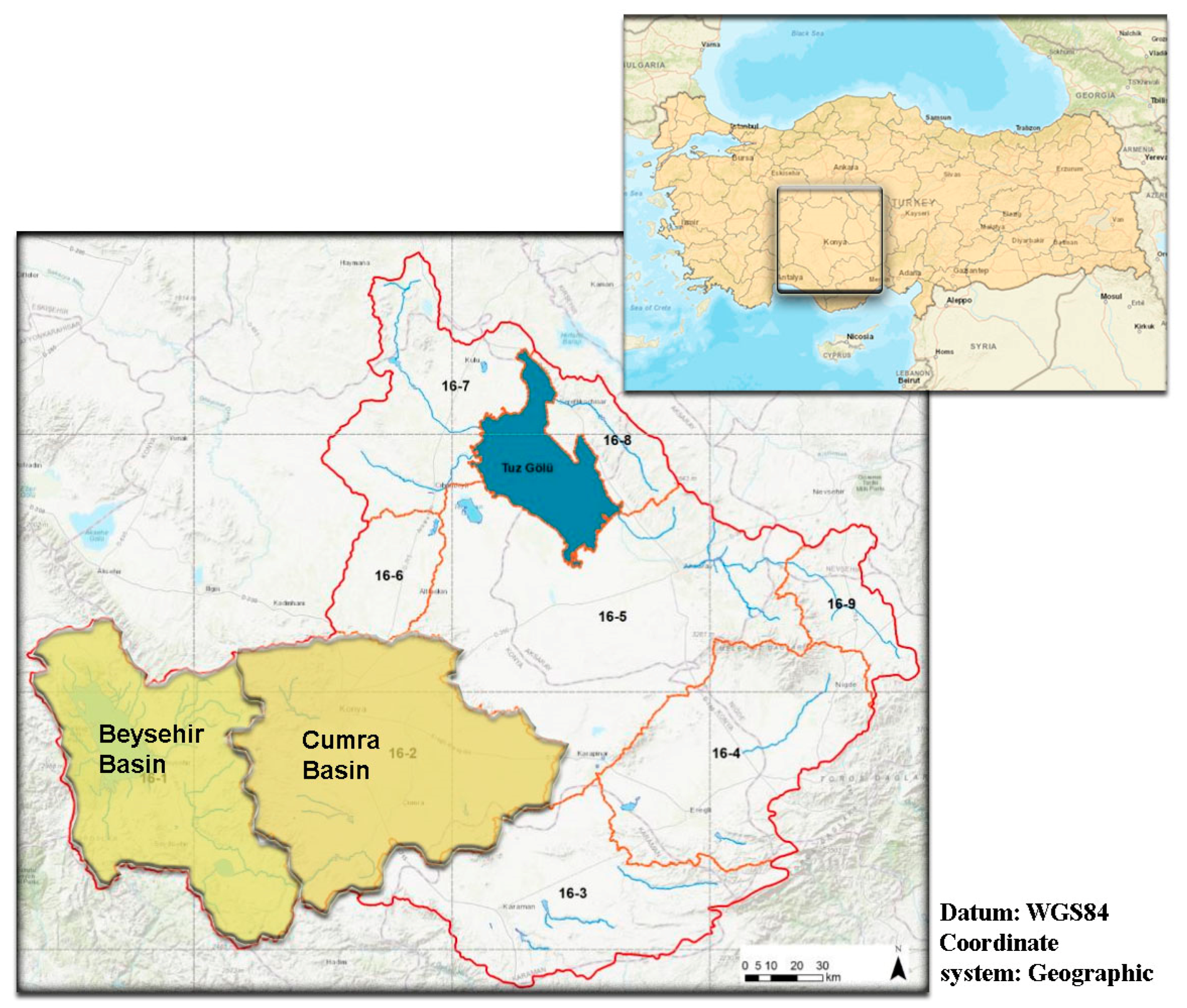
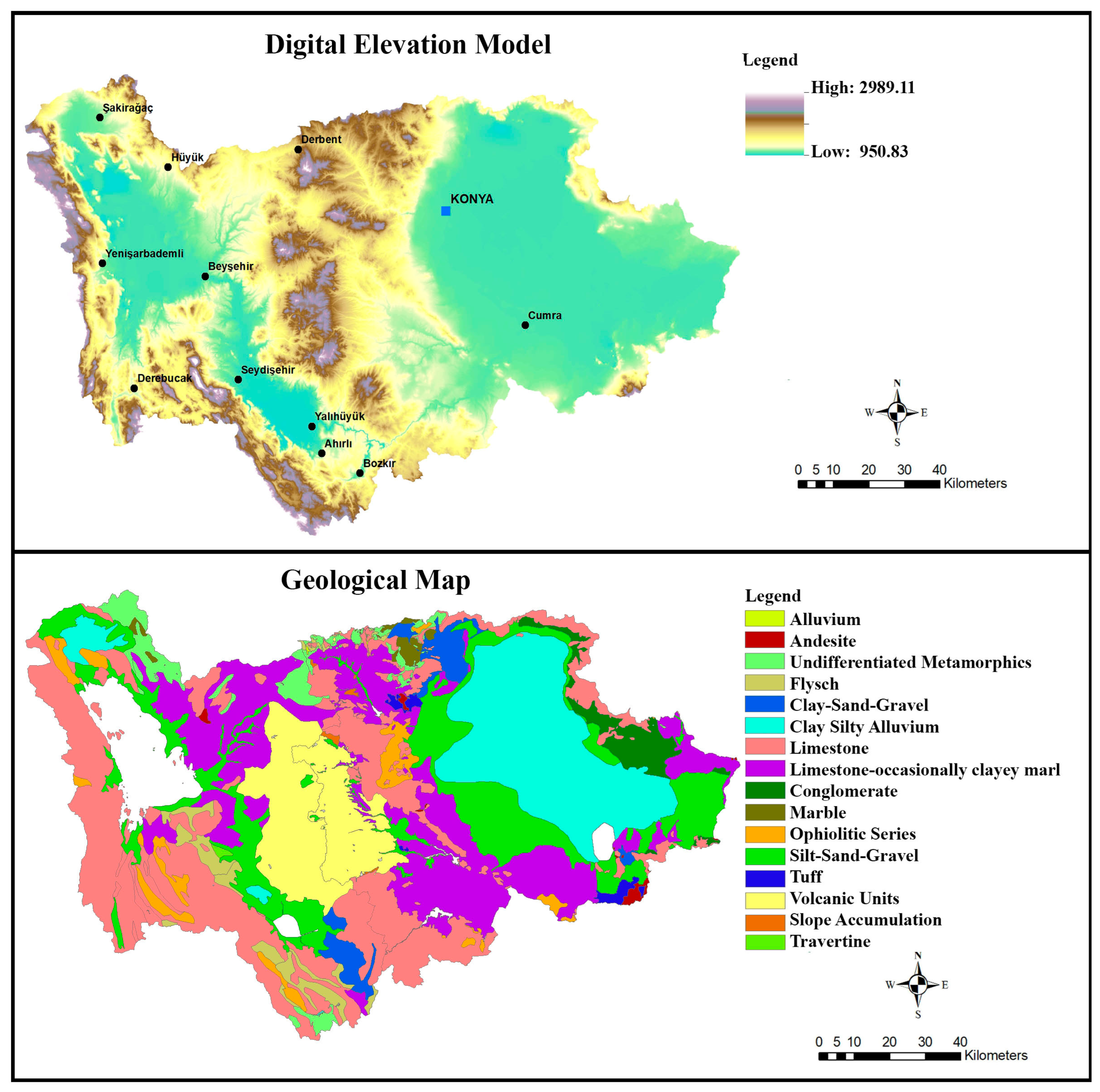
2. Study Area
3. Materials and Methods
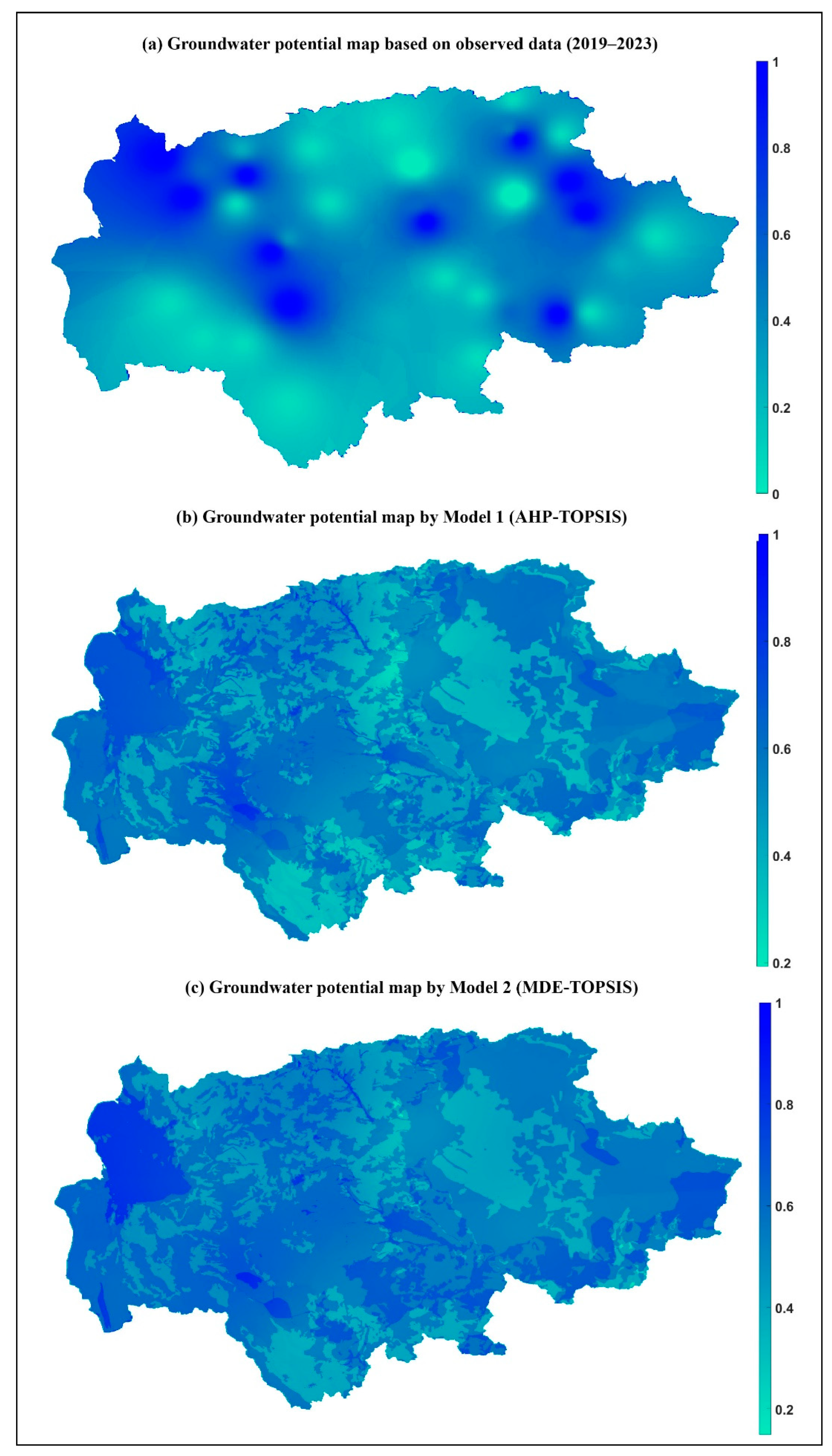
- In Model 1, the groundwater conditioning factors were weighted with the AHP technique, which is one of the expert opinion-based MCDM techniques, and priority ranking was created using the TOPSIS technique.
- In Model 2, the groundwater conditioning factors were weighted with the MDE technique, which is one of the heuristic techniques, and priority ranking was created using the TOPSIS technique.
- The accuracy of Model 1 and Model 2 results was tested by comparing them with the groundwater distribution map produced from data obtained by measuring groundwater levels in drilled wells for the last five years (2019–2023).
3.1. Dataset Description
3.2. Dataset Collection
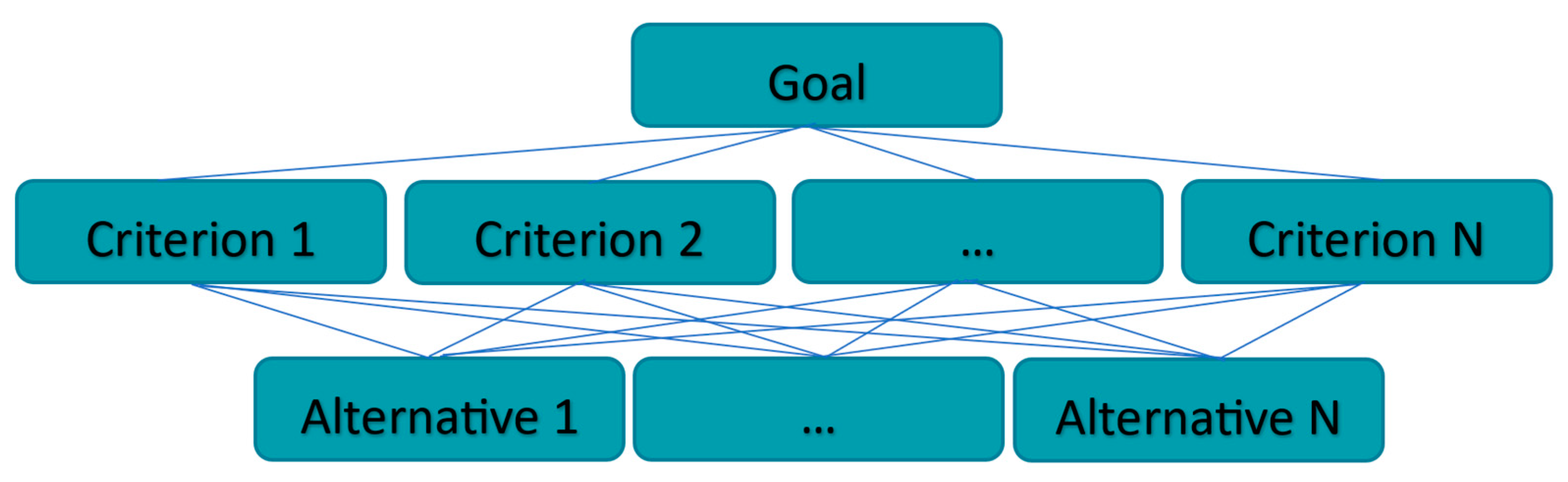
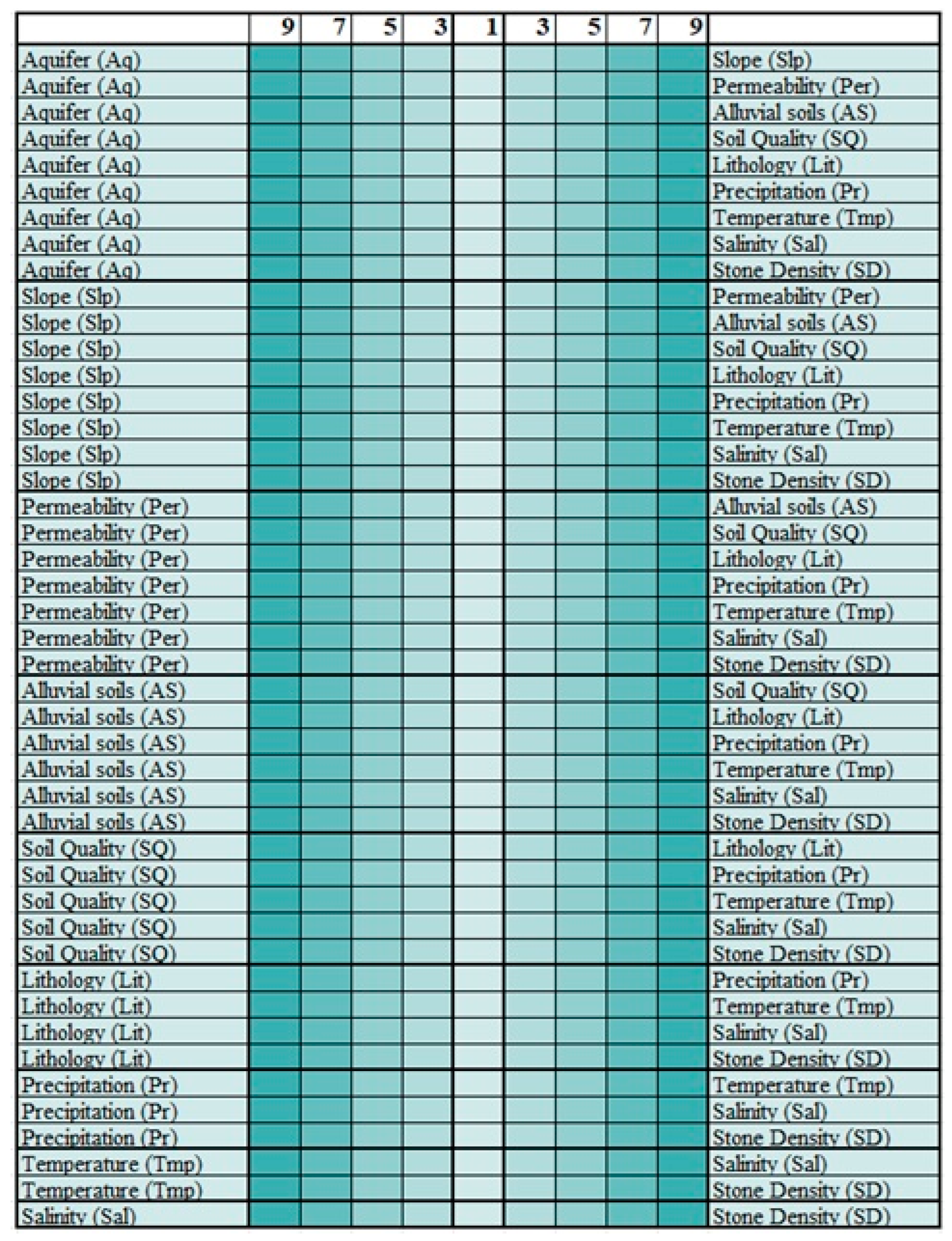
3.3. AHP Method

| N | 1 | 2 | 3 | 4 | 5 | 6 | 7 | 8 | 9 | 10 |
| RI | 0 | 0 | 0.58 | 0.9 | 1.12 | 1.24 | 1.32 | 1.41 | 1.45 | 1.49 |
3.4. TOPSIS Method
3.5. Heuristic Algorithms
Multi-Population-Based Differential Evolution Algorithm (MDE)
4. Results
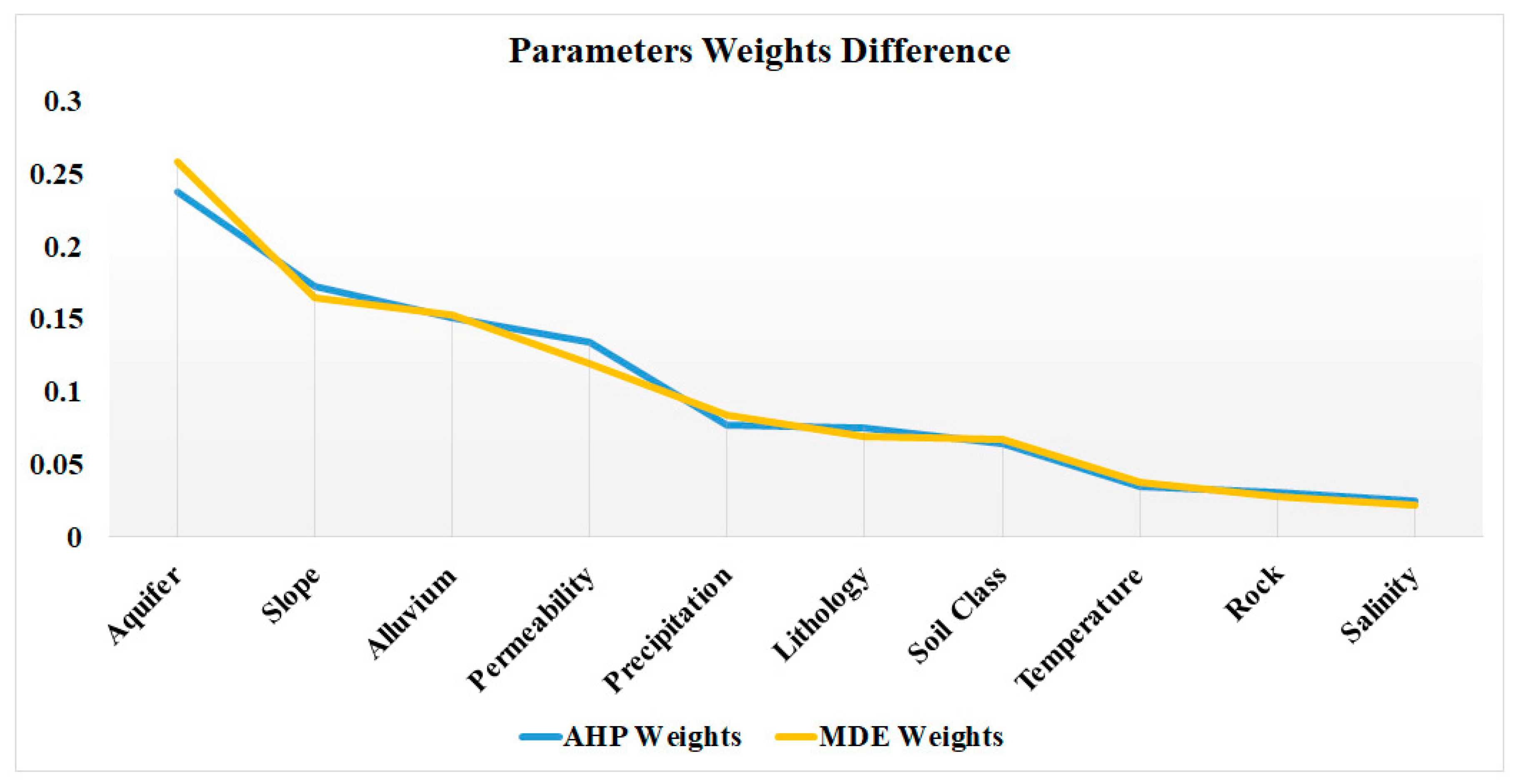
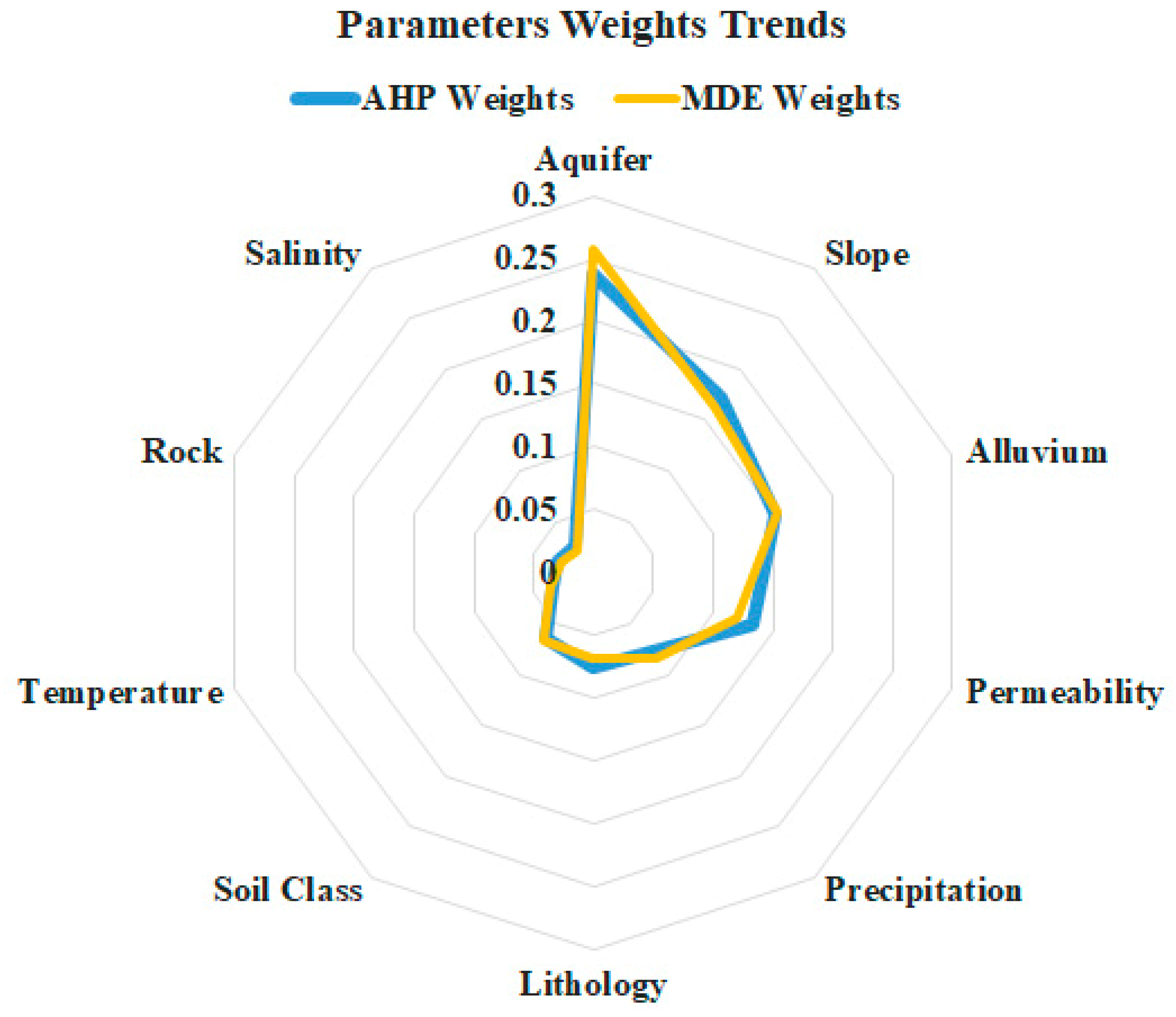
4.1. Finding the Weights of the Criteria with AHP
4.2. Finding Weights with Multi-Population-Based Differential Evolution Algorithm (MDE)
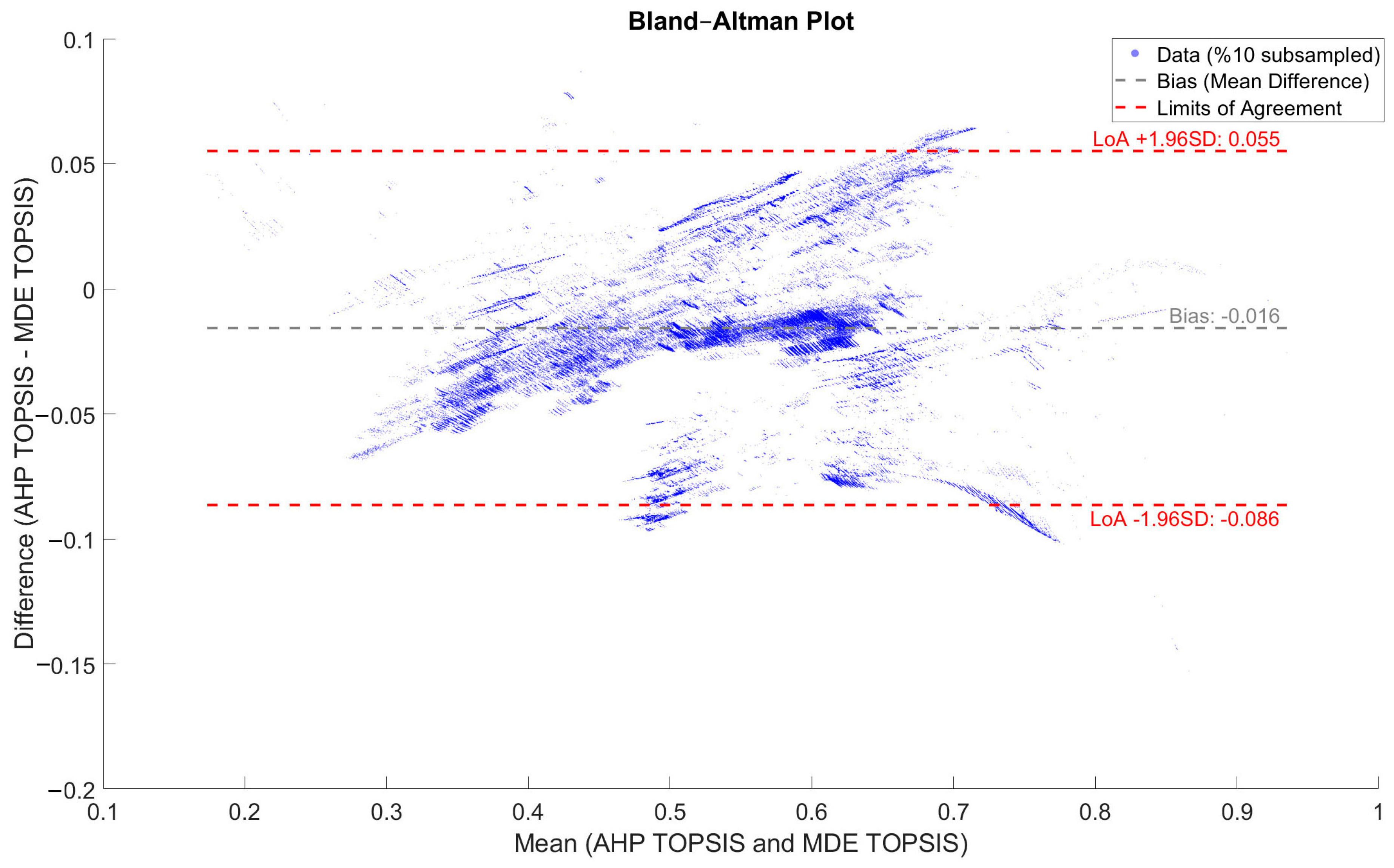
4.3. Ranking and Validation of Weights with TOPSIS
5. Discussion
6. Conclusions
Author Contributions
Funding
Institutional Review Board Statement
Data Availability Statement
Acknowledgments
Conflicts of Interest
References
- Başçiftçi, F.; Durduran, S.; İnal, C. Konya kapalı havzasında yeraltı su seviyelerinin coğrafi bilgi sistemi (CBS) ile haritalanması. Harit. Teknol. Elektron. Derg. 2013, 5, 1–15. [Google Scholar]
- Bingül, B.; Bengi, E.; Tutkal, Z.; Altunsoy, A.; Aksoy, T. TUCBS Veri standartları kullanılarak su kaynakları yönetimi değerlendirmesi. Balıkesir Üniversitesi Fen Bilim. Enstitüsü Derg. 2024, 26, 1–18. [Google Scholar] [CrossRef]
- Anh, D.T.; Pandey, M.; Mishra, V.N.; Singh, K.K.; Ahmadi, K.; Janizadeh, S.; Tran, T.T.; Linh, N.T.T.; Dang, N.M. Assessment of groundwater potential modeling using support vector machine optimization based on Bayesian multi-objective hyperparameter algorithm. Appl. Soft Comput. 2022, 132, 109848. [Google Scholar] [CrossRef]
- Khosravi, K.; Panahi, M.; Tien Bui, D. Spatial prediction of groundwater spring potential mapping based on an adaptive neuro-fuzzy inference system and metaheuristic optimization. Hydrol. Earth Syst. Sci. 2018, 22, 4771–4792. [Google Scholar] [CrossRef]
- Chen, W.; Panahi, M.; Khosravi, K.; Pourghasemi, H.R.; Rezaie, F.; Parvinnezhad, D. Spatial prediction of groundwater potentiality using ANFIS ensembled with teaching-learning-based and biogeography-based optimization. J. Hydrol. 2019, 572, 435–448. [Google Scholar] [CrossRef]
- Shiklomanov, I. Water in Crisis. In Water in Crisis: A Guide to World’s Freshwater Resources; Gleick, P.H., Ed.; Oxford University Press: New York, NY, USA, 1993; pp. 13–24. [Google Scholar]
- Gleick, P.H. Water Resources; Oxford University Press: New York, NY, USA, 1993; Volume 2, pp. 817–823. [Google Scholar]
- USGS. Where is Earth’s Water? Available online: https://www.usgs.gov/special-topics/water-science-school/science/where-earths-water (accessed on 1 March 2025).
- Rahmati, O.; Naghibi, S.A.; Shahabi, H.; Bui, D.T.; Pradhan, B.; Azareh, A.; Rafiei-Sardooi, E.; Samani, A.N.; Melesse, A.M. Groundwater spring potential modelling: Comprising the capability and robustness of three different modeling approaches. J. Hydrol. 2018, 565, 248–261. [Google Scholar] [CrossRef]
- Panahi, M.; Sadhasivam, N.; Pourghasemi, H.R.; Rezaie, F.; Lee, S. Spatial prediction of groundwater potential mapping based on convolutional neural network (CNN) and support vector regression (SVR). J. Hydrol. 2020, 588, 125033. [Google Scholar] [CrossRef]
- Bai, Z.; Liu, Q.; Liu, Y. Groundwater Potential Mapping in Hubei Region of China Using Machine Learning, Ensemble Learning, Deep Learning and AutoML Methods. Nat. Resour. Res. 2022, 31, 2549–2569. [Google Scholar] [CrossRef]
- Jia, Z.; Bian, J.; Wang, Y. Impacts of urban land use on the spatial distribution of groundwater pollution, Harbin City, Northeast China. J. Contam. Hydrol. 2018, 215, 29–38. [Google Scholar] [CrossRef]
- Oh, H.-J.; Kim, Y.-S.; Choi, J.-K.; Park, E.; Lee, S. GIS mapping of regional probabilistic groundwater potential in the area of Pohang City, Korea. J. Hydrol. 2011, 399, 158–172. [Google Scholar] [CrossRef]
- Jha, M.K.; Chowdary, V.M.; Chowdhury, A. Groundwater assessment in Salboni Block, West Bengal (India) using remote sensing, geographical information system and multi-criteria decision analysis techniques. Hydrogeol. J. 2010, 18, 1713–1728. [Google Scholar] [CrossRef]
- Arabameri, A.; Arora, A.; Pal, S.C.; Mitra, S.; Saha, A.; Nalivan, O.A.; Panahi, S.; Moayedi, H. K-Fold and State-of-the-Art Metaheuristic Machine Learning Approaches for Groundwater Potential Modelling. Water Resour. Manag. 2021, 35, 1837–1869. [Google Scholar] [CrossRef]
- Azma, A.; Narreie, E.; Shojaaddini, A.; Kianfar, N.; Kiyanfar, R.; Alizadeh, S.M.S.; Davarpanah, A. Statistical Modeling for Spatial Groundwater Potential Map Based on GIS Technique. Sustainability 2021, 13, 3788. [Google Scholar] [CrossRef]
- Pasupuleti, S.; Singha, S.S.; Kumar, S. Effectiveness of groundwater heavy metal pollution indices studies by deep-learning. J. Contam. Hydrol. 2020, 235, 103718. [Google Scholar] [CrossRef]
- Pradhan, A.M.S.; Kim, Y.-T.; Shrestha, S.; Huynh, T.-C.; Nguyen, B.-P. Application of deep neural network to capture groundwater potential zone in mountainous terrain, Nepal Himalaya. Environ. Sci. Pollut. Res. 2021, 28, 18501–18517. [Google Scholar] [CrossRef]
- Kaliraj, S.; Chandrasekar, N.; Magesh, N.S. Identification of potential groundwater recharge zones in Vaigai upper basin, Tamil Nadu, using GIS-based analytical hierarchical process (AHP) technique. Arab. J. Geosci. 2014, 7, 1385–1401. [Google Scholar] [CrossRef]
- Rahmati, O.; Samani, A.N.; Mahdavi, M.; Pourghasemi, H.R.; Zeinivand, H. Groundwater potential mapping at Kurdistan region of Iran using analytic hierarchy process and GIS. Arab. J. Geosci. 2015, 8, 7059–7071. [Google Scholar] [CrossRef]
- Shekhar, S.; Pandey, A.C. Delineation of groundwater potential zone in hard rock terrain of India using remote sensing, geographical information system (GIS) and analytic hierarchy process (AHP) techniques. Geocarto Int. 2015, 30, 402–421. [Google Scholar] [CrossRef]
- Pradhan, S.; Kumar, S.; Kumar, Y.; Sharma, H.C. Assessment of groundwater utilization status and prediction of water table depth using different heuristic models in an Indian interbasin. Soft Comput. 2019, 23, 10261–10285. [Google Scholar] [CrossRef]
- Siade, A.; Rathi, B.; Prommer, H.; Welter, D.; Doherty, J. Using heuristic multi-objective optimization for quantifying predictive uncertainty associated with groundwater flow and reactive transport models. J. Hydrol. 2019, 577, 123999. [Google Scholar] [CrossRef]
- Dehghani, R.; Poudeh, H.T.; Izadi, Z. The effect of climate change on groundwater level and its prediction using modern meta-heuristic model. Groundw. Sustain. Dev. 2022, 16, 100702. [Google Scholar] [CrossRef]
- Varouchakis, Ε.A.; Hristopulos, D.T. Comparison of stochastic and deterministic methods for mapping groundwater level spatial variability in sparsely monitored basins. Environ. Monit. Assess. 2013, 185, 1–19. [Google Scholar] [CrossRef] [PubMed]
- Fenta, A.A.; Kifle, A.; Gebreyohannes, T.; Hailu, G. Spatial analysis of groundwater potential using remote sensing and GIS-based multi-criteria evaluation in Raya Valley, northern Ethiopia. Hydrogeol. J. 2015, 23, 195–206. [Google Scholar] [CrossRef]
- Cerlini, P.B.; Silvestri, L.; Meniconi, S.; Brunone, B. Simulation of the Water Table Elevation in Shallow Unconfined Aquifers by means of the ERA5 Soil Moisture Dataset: The Umbria Region Case Study. Earth Interact. 2021, 25, 15–32. [Google Scholar] [CrossRef]
- Tamiru, H.; Wagari, M.; Tadese, B. An integrated Artificial Intelligence and GIS spatial analyst tools for Delineation of Groundwater Potential Zones in complex terrain: Fincha Catchment, Abay Basi, Ethiopia. Air Soil Water Res. 2022, 15, 45972. [Google Scholar] [CrossRef]
- Mozaffari, S.; Javadi, S.; Moghaddam, H.K.; Randhir, T.O. Forecasting Groundwater Levels using a Hybrid of Support Vector Regression and Particle Swarm Optimization. Water Resour. Manag. 2022, 36, 1955–1972. [Google Scholar] [CrossRef]
- Talebi, A.; Zahedi, E.; Hassan, M.A.; Lesani, M.T. Locating suitable sites for the construction of underground dams using the subsurface flow simulation (SWAT model) and analytical network process (ANP) (case study: Daroongar watershed, Iran). Sustain. Water Resour. Manag. 2019, 5, 1369–1378. [Google Scholar] [CrossRef]
- Baharvand, S.; Rahnamarad, J.; Soori, S. Assessment of the potential areas for underground dam construction in Roomeshgan, Lorestan province, Iran. Iran. J. Earth Sci. 2020, 12, 32–41. [Google Scholar]
- Kibar, H.; Kibar, B.; Sürmen, M. Sıcaklık ve yağış değişiminin Iğdır ilinde bitkisel ürün deseni üzerine etkileri. Adnan Menderes Üniversitesi Ziraat Fakültesi Derg. 2014, 11, 11–24. [Google Scholar]
- Altan, K.; Teksoy, A.; Solmaz, S.K.A. Türkiye’de yağış ve sıcaklığın su kaynakları, tarımsal ürün verimi ve su politikalarına etkisi. Uludağ Üniversitesi Mühendislik Fakültesi Derg. 2020, 25, 1253–1270. [Google Scholar]
- Malik, I.; Ahmed, M.; Gulzar, Y.; Baba, S.H.; Mir, M.S.; Soomro, A.B.; Sultan, A.; Elwasila, O. Estimation of the Extent of the Vulnerability of Agriculture to Climate Change Using Analytical and Deep-Learning Methods: A Case Study in Jammu, Kashmir, and Ladakh. Sustainability 2023, 15, 11465. [Google Scholar] [CrossRef]
- Abuelaish, B.S.; Olmedo, M.T.C. Analysis and Modelling of Groundwater Salinity Dynamics in the Gaza strip. Cuad. Geogr. Univ. Granada 2018, 57, 72–91. [Google Scholar] [CrossRef]
- Mosavi, A.; Hosseini, F.S.; Choubin, B.; Taromideh, F.; Ghodsi, M.; Nazari, B.; Dineva, A.A. Susceptibility mapping of groundwater salinity using machine learning models. Environ. Sci. Pollut. Res. 2021, 28, 10804–10817. [Google Scholar] [CrossRef] [PubMed]
- Kharazi, P.; Yazdani, M.R.; Khazealpour, P. Suitable identification of underground dam locations, using decision-making methods in a semi-arid region of Iranian Semnan Plain. Groundw. Sustain. Dev. 2019, 9, 100240. [Google Scholar] [CrossRef]
- Sun, Y.; Kang, S.; Li, F.; Zhang, L. Comparison of interpolation methods for depth to groundwater and its temporal and spatial variations in the Minqin oasis of northwest China. Environ. Model. Softw. 2009, 24, 1163–1170. [Google Scholar] [CrossRef]
- Arkoç, O. Trakya Bölgesi, Hayrabolu havzasında akiferin kirlenmeye karşı duyarlılığının DRASTIC ve DRASTIC-AHP yöntemleri ile haritalanması. Kafkas Üniversitesi Fen Bilim. Enstitüsü Derg. 2018, 11, 6–22. [Google Scholar]
- Aslan, V. Bozova Groundwater Quality Modeling and Evaluation Using Fuzzy Ahp Method Based on Gıs Technique. J. Anatol. Environ. Anim. Sci. 2023, 8, 16–27. [Google Scholar] [CrossRef]
- Saaty, T.L. Decision making for leaders. IEEE Trans. Syst. Man Cybern. 1985, SMC-15, 450–452. [Google Scholar] [CrossRef]
- Ünal, Z. Analitik hiyerarşi yöntemi ile bitki koruma makinesi seçimi: Mısır bitkisi örneği. Turk. J. Agric.-Food Sci. Technol. 2024, 12, 453–461. [Google Scholar] [CrossRef]
- Saaty, T.L. The analytic hierarchy process (AHP). J. Oper. Res. Soc. 1980, 41, 1073–1076. [Google Scholar]
- Sales, A.C.M.; Guimarães, L.G.d.A.; Neto, A.R.V.; El-Aouar, W.A.; Pereira, G.R. Risk assessment model in inventory management using the AHP method. Gestão Produção 2020, 27, e4537. [Google Scholar] [CrossRef]
- Saaty, T.L.; Vargas, L.G. The Logic of Priorities; Springer: Berlin/Heidelberg, Germany, 1982. [Google Scholar]
- Hwang, C.-L.; Yoon, K.; Hwang, C.-L.; Yoon, K. Methods for multiple attribute decision making. In Multiple Attribute Decision Making: Methods and Applications a State-of-the-Art Survey; Springer: Berlin/Heidelberg, Germany, 1981; pp. 58–191. [Google Scholar]
- Ünal, Z.; Çetin, E.İ. Gübre üreticisinin hedef pazar seçiminde bütünleşik AHP-TOPSIS yöntemi. Mediterr. Agric. Sci. 2019, 32, 357–364. [Google Scholar] [CrossRef]
- Civicioglu, P.; Besdok, E. Colony-Based Search Algorithm for numerical optimization. Appl. Soft Comput. 2023, 151, 111162. [Google Scholar] [CrossRef]
- Holland, J. Adaptation in Artificial and Natural Systems; The University of Michigan Press: Ann Arbor, MI, USA, 1975; p. 232. [Google Scholar]
- Storn, R.; Price, K. Differential evolution—A simple and efficient heuristic for global optimization over continuous spaces. J. Glob. Optim. 1997, 11, 341–359. [Google Scholar] [CrossRef]
- Dorigo, M.; Birattari, M.; Stutzle, T. Ant colony optimization. IEEE Comput. Intell. Mag. 2007, 1, 28–39. [Google Scholar] [CrossRef]
- Kennedy, J.; Eberhart, R. Particle swarm optimization. In Proceedings of the ICNN’95 International Conference on Neural Networks, Perth, WA, Australia, 27 November–1 December 1995; pp. 1942–1948. [Google Scholar]
- Karaboga, D.; Basturk, B. A powerful and efficient algorithm for numerical function optimization: Artificial bee colony (ABC) algorithm. J. Glob. Optim. 2007, 39, 459–471. [Google Scholar] [CrossRef]
- Karkinli, A.E. Detection of object boundary from point cloud by using multi-population based differential evolution algorithm. Neural Comput. Appl. 2022, 35, 5193–5206. [Google Scholar] [CrossRef]
- Hüsrevoğlu, M.; Karkınlı, A.E. Enhanced Pansharpening Using Curvelet Transform Optimized by Multi Population Based Differential Evolution. Int. J. Sci. Res. Comput. Sci. Eng. Inf. Technol. 2024, 10, 139–149. [Google Scholar] [CrossRef]
- Mandal, T.; Saha, S.; Das, J.; Sarkar, A. Groundwater depletion susceptibility zonation using TOPSIS model in Bhagirathi river basin, India. Model. Earth Syst. Environ. 2021, 8, 1711–1731. [Google Scholar] [CrossRef]
- Li, Q.; Sui, W.; Sun, B.; Li, D.; Yu, S. Application of TOPSIS water abundance comprehensive evaluation method for karst aquifers in a lead zinc mine, China. Earth Sci. Inform. 2022, 15, 397–411. [Google Scholar] [CrossRef]
- Barman, J.; Biswas, B. Application of e-TOPSIS for Ground Water Potentiality Zonation using Morphometric Parameters and Geospatial Technology of Vanvate Lui Basin, Mizoram, NE India. J. Geol. Soc. India 2022, 98, 1385–1394. [Google Scholar] [CrossRef]
- Patidar, N.; Mohseni, U.; Pathan, A.I.; Agnihotri, P.G. Groundwater Potential Zone Mapping Using an Integrated Approach of GIS-Based AHP-TOPSIS in Ujjain District, Madhya Pradesh, India. Water Conserv. Sci. Eng. 2022, 7, 267–282. [Google Scholar] [CrossRef]
- Paul, S.; Roy, D. Geospatial modeling and analysis of groundwater stress-prone areas using GIS-based TOPSIS, VIKOR, and EDAS techniques in Murshidabad district, India. Model. Earth Syst. Environ. 2024, 10, 121–141. [Google Scholar] [CrossRef]
- Rahimabadi, P.D.; Behnia, M.; Molaei, S.N.; Khosravi, H.; Azarnivand, H. Assessment of groundwater resources potential using Improved Water Quality Index (ImpWQI) and entropy-weighted TOPSIS model. Sustain. Water Resour. Manag. 2024, 10, 1–13. [Google Scholar] [CrossRef]
- Elumalai, V.; Brindha, K.; Sithole, B.; Lakshmanan, E. Spatial interpolation methods and geostatistics for mapping groundwater contamination in a coastal area. Environ. Sci. Pollut. Res. 2017, 24, 11601–11617. [Google Scholar] [CrossRef]
- Ghosh, M.; Pal, D.K.; Santra, S.C. Spatial mapping and modeling of arsenic contamination of groundwater and risk assessment through geospatial interpolation technique. Environ. Dev. Sustain. 2020, 22, 2861–2880. [Google Scholar] [CrossRef]
- Rizeei, H.M.; Pradhan, B.; Saharkhiz, M.A.; Lee, S. Groundwater aquifer potential modeling using an ensemble multi-adoptive boosting logistic regression technique. J. Hydrol. 2019, 579, 124172. [Google Scholar] [CrossRef]
- El Ayady, H.; Mickus, K.L.; Boutaleb, S.; Morjani, Z.E.A.E.; Ikirri, M.; Echogdali, F.Z.; Bessa, A.Z.E.; Abdelrahman, K.; Id-Belqas, M.; Essoussi, S.; et al. Investigation of groundwater potential using geomatics and geophysical methods: Case study of the Anzi sub-basin, western Anti-Atlas, Morocco. Adv. Space Res. 2023, 72, 3960–3981. [Google Scholar] [CrossRef]
- Fawcett, T. An introduction to ROC analysis. Pattern Recognit. Lett. 2006, 27, 861–874. [Google Scholar] [CrossRef]
- Metz, C.E. Basic principles of ROC analysis. Semin. Nucl. Med. 1978, 8, 283–298. [Google Scholar] [CrossRef]
- Pourghasemi, H.R.; Pradhan, B.; Gokceoglu, C. Application of fuzzy logic and analytical hierarchy process (AHP) to landslide susceptibility mapping at Haraz watershed, Iran. Nat. Hazards 2012, 63, 965–996. [Google Scholar] [CrossRef]
- Arulbalaji, P.; Padmalal, D.; Sreelash, K. GIS and AHP Techniques Based Delineation of Groundwater Potential Zones: A case study from Southern Western Ghats, India. Sci. Rep. 2019, 9, 2082. [Google Scholar] [CrossRef] [PubMed]
- Achu, A.L.; Thomas, J.; Reghunath, R. Multi-criteria decision analysis for delineation of groundwater potential zones in a tropical river basin using remote sensing, GIS and analytical hierarchy process (AHP). Groundw. Sustain. Dev. 2020, 10, 100365. [Google Scholar] [CrossRef]
- Kaur, L.; Rishi, M.S.; Singh, G.; Thakur, S.N. Groundwater potential assessment of an alluvial aquifer in Yamuna sub-basin (Panipat region) using remote sensing and GIS techniques in conjunction with analytical hierarchy process (AHP) and catastrophe theory (CT). Ecol. Indic. 2020, 110, 105850. [Google Scholar] [CrossRef]
- Aykut, T. Determination of groundwater potential zones using Geographical Information Systems (GIS) and Analytic Hierarchy Process (AHP) between Edirne-Kalkansogut (northwestern Turkey). Groundw. Sustain. Dev. 2021, 12, 100545. [Google Scholar] [CrossRef]
- Gumma, M.K.; Pavelic, P. Mapping of groundwater potential zones across Ghana using remote sensing, geographic information systems, and spatial modeling. Environ. Monit. Assess. 2013, 185, 3561–3579. [Google Scholar] [CrossRef]
- Kumar, R.; Dwivedi, S.B.; Gaur, S. A comparative study of machine learning and Fuzzy-AHP technique to groundwater potential mapping in the data-scarce region. Comput. Geosci. 2021, 155, 104855. [Google Scholar] [CrossRef]
- Ardakani, A.H.H.; Shojaei, S.; Siasar, H.; Ekhtesasi, M.R. Heuristic Evaluation of Groundwater in Arid Zones Using Remote Sensing and Geographic Information System. Int. J. Environ. Sci. Technol. 2020, 17, 633–644. [Google Scholar] [CrossRef]


| Reference | Criteria | Method | Study Area |
|---|---|---|---|
| [13] | Groundwater productivity and hydrogeological factors, such as land cover, topology, geology, groundwater table distribution, and groundwater recharge | GIS | Pohang, Korea |
| [25] | Hydrogeological data | It compares the interpolation performance of kriging, universal kriging, and Delaunay triangulation with IDW and minimum curvature (MC) deterministic methods | Mires Basin of Mesara Valley in Crete (Greece) |
| [26] | Lithology, lineament density, geomorphology, slope, drainage density, rainfall, and land use/cover | GIS, remote sensing, and multi-criteria decision-making techniques | Raya Valley in northern Ethiopia |
| [4] | Slope degree, slope aspect, altitude plan curvature, topographic wetness index (TWI), terrain roughness index (TRI), distance from fault, distance from river, land use/land cover, rainfall soil order, geology (unit) | Neuro-fuzzy inference system (ANFIS), invasive weed optimization (IWO), differential evolution, (DE), firefly algorithm (FA), particle swarm optimization (PSO), and bee algorithm (BA) | Koohdasht-Nourabad plain, Lorestan province, Iran |
| [5] | Slope direction, altitude, slope angle, plan curvature, profile curvature, curvature, sediment transport index, stream power index, topographic wetness index, distance to roads, distance to rivers, rainfall, lithology, soil as input variables, Landsat normalized difference vegetation index (NDVI), and land use/land cover | Teaching, learning-based optimization, and two new hybrid data-mining techniques, including adaptive biogeography fused with biogeography (ANFIS) | Zhangjiamao in China |
| [10] | Catchment area, convergence index, convexity, diurnal anisotropic heating, flow path, slope angle, slope height, topographic position index, terrain ruggedness index, slope length factor, mass balance index, texture, valley depth, land cover, and geology | Comparison of the predictive capabilities of support vector regression (SVR) and convolutional neural networks (CNNs) in groundwater potential mapping | South Korea, Damyang area |
| [15] | Elevation, slope, curvature, aspect, drainage density, fault density, distance from the stream, distance from fault, terrain surface texture (TST), (TRI), height above nearest drainage (HAND), rainfall, lithology, and land use | An approach that combines the implementation of four scenarios, each involving ANFIS with six machine learning models | Lake Urmia Basin in northwestern Iran |
| [16] | Elevation, TWI, slope, aspect, soil clay, soil electrical conductivity (SEC), groundwater EC (GEC) | GIS-based statistical mapping | Iran |
| [27] | Water table elevation measurements and soil moisture at different depths (ERA5 reanalysis dataset) | Proposed method for simulating water table elevation in shallow unconfined aquifers using soil moisture time series and piezometer measurements | Umbria region of Italy |
| [28] | Rainfall, land use/land cover, drainage density, lineament density, slope, geology, soil, geomorphology | Artificial neural networks, analytical hierarchy process, GIS | Abay, Ethiopia, Fincha Basin |
| [29] | Aquifer | A simulation–optimization hybrid model was developed. The model uses SVM to predict groundwater levels and the particle swarm optimization algorithm and Bayesian network to optimize its parameters. | Zanjan aquifer in Iran |
| [11] | Slope, elevation, curvature, landforms, geology, distance to faults, land type, soils, precipitation, evaporation, TWI, stream power index (SPI), distance to rivers, NDVI, and distance to residential area. | Machine learning, ensemble learning, deep learning, and automated machine learning | Hubei Province of China |
| [3] | Elevation, aspect, slope, plan curvature, profile curvature, distance from the fault, distance from the road, distance from the river, drainage density, land use, lithology, soil, SPI, TWI, annual precipitation, precipitation of coldest month, precipitation of coldest season, precipitation of wettest month. | Multivariate adaptive regression splines algorithm and support vector regression machine learning models were used. Comparison of prediction capabilities using random search and Bayesian optimization hyperparameter algorithm to optimize the parameters of the SVM model | Markazi Province of Iran |
| This Study | Aquifer, slope, permeability alluvial soils, soil quality lithology, temperature and precipitation salinity, stone density | GIS, AHP, TOPSIS, and heuristic methods | Beyşehir and Çumra sub-basins of Konya Province, Turkey |
| Study Area | Criteria and Sub-Criteria | Production of Maps | Resources |
|---|---|---|---|
| Beysehir and Cumra sub-basins | Aquifer | The map is produced by interpolation according to the aquifer-specific productivity values obtained from the reports provided by State Water Affairs. | State Water Affairs |
| Slope | Slope analysis is performed and a map is produced by classifying it according to a 2% slope change. | Minister of Environment, Urbanisation, and Climate Change | |
| Permeability | Permeability is scored by experts according to the structure of the ground and the suitability of water availability. The map is produced according to this scoring. | State Water Affairs | |
| Alluvial soils | The availability of groundwater increases depending on the thickness of the alluvium. The map is produced by interpolating the alluvial thicknesses from the reports provided by the Minister of Environment, Urbanisation, and Climate Change | Minister of Environment, Urbanisation, and Climate Change | |
| Soil Quality | Soil classes are scored by experts according to their suitability for groundwater presence. The map is produced according to this scoring. | State Water Affairs | |
| Lithology | There are 16 lithology layers in the studied basin area. Each lithology layer is scored by experts according to its suitability for groundwater presence. The map is produced according to this scoring. | Mineral Research and Exploration General Directorate | |
| Precipitation | A rainfall map is produced by interpolating the cumulative sum of rainfall in the last five years (2019–2023). | Meteorological Service | |
| Temperature | A temperature map is produced by interpolating the cumulative sum of the temperature in the last five years (2019–2023). | Meteorological Service | |
| Salinity | The map is produced by eliminating salt domes and sediment areas. | Minister of Environment, Urbanisation, and Climate Change | |
| Stone Density | Stone impact and stone density are scored by experts according to their suitability for groundwater presence. The map is produced according to this scoring. | State Water Affairs |
| Aq | Slp | Per | AS | SQ | Lit | Pr | Tmp | Sal | SD | |
|---|---|---|---|---|---|---|---|---|---|---|
| Aq | 1.00 | 2.85 | 1.95 | 1.38 | 5.84 | 3.77 | 2.62 | 5.33 | 6.56 | 5.84 |
| Slp | 0.35 | 1.00 | 2.13 | 1.05 | 4.68 | 2.80 | 2.36 | 4.44 | 6.03 | 5.76 |
| Per | 0.51 | 0.47 | 1.00 | 1.05 | 4.33 | 2.04 | 2.04 | 3.60 | 4.74 | 4.16 |
| AS | 0.73 | 0.96 | 0.96 | 1.00 | 4.47 | 2.47 | 1.95 | 4.50 | 5.16 | 3.56 |
| SQ | 0.17 | 0.21 | 0.23 | 0.22 | 1.00 | 1.43 | 2.16 | 1.80 | 3.49 | 1.94 |
| Lit | 0.27 | 0.36 | 0.49 | 0.40 | 0.70 | 1.00 | 1.73 | 2.81 | 4.47 | 2.27 |
| Pr | 0.38 | 0.42 | 0.49 | 0.51 | 0.46 | 0.58 | 1.00 | 3.65 | 4.35 | 2.96 |
| Tmp | 0.19 | 0.23 | 0.28 | 0.22 | 0.56 | 0.36 | 0.27 | 1.00 | 1.65 | 1.29 |
| Sal | 0.15 | 0.17 | 0.21 | 0.19 | 0.29 | 0.22 | 0.23 | 0.61 | 1.00 | 1.04 |
| SD | 0.17 | 0.17 | 0.24 | 0.28 | 0.51 | 0.44 | 0.34 | 0.78 | 0.96 | 1.00 |
| Aq | Slp | Per | AS | SQ | Lit | Pr | Tmp | Sal | SD | |
|---|---|---|---|---|---|---|---|---|---|---|
| Aq | 0.26 | 0.42 | 0.25 | 0.22 | 0.26 | 0.25 | 0.18 | 0.19 | 0.17 | 0.20 |
| Slp | 0.09 | 0.15 | 0.27 | 0.17 | 0.20 | 0.19 | 0.16 | 0.16 | 0.16 | 0.19 |
| Per | 0.13 | 0.07 | 0.13 | 0.17 | 0.19 | 0.14 | 0.14 | 0.13 | 0.12 | 0.14 |
| AS | 0.19 | 0.14 | 0.12 | 0.16 | 0.20 | 0.16 | 0.13 | 0.16 | 0.13 | 0.12 |
| SQ | 0.04 | 0.03 | 0.03 | 0.04 | 0.04 | 0.09 | 0.15 | 0.06 | 0.09 | 0.07 |
| Lit | 0.07 | 0.05 | 0.06 | 0.06 | 0.03 | 0.07 | 0.12 | 0.10 | 0.12 | 0.08 |
| Pr | 0.10 | 0.06 | 0.06 | 0.08 | 0.02 | 0.04 | 0.07 | 0.13 | 0.11 | 0.10 |
| Tmp | 0.05 | 0.03 | 0.03 | 0.04 | 0.02 | 0.02 | 0.02 | 0.04 | 0.04 | 0.04 |
| Sal | 0.04 | 0.02 | 0.03 | 0.03 | 0.01 | 0.01 | 0.02 | 0.02 | 0.03 | 0.03 |
| SD | 0.04 | 0.03 | 0.03 | 0.04 | 0.02 | 0.03 | 0.02 | 0.03 | 0.03 | 0.03 |
| Criterion | Weights |
|---|---|
| Aquifer | 0.237 |
| Slope | 0.172 |
| Alluvial Soils | 0.151 |
| Permeability | 0.134 |
| Precipitation | 0.077 |
| Lithology | 0.075 |
| Soil Quality | 0.064 |
| Temperature | 0.034 |
| Stone Density | 0.031 |
| Salinity | 0.025 |
| Criterion | MDE |
|---|---|
| Aquifer | 0.258 |
| Alluvial Soils | 0.164 |
| Slope | 0.153 |
| Permeability | 0.119 |
| Precipitation | 0.084 |
| Soil Quality | 0.069 |
| Lithology | 0.067 |
| Temperature | 0.037 |
| Stone Density | 0.027 |
| Salinity | 0.022 |
| Model 1 | Model 2 | |
|---|---|---|
| AHP and TOPSIS | MDE and TOPSIS | |
| RMSE | 114.219 | 114.209 |
| MSE | 13,046.091 | 13,043.785 |
| MAE | 99.663 | 99.652 |
Disclaimer/Publisher’s Note: The statements, opinions and data contained in all publications are solely those of the individual author(s) and contributor(s) and not of MDPI and/or the editor(s). MDPI and/or the editor(s) disclaim responsibility for any injury to people or property resulting from any ideas, methods, instructions or products referred to in the content. |
© 2025 by the authors. Licensee MDPI, Basel, Switzerland. This article is an open access article distributed under the terms and conditions of the Creative Commons Attribution (CC BY) license (https://creativecommons.org/licenses/by/4.0/).
Share and Cite
Bozdağ, A.; Ünal, Z.; Karkınlı, A.E.; Soomro, A.B.; Mir, M.S.; Gulzar, Y. An Integrated Approach for Groundwater Potential Prediction Using Multi-Criteria and Heuristic Methods. Water 2025, 17, 1212. https://doi.org/10.3390/w17081212
Bozdağ A, Ünal Z, Karkınlı AE, Soomro AB, Mir MS, Gulzar Y. An Integrated Approach for Groundwater Potential Prediction Using Multi-Criteria and Heuristic Methods. Water. 2025; 17(8):1212. https://doi.org/10.3390/w17081212
Chicago/Turabian StyleBozdağ, Aslı, Zeynep Ünal, Ahmet Emin Karkınlı, Arjumand Bano Soomro, Mohammad Shuaib Mir, and Yonis Gulzar. 2025. "An Integrated Approach for Groundwater Potential Prediction Using Multi-Criteria and Heuristic Methods" Water 17, no. 8: 1212. https://doi.org/10.3390/w17081212
APA StyleBozdağ, A., Ünal, Z., Karkınlı, A. E., Soomro, A. B., Mir, M. S., & Gulzar, Y. (2025). An Integrated Approach for Groundwater Potential Prediction Using Multi-Criteria and Heuristic Methods. Water, 17(8), 1212. https://doi.org/10.3390/w17081212