Water-Quality Spatiotemporal Characteristics and Their Drivers for Two Urban Streams in Indianapolis

Abstract

Water quality in urban streams is critical for the health of aquatic and human life, as it impacts both the environment and water availability. The strong impacts of changing climate and land use on water quality necessitate a better understanding of how stream water quality changes over space and time. To this end, four key water-quality parameters—Escherichia coli (E. coli), nitrate (NO₃⁻), sulfate (SO₄²⁻), and chloride (Cl⁻)—were collected at 12 sites along Fall Creek and Pleasant Run streams in Indianapolis, Indiana USA from 2003 to 2021 on a seasonal basis: March, July, and October each year. Two-way ANOVA tests were used to determine the impacts of seasonality and location on these parameters. Correlation and RDA (redundancy analysis) were used to determine the importance of climatic drivers. Linear regressions were used to quantify the impacts of land-use types on water quality integrating buffer zone size and sub-watershed analysis. Strong seasonal variations of the water-quality parameters were found. March had higher levels of NO₃⁻, SO₄²⁻, and Cl⁻ than other months. July had the highest E. coli concentrations compared to March and October. Seven-days antecedent snow and precipitation were found to be significantly related to Cl⁻ and log₁₀(E. coli) and can explain up to 53% and 31% of their variations, respectively. Spatially, urban built-up land in a 1000 m buffer around the sampling sites was positively correlated with the log₁₀(E. coli) variation, while lawn cover was positively related to NO₃⁻ concentrations within 500 m buffers. Conversely, NDVI (Normalized Difference Vegetation Index) values were negatively related to all variables. In conclusion, E. coli is more impacted by higher precipitation and urban land coverage, which could be related to more combined sewer overflow events in July. Cl⁻ peaking in March and its relationship with snow indicate salt runoff during snow melting events. NO₃⁻ and SO₄²⁻ increases are likely due to fertilizer input from residential lawns near streams. This suggests that Indianapolis stream water-quality changes are influenced by both changing climate and land-cover/-muse types.

1. Introduction

Water quality is important in urban ecology as it is associated with stormwater pollution, changing climate, and land-use changes. Urban waterways benefit society and ecosystems by providing clean drinking water and safe recreational water for urban populations, and they also provide a healthy habitat for aquatic life. However, urban water bears the burden of significant pollution from diverse sources such as industrial emissions, mobile sources (e.g., car and trucks), wastewater from residential and commercial areas, trash from sewer systems, and storm runoff from impervious surfaces [1]. A better understanding of spatial and temporal variations in urban water quality can increase access to clean water, sustain the health of city dwellers, and support water-related policies.

Human-induced climate change and land-use change exert a significant influence on urban water quality [2]. Changing climate has increased the frequency and intensity of extreme precipitation events, which can cause changes in urban streamflow and the release of excess pollutants from land to water [3]. Potential temperature shifts would affect chemical reactions and water circulation, thereby connecting with precipitation patterns to affect the streamflow dynamics and the transportation and dilution of contaminants, altering the concentration of pollutants and chemical fluxes in streams [4]. Urban land use introduces a series of pollutants from human activities to water bodies, including sewer contaminants, residues from street solids, road salts, and excessive lawn/garden fertilizers. Concurrently, urban expansion has increased land imperviousness and reduced the capacity for infiltration, resulting in more runoff from urban surface areas during heavy rainfall/snow events [2]. This increased urban runoff pressured by a changing climate carries pollutants into nearby urban waterways. Pollutants have a profound influence on stream chemistry and nutrient balances, which in turn can impair water quality and stream biota [5]. Despite being significant determinants of water quality, few studies have characterized the integrated impacts of changing climate and land use. Therefore, to enhance water resource conservation and better understand water-, land-, and climate-related problems, it is necessary to clarify the relationships between changing climate, human land-use change, and urban water qualities.

Escherichia coli (E. coli), chloride (Cl⁻), nitrate (NO₃⁻), and sulfate (SO₄²⁻) are typical water contaminants that are indicators of sewage, road salt, lawn fertilizer, and pose threats to humans and the environment. A higher concentration of E. coli may lead to bacterial infections, higher chloride concentration may lead to rising salinity in freshwater, and NO₃⁻ and SO₄²⁻ may accelerate eutrophication. The pollutant sources differ depending on different land-use practices, such as fertilizing the gardens and lawns or applying road salt on the streets in the winter. For example, a lawn appears to have high nitrate concentration, while streets have higher solids and higher chloride concentration in the winter [6,7]. In addition, residential areas contain higher toxic trace metal content than commercial surfaces [8,9], and industrial activities may result in an increase in sulfate concentration along the urban streamflow [10]. These findings suggested that the source(s) of pollutants has high spatial variability, and it needs to be identified based on diverse urban land to address the vulnerability of water infrastructure and the severity of water pollution.

Most older cities in the US have an old infrastructure system that delivers the combined sewer overflows and stormwater pollutants to local rivers. These pollutants originate from a variety of land-use practices and human activities, with their impact being frequent during wet weather. However, the conditions and drivers of water quality have not been clear in urban systems. To fill this gap, we investigated the urban water-quality issue using two urban streams of different sizes. The aims of this study are (1) to assess long-term and seasonal water-quality variations (E. coli/nitrate/sulfate/chloride) in two watersheds in the city of Indianapolis from 2003 to 2021; (2) to examine the spatial trends of water-quality variables along the streams; (3) to examine the water-quality variability that can be explained by changing climate factors (e.g., precipitation, temperature, snow) and land-use factors (e.g., urban built-up cover, lawn/tree cover, residential/industry land use) in varying spatial extents around sampling locations.

2. Materials and Methods

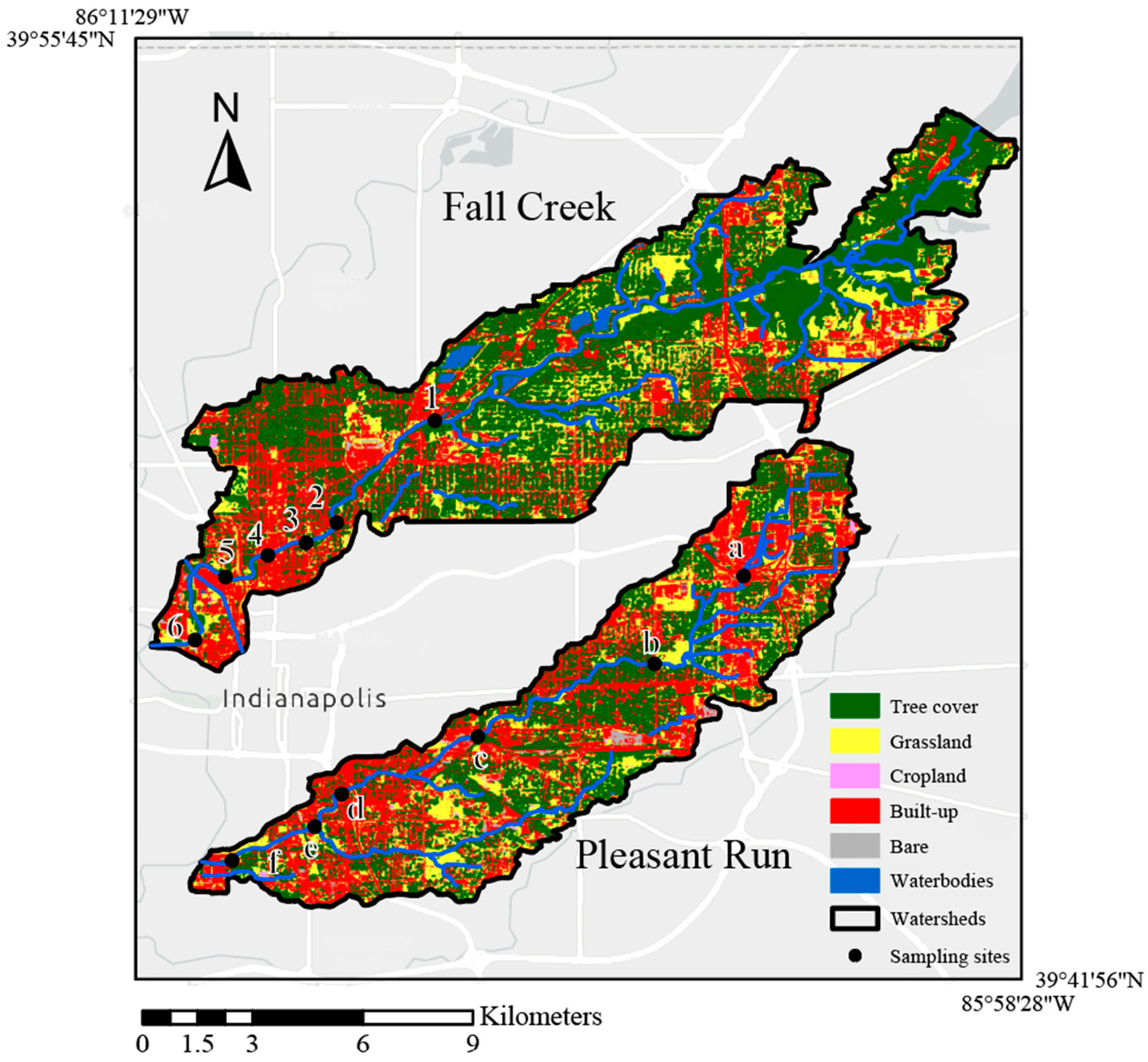
2.1. Study Area

Indianapolis is a midwestern U.S. city. It is in the Tipton Till Plain, a region defined by its mostly flat-to-gently rolling landscape formed by glacial products (Figure S1). The city is well known for its limestone and productive agricultural soil. The land gently slopes towards White River, which flows through the city and provides a significant water resource. Lots of streams feed the white river, including Fall Creek and Pleasant Run (Figure S2), shaping the city’s drainage system. Lots of streams feed the white river, including Fall Creek and Pleasant Run (Figure S1), shaping the city’s drainage system.

Pleasant Run and Fall Creek are two urban waterways in Indianapolis. They begin north of the city, flow towards the southwest, and run through several communities before merging into the White River (Figure 1). The mean annual temperature, precipitation, and snowfall from 2003 to 2021 in the area are around 12.2 °C, 1159 mm, and 635 mm, respectively (data from National Weather Service: https://www.weather.gov/wrh/climate?wfo=ind (accessed on 1 June 2022)). Fall Creek drains a watershed area of 107 km², while Pleasant Run drains 70 km². The two watersheds differ significantly in terms of their stream discharges, with Fall Creek exhibiting up to 10 times higher stream discharge than Pleasant Run (Data from USGS: U.S. Geological Survey). Despite the differences in hydrological characteristics, both watersheds mainly comprise urbanized areas (Figure 1). Due to urbanization and the relatively high annual precipitation, the two watersheds are particularly vulnerable to stormwater pollution. This includes various pollutants such as E. coli, lawn fertilizer, and road deicing salt. Additionally, stormwater pollution problems are projected to worsen as climate change is expected to cause more extreme rainfall events in the region. The city of Indianapolis aims to enhance stormwater management by constructing a deep tunnel system to divert stormwater from the sewer system to the deep tunnel for temporary storage and controlled release. The completion of the deep tunnel by 2025 will be a significant intervention in the stormwater pollution situation, as it is projected to reduce 90% of the pollutants entering urban waterways during rainfall events (https://info.citizensenergygroup.com/digindy (accessed on 1 June 2022)). Our study would allow a future comparison of water-quality conditions before and after the tunnel infrastructure upgrade.

2.2. Sampling and Measurement

Water samples were collected at 12 sites along the Fall Creek and Pleasant Run (Figure 1) by Marion County Health Department (MCHD, https://marionhealth.org/ (accessed on 1 March 2022)) from 2003 to 2021 on a seasonal basis: March, July, and October each year. Two-hundred-milliliter bottles were used for every water sample taken. Water temperature, pH, total dissolved solids (TDS, g/L), and dissolved oxygen (DO, mg/L) were determined on site by a Hydrolab Surveyor between 2003 and 2011 and a YSI Pro-Plus between 2012 and 2021. In the MCHD lab, four key parameters, E. coli, NO₃⁻, SO₄²⁻, and Cl⁻ concentrations, were measured, where E. coli (MPN/100 mL) was measured on the 1:10 dilution step by the Colilert test kits (IDEXX, US). NO₃⁻ (mg/L), SO₄²⁻ (mg/L), and Cl⁻ (mg/L) concentrations were determined by ion chromatography using the EPA (Environmental Protection Agency) method 300.0 [11]. E. coli test started the same day or the next day at the latest for the sampling routes. The other ions were tested at the end of the sampling routes each month.

2.3. Land-Cover Use and NDVI Data Preprocessing

To examine the association of land cover and land use on water quality, land-cover/use data were collected from various sources and summarized in circular buffers at multiple radii. The land-cover data were sourced from the 10 m resolution image of European Space Agency (ESA) World Cover 2021 [12]. In the image, urban built-up, tree cover, and grassland areas were summarized in 500 and 1000 m circular buffers around sampling locations. Land-use data from the Indy gov portal were calculated in 100 m, 250 m, 500 m, and 1000 m buffer sizes for comparing residential, industrial, parking lot, and street length association. Land-use data are from indy gov portal and parking lot data are from data.indy.gov/datasets/parking-lot-3/explore (accessed on 1 July 2022). Street data are from data.indy.gov/datasets/street-centerlines/explore (accessed on 1 July 2022). All land-cover data were preprocessed in Google Earth Engine (GEE). Land-use data were processed in ArcGIS Pro 3.2.1 and exported as Excel sheet data into Jupyter notebook for statistical analysis. The watershed tool in ArcGIS Pro was used to examine the sub-watershed area upstream of the sampling locations based on methods [13].

To assess the impact of vegetation on water-quality parameters in city streams, this study utilized the NDVI, which has been extensively used to monitor vegetation greenness and productivity [14,15,16] and to represent vegetation dynamics across water-sampling sites. The NDVI was derived from the daily nadir bidirectional reflectance distribution function (BRDF) adjusted reflectance product from Moderate-Resolution Imaging Spectroradiometer (MCD43A4 V006, 500 m) covering the period of water sampling. A 1000 m buffer was set up for each water sampling location to calculate the regional average NDVI. The NDVI data preprocessing was performed in GEE. The corresponding NDVI data matching the water sampling dates were used in the analysis.

2.4. Statistical Analyses

E. coli values were log-transformed to meet data normalization requirements for the statistical analyses. Log₁₀(E. coli), NO₃⁻, SO₄²⁻, and Cl⁻ concentrations were statistically analyzed over 19 years, among sampling months, and between two watersheds and 12 monitoring sites, respectively. To detect the time-series trends, the Mann–Kendall test was used to determine long-term trends of four parameters. Two-way ANOVA (Analysis of variance) tests and Tukey post-hoc tests were used to estimate which of the combinations of three sampling months and two watersheds are statistically different from one another for the four water-quality parameters. One-way ANOVA was used to determine spatial differences in water-quality parameters among 12 sites. To analyze potential climatic and environmental factors influencing the temporal dynamics, Spearman correlation and hierarchical clustering were conducted to analyze the relationships between water-quality parameters and environmental factors. Redundancy analysis (RDA) with forward selection was used to determine main contributors of explanatory drivers [17]. To identify land impacts, linear regression was applied to examine all associations between land-cover, land-use, NDVI, and water-quality factors.

All statistical analyses were performed in R software (R-4.1.1, R Core Team, 2022) and Jupyter notebook [18]. The Kendall and Vegan packages were used for M-K test. The ano() and TukeyHSD() functions were used for one-way and two-way ANOVA analysis and pairwise differences comparison. The homogeneity of variances and the normality were checked by Levene’s test and Shapiro–Wilk test. The cor() and pheatmap() functions were used for correlation analysis. The rda() function was used to perform RDA analysis. Library seaborn was used to visualize the relationship between NDVI, land cover, sub-watershed, and water qualities [19].

3. Results

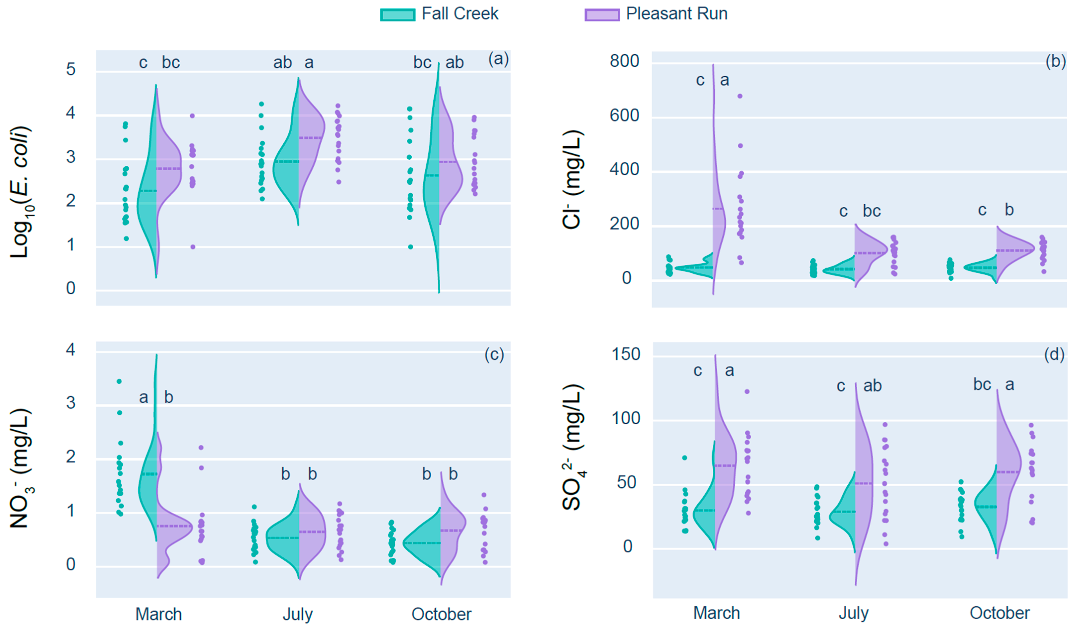
3.1. Long-Term and Seasonal Trends for log₁₀(E. coli), Cl⁻, NO₃⁻, and SO₄²⁻ from 2003 to 2021

No significant long-term trends (M-K test, p > 0.05) were observed for the concentration of log₁₀(E. coli), NO₃⁻, SO₄²⁻, and Cl⁻ in both Fall Creek and Pleasant Run from 2003 to 2021 (Figure 2). The variations in log₁₀(E. coli) exhibited fluctuating patterns with a range value of 2.27 to 4.03 for Fall Creek and 2.55 to 3.95 for Pleasant Run over time without a consistent upward or downward trend. Pleasant Run had higher log₁₀(E. coli) values than Fall Creek from 2011 to 2017, while the two streams possessed similar values at other times (Figure 2a). The Cl⁻ concentration fluctuated, and Pleasant Run had higher values (ranging from 67 to 274 mg/L) than Fall Creek (ranging from 36 to 78 mg/L) during the period (Figure 2b). Fall Creek displayed a higher NO₃⁻ concentration (ranging from 0.83 to 1.73 mg/L) compared to Pleasant Run (0.49 to 1.25 mg/L), although they shared similar dynamics (Figure 2c). The trends for SO₄²⁻ concentrations exhibited dynamic patterns, and the Pleasant Run had a higher range (26 to 87 mg/L) than Fall Creek (18 to 54 mg/L) (Figure 2d).

Significant seasonal differences were found for four water-quality parameters (Figure 3). Two-way ANOVA showed a significant difference in log₁₀(E. coli) values by sampling months (F = 10.38, p < 0.001) and by streams (F = 13.33, p < 0.001), while the impact from the interaction between sampling months and streams was not significant. A Tukey post-hoc test revealed significant pairwise differences between March and July, between July and October, and between Fall Creek and Pleasant Run for log₁₀(E. coli) values (Figure 3a). The Cl⁻ values had shown significant differences by sampling months (F = 19.43, p < 0.001) and by streams (F = 83.4, p < 0.001), and the interaction between sampling months and streams (F = 17.74, p < 0.001). Pairwise comparison revealed significantly higher Cl⁻ values in March than in July and October, as well as higher values in Pleasant Run than that in Fall Creek (Figure 3b). The NO₃⁻ values displayed significant differences by sampling months (F = 31.99, p < 0.001) and by streams (F = 6.70, p < 0.01), and by their interactions (F = 23.46, p < 0.001). NO₃⁻ concentration of Fall Creek in March showed higher values than any other group (Figure 3c). Significant differences were also found in SO₄²⁻ concentrations by streams (F = 56.05, p < 0.001), while the sampling month and the interaction between streams and sampling months were not significant (p > 0.05). Pleasant Run had higher SO₄²⁻ concentrations than Fall Creek (Figure 3d).

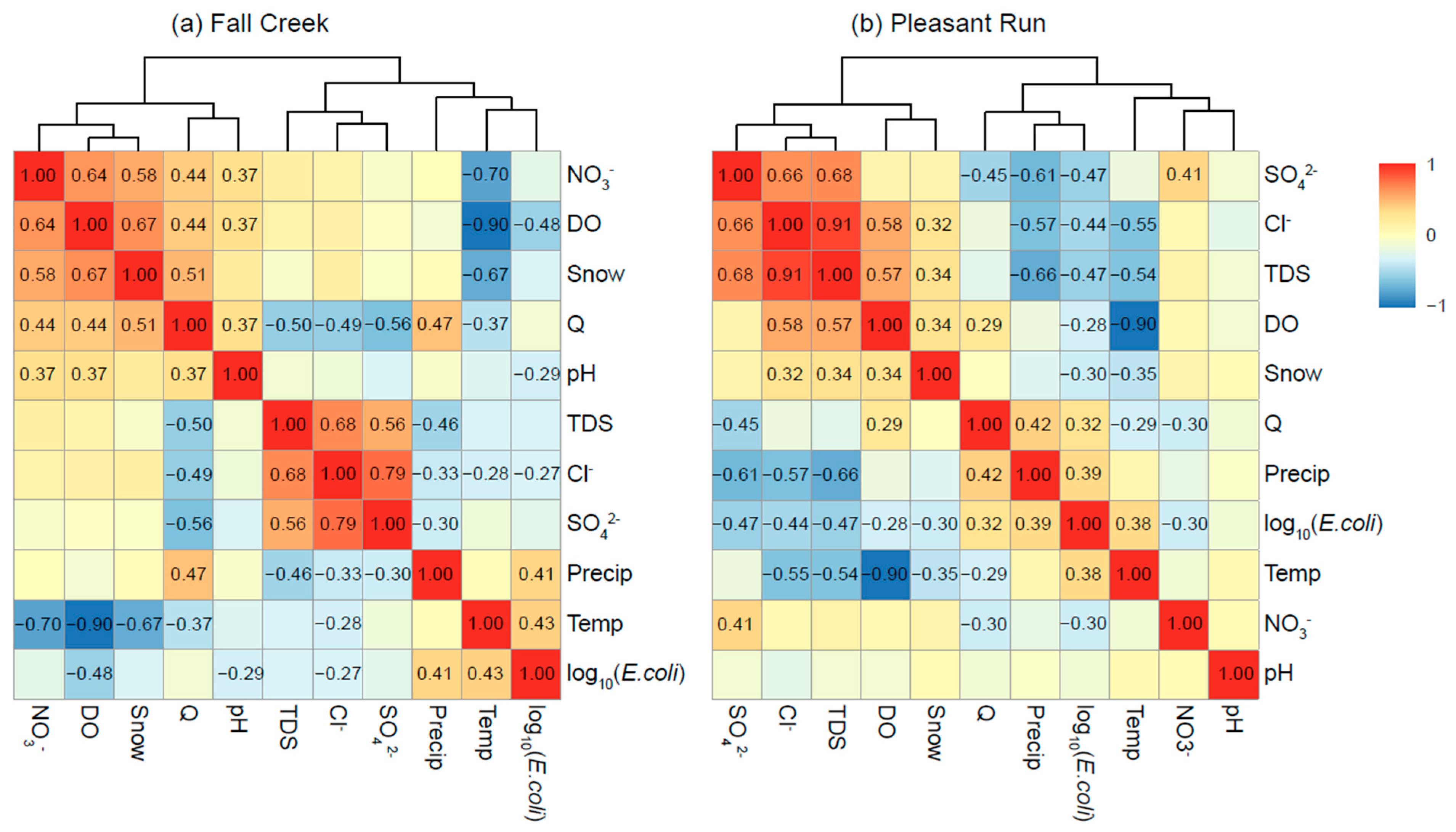
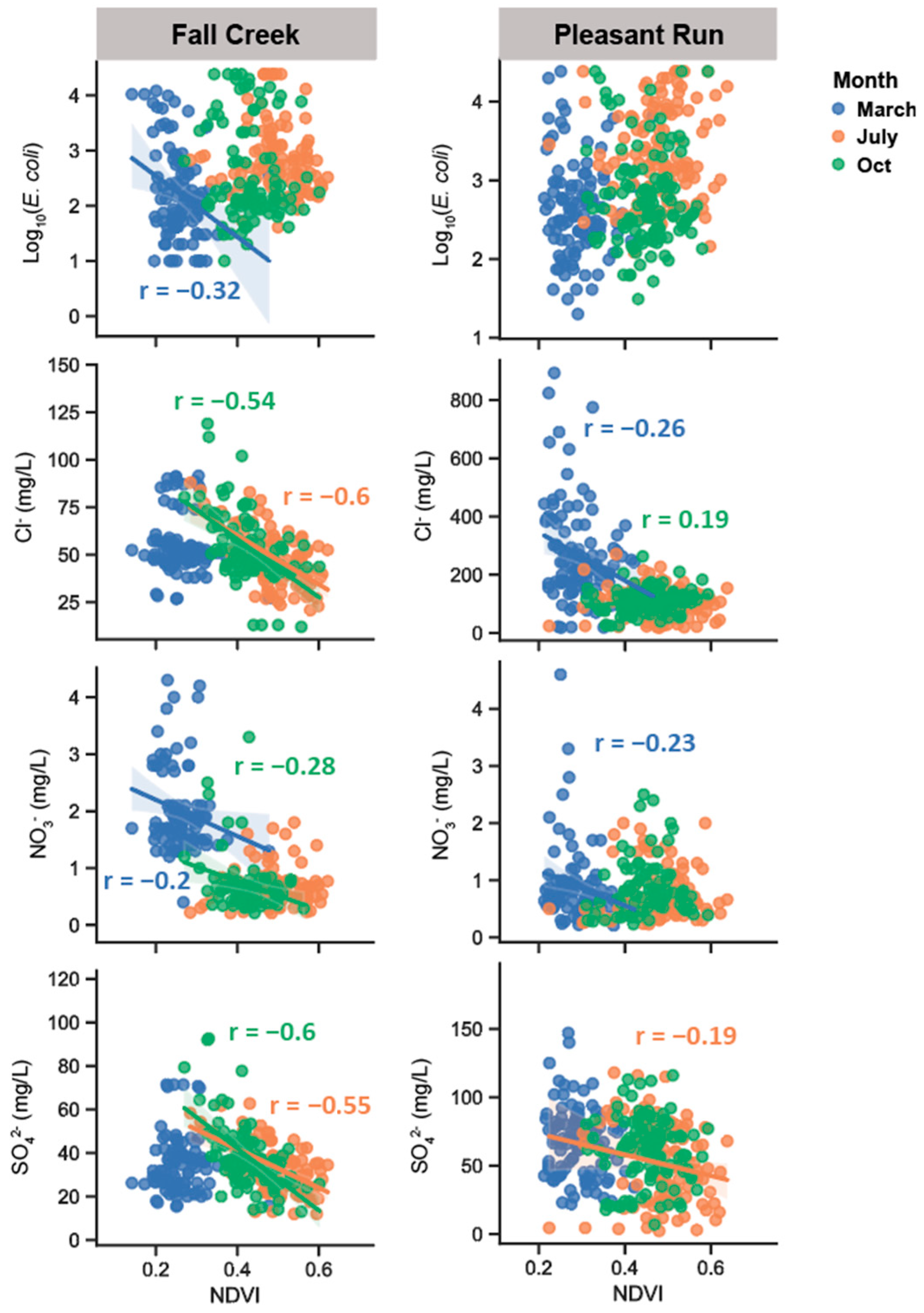
3.2. Relationships Between Water-Quality Variables and Potential Drivers over Time

Notable positive relationships were observed in Fall Creek between water temperature and log₁₀(E. coli) (r = 0.43, p < 0.05), log₁₀(E. coli) and 7-day antecedent precipitation (r = 0.41, p < 0.05), NO₃⁻ and 7-day antecedent snow (r = 0.64, p < 0.05), and TDS and SO₄²⁻ (r = 0.56, p < 0.05). Conversely, negative correlations were identified between DO and log₁₀(E. coli) (r = −0.48, p < 0.05), discharge and Cl⁻ (r = −0.49, p < 0.05), temperature and NO₃⁻ (r = −0.70, p < 0.05), and discharge and SO₄²⁻ (r = −0.56, p < 0.05) (Figure 4a). In Pleasant Run, significantly positive correlations occurred between TDS and SO₄²⁻ (r = 0.68, p < 0.05), TDS and Cl⁻ (r = 0.91, p < 0.05), 7-day antecedent snow and Cl⁻ (r = 0.32, p < 0.05), and water temperature and log₁₀(E. coli) (r = 0.38, p < 0.05). On the contrary, negative correlations were found between 7-day antecedent precipitation and Cl⁻ (r = −0.57, p < 0.05), 7-day antecedent precipitation and SO₄²⁻ (r = −0.61, p < 0.05), discharge and NO₃⁻ (r = −0.30, p < 0.05) (Figure 4b).

Cluster analysis revealed different group patterns of water-quality parameters in the two watersheds. In Fall Creek, Cl⁻, SO₄²⁻, and TDS exhibited stronger associations within the same cluster. Log₁₀(E. coli) demonstrated a higher level of similarity with 7-day antecedent precipitation and water temperature, while NO₃⁻ displayed more similarity with DO and 7-day antecedent snow (Figure 4a). Similarly, Cl⁻ displayed a close distance with SO₄²⁻ and TDS in Pleasant Run. In other groups, NO₃⁻ exhibited more similarity with temperature and pH. Seven-day antecedent precipitation and discharge were found to be more related to log₁₀(E. coli). Seven-day antecedent snow was grouped with DO (Figure 4b).

According to the RDA results, seven environmental variables: water temperature, pH, Q, TDS, DO, 7-day antecedent precipitation, and 7-day antecedent snow —can together explain up to 61% and 85% of the variances for water-quality parameters in Fall Creek and Pleasant Run, respectively (

Table 1. Total variance of log10(E. coli), Cl⁻, NO₃⁻, and SO₄²⁻ that can be explained by seven environmental variables. * and ** indicate a significance level of 0.05 and 0.01, respectively.

	Fall Creek
	log10(E.coli)			Cl−			NO3−			SO42−
Order	Variable	R2	Cumulated R2	Variable	R2	Cumulated R2	Variable	R2	Cumulated R2	Variable	R2	Cumulated R2
1	DO	0.182 **	0.182	TDS	0.478 **	0.478	Temp	0.537 **	0.537	TDS	0.276 **	0.276
2	Precip	0.133 **	0.315	Snow	0.055 *	0.53	Q	0.049 *	0.586	pH	0.031	0.307
3	pH	0.022	0.337	Precip	0.015	0.545	TDS	0.027 *	0.613	Precip	0.021	0.328
4	Q	0.007	0.344	DO	0.012	0.557	pH	0.023	0.636	DO	0.018	0.346
5	Temp	0.002	0.346	Temp	0.007	0.564	Precip	0.006	0.642	Snow	0.017	0.363
6				pH	0.006	0.57	Snow	0.002	0.646	Temp	0.003	0.366
7										Q	0.002	0.368
	Pleasant Run
	log10(E.coli)			Cl−			NO3−			SO42−
Order	Variable	R2	Cumulated R2	Variable	R2	Cumulated R2	Variable	R2	Cumulated R2	Variable	R2	Cumulated R2
1	TDS	0.235 **	0.235	TDS	0.651 **	0.651	Snow	0.254 **	0.254	TDS	0.400 **	0.400
2	DO	0.078 **	0.313	Snow	0.177 **	0.323	DO	0.007	0.261	DO	0.093 **	0.493
3	Q	0.068 *	0.381	pH	0.023 **	0.851	Q	0.006	0.267	Snow	0.032	0.525
4	Temp	0.027	0.408	Q	0.013	0.864	pH	0.003	0.27	Q	0.03	0.555
5	Precip	0.013	0.421	DO	0.006	0.87	TDS	0.003	0.273	Precip	0.017	0.572
6	pH	0.011	0.432				Temp	0.001	0.274	pH	0.004	0.576
7	Snow	0.002	0.434							Temp	0.002	0.578

). E. coli is strongly explained by higher TDS and DO concentrations, which could be related to more flow from the CSO events. Cl⁻ variations can be better explained by TDS and snow, which could indicate more salt runoff during snow-melting events. NO₃⁻ and SO₄²⁻ are likely affected by temperature, snow, and TDS, which might be due to fertilizer input from residential lawns near streams.

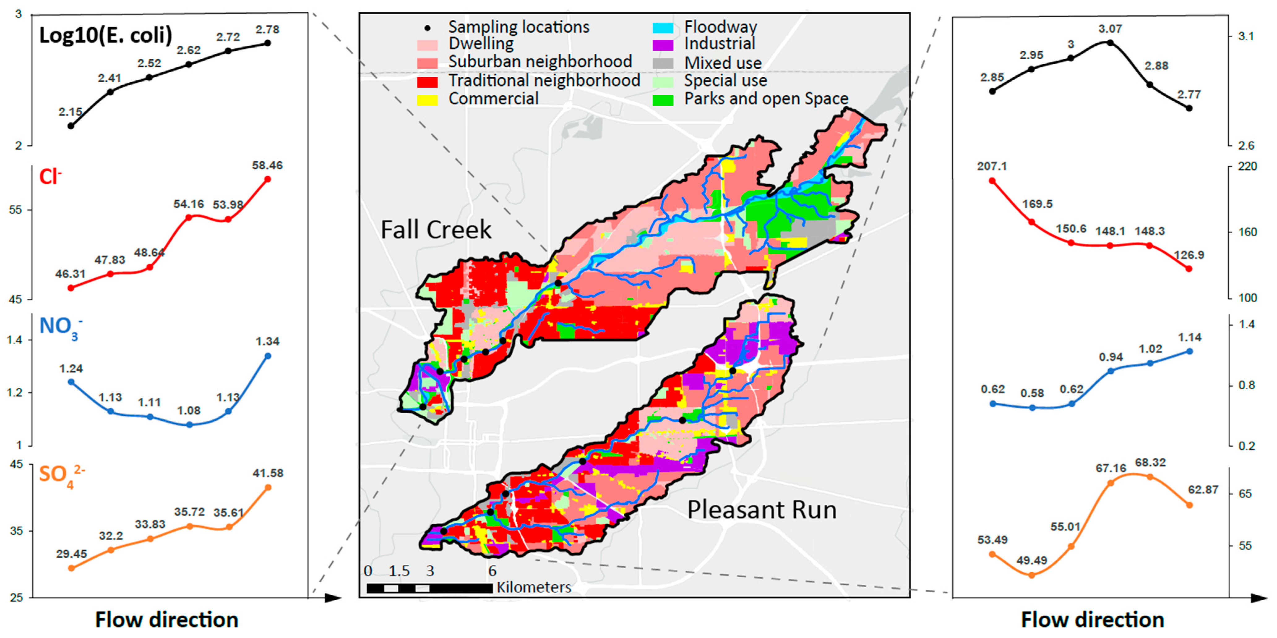
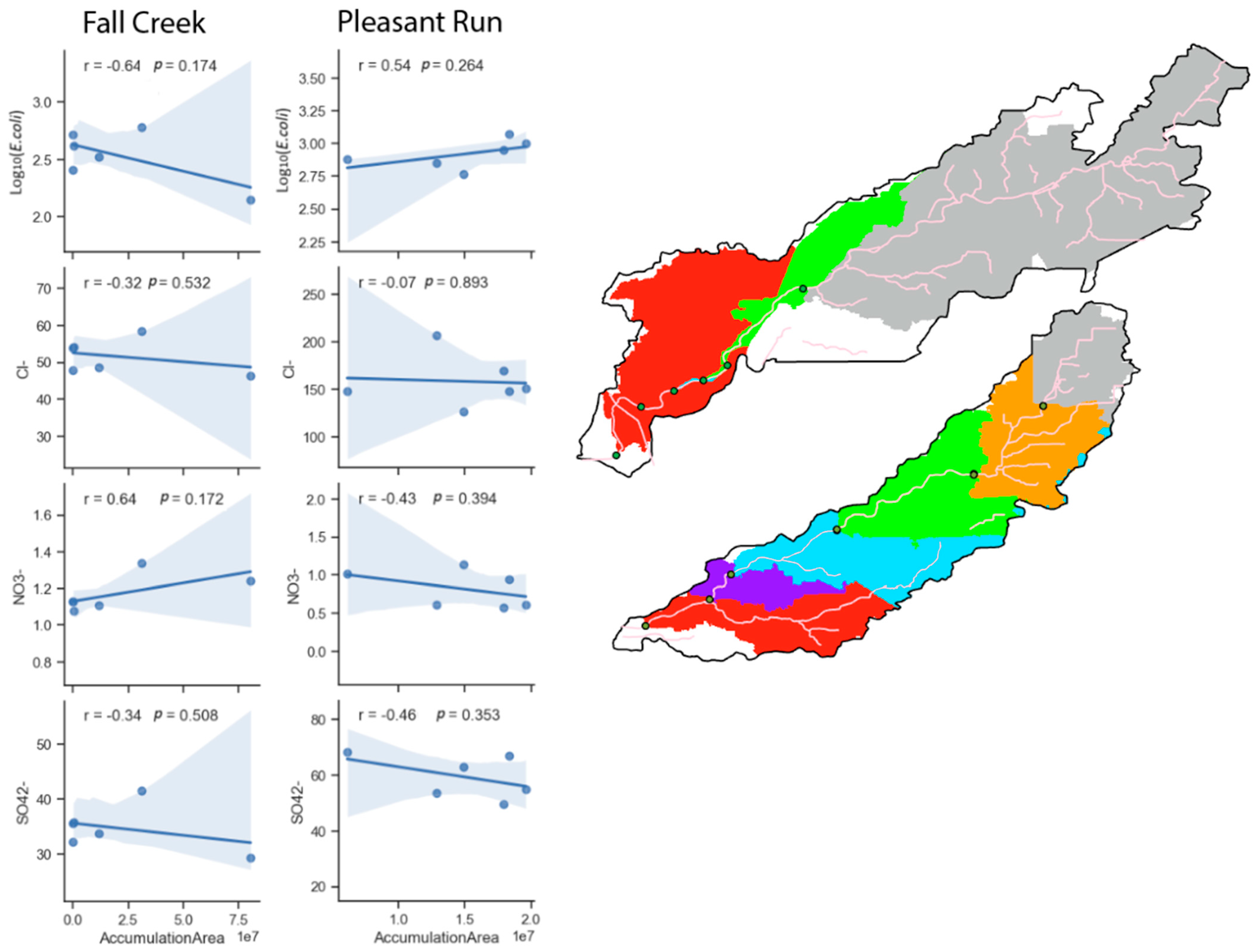
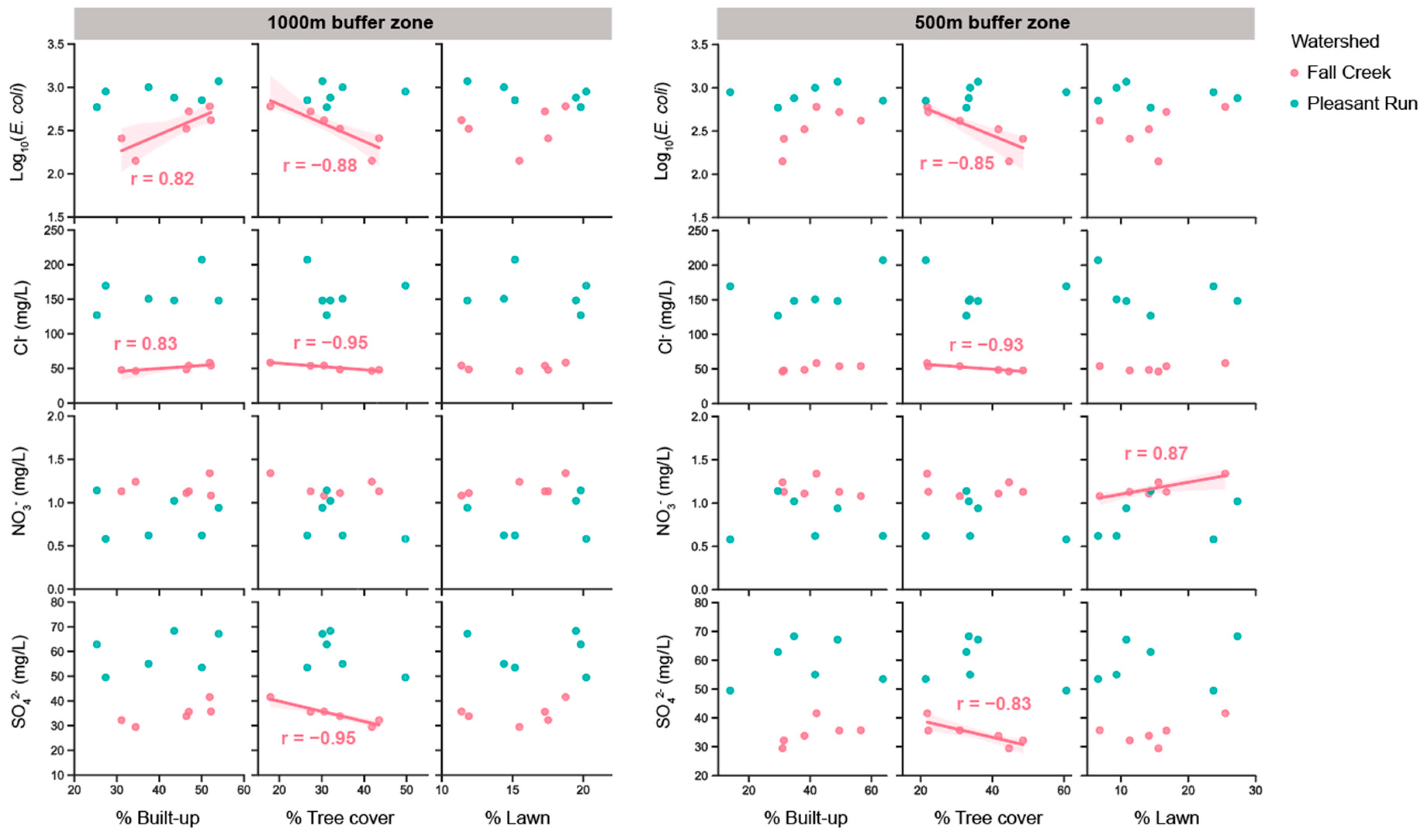
3.3. Spatial Patterns in Water-Quality Variables with Regards to Land-Use Factors

Along the flow direction, most parameters (e.g., log₁₀(E. coli), Cl⁻, NO₃⁻, and SO₄²⁻ in Fall Creek) had an increased trendline from upstream to downstream, while only a few trendlines (e.g., log₁₀(E. coli) and Cl⁻ in Pleasant Run) were decreasing towards downstream. Some of the locations downstream in Pleasant Run had lower values of water-quality parameters than upstream, which may be due to the dilution effects caused by the tributary flow (Figure 5). Specifically, Fall Creek had higher concentrations of chemicals and log₁₀(E. coli) downstream (Figure 5). In Pleasant Run, log₁₀(E. coli) and Cl⁻ concentration had higher values upstream, while NO₃⁻ and SO₄²⁻ showed higher concentrations at the downstream locations. Statistically, one-way ANOVA showed there were significant differences in log₁₀(E. coli), Cl⁻, NO₃⁻, and SO₄²⁻ concentration values between monitoring sites. In Fall Creek, sites 5 and 6 had significantly higher log₁₀(E. coli) values than site 1 (

Table 2. Mean values and standard deviations for log₁₀(E. coli) (E. coli unit: MPN/100 mL), concentrations of Cl⁻, NO₃⁻, and SO₄²⁻ at 12 sites. Same letters on superscripts represent differences between groups are not significant (p < 0.05).

Watershed	Site	Log10(E. coli)	Cl− (mg/L)	NO3− (mg/L)	SO42− (mg/L)
Fall Creek	Site 1	2.15 ± 0.54 b	46.31 ± 13 b	1.24 ± 0.95 a	29.45 ± 9 b
	Site 2	2.41 ± 0.85 ab	47.83 ± 13 b	1.13 ± 0.86 a	32.2 ± 10 b
	Site 3	2.52 ± 0.81 ab	48.64 ± 13 b	1.11 ± 0.8 a	33.83 ± 10 b
	Site 4	2.62 ± 0.87 ab	54.16 ± 14 ab	1.08 ± 0.85 a	35.72 ± 10 ab
	Site 5	2.72 ± 0.89 a	53.98 ± 15 ab	1.13 ± 0.8 a	35.61 ± 11 ab
	Site 6	2.78 ± 0.78 a	58.46 ± 21 a	1.34 ± 0.86 a	41.58 ± 18 a
Pleasant Run	Site a	2.85 ± 0.6 a	207.11 ± 170 a	0.62 ± 0.68 b	53.49 ± 25 bc
	Site b	2.95 ± 0.68 a	169.51 ± 135 ab	0.58 ± 0.27 b	49.49 ± 21 c
	Site c	3 ± 0.76 a	150.59 ± 118 ab	0.62 ± 0.4 b	55.01 ± 23 abc
	Site d	3.07 ± 0.64 a	148.09 ± 112 ab	0.94 ± 0.5 a	67.16 ± 30 ab
	Site e	2.88 ± 0.7 a	148.28 ± 105 ab	1.02 ± 0.55 a	68.32 ± 29 a
	Site f	2.77 ± 0.69 a	126.93 ± 78 b	1.14 ± 0.51 a	62.87 ± 25 abc

). Site 6 had significantly higher Cl− and SO₄²⁻ concentrations than sites 1–3. In Pleasant Run, site a had higher Cl⁻ values than site f, sites d–f had higher NO₃⁻ than sites a–c, and site e had higher SO₄²⁻ values than site b (Table 2).

There was no significant relationship between water-quality parameters and individual sub-watershed runoff area (Figure 6), which may suggest urban runoff is too complex to be explained only by surface runoff since urban streams are quite different from natural rivers due to the addition of drainage systems in cities. In terms of land cover impacts on water-quality parameters (Figure 7), more urban built-up areas were correlated with higher concentrations of E. coli and Cl⁻, higher tree cover was associated with lower concentrations of E. coli, Cl⁻, and SO₄²⁻, potentially resulting from reduced runoff. Increased use of fertilizers may explain the positive correlation between NO₃⁻ and lawn cover. Cl⁻ is hypothesized to originate from the road salt applied on the streets during the winter, but no significant relationships were found between Cl⁻ concentration and street length/parking lot area in 1000 or 500 m buffers (Figure S3). Comparing the associations of different land-use types with water-quality parameters, higher chloride values were associated with commercial areas, elevated nitrate concentration was associated with higher residential density, and increased sulfate levels were observed at sampling locations surrounded by a higher amount of industrial land use. However, results at both buffer and sub-watershed scales (Figure S4) did not reveal statistically significant results between land-use parameters (residential, commercial, industrial, parks) and water-quality variables.

In Fall Creek, there were negative relationships between log₁₀(E. coli) and NDVI, and Cl⁻ and NDVI in July and October. In Pleasant Run, negative relationships occurred between Cl⁻ and NDVI, and NO₃⁻ and NDVI in March (Figure 8). The results of the negative relationships between NDVI and water-quality variables are consistent with the hypothesis of tree cover mitigating the water pollution, regardless of which season.

4. Discussion

4.1. Mechanisms of Changing Climate on Urban Stream Water Quality

While investigating urban water environment and stormwater contamination sources under the impact of changing climate, the assessment of E. coli, Cl⁻, NO₃⁻, and SO₄²⁻ concentrations has been prevalent to identify the water-quality condition. Previous studies have reported distinct seasonal trends in these parameters [2,20,21,22,23]. Our study similarly revealed significant temporal variations (p < 0.01) in water-quality parameters across seasons (Figure 3), primarily attributed to changing climate and contaminant sources [24]. Notably, climatic factors such as precipitation and temperature, peaking in summer, correlated with the highest E. coli concentration in July in Pleasant Run [25]. Moreover, E. coli concentrations exhibited strong associations with DO and specific conductivity, paired with climatic factors, making them reliable predictors of E. coli presence over time [26]. The Cl⁻ concentration exhibited a higher value during winter in both streams, with the value being above 250 mg/L, posing a threat to freshwater ecosystems [27]. Cl⁻ concentration also positively correlated with the amount of snow (Figure 4), suggesting that more salt would be used on the road, which contributes to higher levels of Cl⁻ in streams in March. The origins of NO₃⁻ and SO₄²⁻ were potentially traced to organic processes in soil and drainage from lawn care and landfills [28]. Although SO₄²⁻ displayed no obvious seasonal pattern, they were partially related to the amount of precipitation and snow. A comparative result of two watersheds indicated a lower Cl⁻ concentration in Fall Creek, suggesting a potential dilution effect attributable to its higher discharge volume.

Regarding analyzing the influences of climatic and environmental factors on water quality, multiple analyses, including cluster analysis and other multivariate analysis techniques (RDA), have been used to identify determinants of water-quality variability [29]. They found that land-use patterns can explain up to 68% of water-quality variations. Our RDA analysis displayed the water-quality relationships with climatic and hydrologic parameters. Seven environmental variables—water temperature, pH, stream discharge, total dissolved solids (TDS), dissolved oxygen (DO), snow amount, and precipitation—collectively account for up to 61% and 85% of the variances for Fall Creek and Pleasant Run over time, respectively. Similarly, more studies have discussed the relationship between water quality, climate, land use, and hydrological characteristics. For example, land-use, topography, and social-economic factors can explain the overall water quality from RDA results where urban land use was found to be the most important factor explaining water quality [30]. It shows that precipitation, temperature, and streamflow can explain the dynamics of water-quality parameters in the Cuyahoga River basin of Lake Erie [31]. Additionally, [32] also conducted an RDA analysis, and they found land use, landscape metrics, and hydrological parameters, plus NDVI, can collectively account for water-quality variations.

4.2. Mechanisms of Land Use on Urban Stream Water Quality

Land use affects water quality by changing surface runoff patterns, modifying sanitary sewer overflow, and introducing additional pollutants resulting from diverse human activities. First, while changing climate impacts surface runoff through increased precipitation, urban land use contributes to surface runoff by introducing impervious surfaces such as rooftops, driveways, parking lots, and paved streets. Second, urban land use has strong implications for sanitary/combined sewer overflow as the system becomes overwhelmed through urban runoff. Third, each land-use component contributes different contamination sources that impact water quality. Residential lawn cover appears to have more nitrate due to fertilizing, commercial streets and parking lots have more chloride due to de-icing road salt in the winter, and industrial activities may result in more sulfate [6,7,33,34]. Our results basically reported a stronger correlation between NO₃⁻ and residential zones, indicating a potential contribution from lawn fertilizers. These pollutants result in contaminated water bodies in urban environments.

Land-cover proportions (urban built-up, tree cover, lawn cover) were significantly related to water-quality parameters in the current study. Other studies also found similar results. In Lake Muhazi, Rwanda, despite urban built-up areas constituting the smallest proportion among land-cover types, it exhibited a strong association with fecal coliform input, particularly during the rainy season. This correlation was attributed to human activities, such as livestock and point source contamination [35]. Another spatial analysis of water-quality parameters was conducted in South Korea. It was found that urban land cover is positively correlated with the increase in urban water pollution [33].

NDVI was considered a useful indicator for water-quality conditions [5]. Higher NDVI represents more greenness and more dense vegetation, which might affect nutrient uptake and chemical transport in different seasons. In our study, negative relationships were found between NDVI and water-quality parameters during March, July, and October, suggesting that more tree cover or more vegetation can cause less runoff into the river, which can potentially mitigate the water contamination.

The modifiable areal unit problem (MAUP) is an issue that could affect the results of spatial analysis in water quality when drawing different geographic boundaries around each sampling site [36] as different boundaries have been shown to produce variable results. Previous studies have attempted to mitigate the effects of MAUP to identify the appropriate spatial extent for assessing land-use impacts. Sub-watersheds and buffers of varying sizes around sampling locations have been used to examine land-use and water-quality relationships (e.g., [33,37,38]). For example, in the Han River basin of South Korea, water-quality parameters, such as biochemical/chemical oxygen demand, suspended sediment, total phosphorus, and total nitrogen, were better explained by land cover summarized within 100 m buffers, while DO was more highly correlated with land cover within the whole watershed [33]. In major river systems of the Zhejiang province, China, when looking at the relationship between percent land-use types and water quality, sub-watershed analysis was superior. However, a 500 m buffer was more appropriate when comparing the variability of nutrients with land-cover types [38]. While these studies found that using 100 m and 500 m buffers was more effective for their study areas, our study showed mixed results. A 1000 m buffer was more effective in capturing the relationship between water quality and urban built-up areas/tree cover, while a 500 m buffer could explain relationships between nitrate levels and urban lawn cover. Further, the sub-watershed analysis proved inadequate when trying to capture the spatial extent of pollutant contribution to our sampling location, as the area of each sub-watershed did not proportionally correlate with water-quality levels on our sites. This implies that circular buffers around sampling locations were better for the sub-watershed scale when using land-use variables to explain water-quality variations in our case. This is likely because the discharge from underground drainage systems (e.g., storm drains, combined sewer systems), which is related to urban infrastructure settings, is not considered for sub-watershed analyses due to the challenges to accurately map the underground drainage systems in urban environments.

4.3. Limitations and Management Implications

This study focuses on Indianapolis, a midwestern U.S. city with a combined sewer system and seasonal rainfall variability. The city has invested in long-term water-quality monitoring, making it a data-rich environment to investigate high spatial and temporal variability in water quality. For temporal water-quality analysis, our linear model provided useful relationships for identifying changing climate, land-use, and water-quality relationships. The method applies to urban water systems worldwide that face similar challenges, such as nutrient loading, land-use pressures, and stormwater impacts. However, there are uncertainties and limitations with the methods. Linear regression has been used to detect relationships. In here, more environmental factors, especially climatic data, can be collected, such as snow amount, snow/rainfall frequency, and runoff volume, to obtain a higher R² value of the linear model so we can have better prediction power. Also, some of the relationships between water-quality parameters and environmental predictors may not be linear, requiring non-linear models.

When investigating the influence of land use (e.g., residential, commercial, and industrial areas) on water quality, the variability of water-quality parameters is related to these land-use categories. For example, a higher density of residential areas leads to an increased level of E. coli. But no linear relationships were found within specific buffer zones in our study area. The lack of significant linear relationships indicated a less defined spatial trend between land use and water quality within a complex urban system. In addition, the expected positive relationship between Cl⁻ and urban features such as street densities, parking lots, or impervious area/indexes was not found in our case. Since parking lot/street salt is a significant source of Cl⁻ contamination during the winter, the suggestion for future study is to classify urban features specifically, such as investigating the types and densities of street networks. Also, exploring alternative methods for delineating the distribution of Cl⁻ runoff, beyond buffer scale and sub-watershed analysis, can help better understand the spread of Cl⁻ in urban areas.

When it comes to land-cover impacts, first, our study has explored different land-cover elements (e.g., urban built-up, tree cover, lawn cover) and highlighted the significant contribution of urban land-to-water-quality degradation. However, due to the rapid pace of urban development, especially concerning the impacts of combined sewer overflows and human activities, urban storm and sewer infrastructure information such as hydraulic data (pipes and drains) need to be incorporated in modeling to account for sources more explicitly, as it would allow for a more comprehensive analysis of the spatial patterns in urban water quality. Second, our analysis has revealed the relationship between water quality and NDVI. There is potential to explore more NDVI datasets, offering a high-resolution view both temporally and spatially. It can provide broad insights into this specific environmental indicator of water quality. Third, expanding our analysis to integrate more geographical data, such as population density, can enrich the understanding of the interaction between human activities and water quality. Mitigating the urban land impacts on streams requires regulating urban community practices and investing in environmentally friendly infrastructure.

The severity of urban stormwater pollution is influenced by factors such as population density, urbanization, runoff area, age of stormwater infrastructure, and the amount of road salt/fertilizer application. Our study found that sub-watershed basins could not relate to the entire variability of chemical dynamics, emphasizing the importance of the underlying urban drainage system, which plays a critical role in transporting pollutants into streams. To effectively identify source distribution and manage pollution runoff, it is essential to conduct additional buffer/sub-watershed analysis at varying scales, as well as examine the underlying drainage network, like stormwater channels, pipes, and sewer lines/basins. This approach can help pinpoint specific sources of pollution. Strategies such as reducing the use of lawn fertilizers and road salt during urban planning and construction processes may also be beneficial. Ultimately, addressing the changing climate, land-use, and water-quality problems requires the development of climate-resilient infrastructure and the implementation of low-impact development practices, particularly in urban areas.

5. Conclusions

Urban stream water quality (including E. coli, Cl⁻, NO₃⁻, SO₄²⁻) was investigated concerning its spatiotemporal pattern and the influences of climate and land use in Indianapolis. The results revealed that July had higher E. coli values than other months, possibly due to a higher amount of rainfall and higher temperatures in summer. March had higher levels of Cl⁻ in Pleasant Run due to runoff from urban areas during the winter season or snow-melting events. NO₃⁻/SO₄²⁻ concentrations stand out significantly in March, indicating an increase in fertilizer application near streams or wastewater input into rivers by humans living nearby. Urban built-up and lawn cover are positively related to the variations of water-quality variables, while tree cover and NDVI are negatively correlated with water-quality dynamics. With variations in the water-quality parameters and the complexity of influences of changing climate and land use, proper management strategies need to be implemented with regard to not only focusing on changing climate mitigation but also on urban land types and human practices if we want our waterways to remain safe.

Circular buffers and sub-watershed scale analysis delineate the possible spatial runoff extent of pollutants to each sampling site within urban watersheds. A 1000 m buffer was more effective in capturing the relationship between water-quality parameters (i.e., E. coli and Cl⁻) and urban built-up areas/tree cover, while a 500 m buffer scale could explain relationships between nitrate levels and urban lawn cover. Our study contributes to the knowledge of the spatial distribution of contaminant runoff to urban streams. It helps to understand urban stream water-quality responses to future changes of urban land cover/use, which will ensure the resilience of urban stream ecosystems and safeguard water quality for human and ecological health.

References

1. Alamdari, N.; Sample, D.J.; Ross, A.C.; Easton, Z.M. Evaluating the Impact of Climate Change on Water Quality and Quantity in an Urban Watershed Using an Ensemble Approach. Estuaries Coasts 2020, 43, 56–72. [Google Scholar] [CrossRef]
2. Adeola Fashae, O.; Abiola Ayorinde, H.; Oludapo Olusola, A.; Oluseyi Obateru, R. Landuse and surface water quality in an emerging urban city. Appl. Water Sci. 2019, 9, 1–12. [Google Scholar] [CrossRef]
3. Ingram, W. Increases all round. Nat. Clim. Change 2016, 6, 443–444. [Google Scholar] [CrossRef]
4. Whitehead, P.G.; Wilby, R.L.; Battarbee, R.W.; Kernan, M.; Wade, A.J. A review of the potential impacts of climate change on surface water quality. Hydrol. Sci. J. 2009, 54, 101–123. [Google Scholar] [CrossRef]
5. Griffith, J.A.; Martinko, E.A.; Whistler, J.K.; Price, K.P. Interrelationships among landscapes, NDVI, and stream water quality in the U.S. Central Plains. Ecol. Appl. 2002, 12, 1702–1718. [Google Scholar] [CrossRef]
6. Yang, Y.Y.; Toor, G.S. Sources and mechanisms of nitrate and orthophosphate transport in urban stormwater runoff from residential catchments. Water Res. 2017, 112, 176–184. [Google Scholar] [CrossRef]
7. Davis, B.; Birch, G. Comparison of heavy metal loads in stormwater runoff from major and minor urban roads using pollutant yield rating curves. Environ. Pollut. 2010, 158, 2541–2545. [Google Scholar] [CrossRef]
8. Brezonik, P.L.; Stadelmann, T.H. Analysis and predictive models of stormwater runoff volumes, loads, and pollutant concentrations from watersheds in the Twin Cities metropolitan area, Minnesota, USA. Water Res. 2002, 36, 1743–1757. [Google Scholar] [CrossRef]
9. Gilbert, J.K.; Clausen, J.C. Stormwater runoff quality and quantity from asphalt, paver, and crushed stone driveways in Connecticut. Water Res. 2006, 40, 826–832. [Google Scholar] [CrossRef]
10. Mora, A.; Mahlknecht, J.; Rosales-Lagarde, L.; Hernández-Antonio, A. Assessment of major ions and trace elements in groundwater supplied to the Monterrey metropolitan area, Nuevo León, Mexico. Environ. Monit. Assess. 2017, 189, 1–15. [Google Scholar] [CrossRef]
11. Pfaff, J.D. Determination of Inorganic Anions by Ion Chromatography. EPA Method 300. 1993. Available online: https://www.epa.gov/sites/default/files/2015-08/documents/method_300-0_rev_2-1_1993.pdf (accessed on 1 June 2022).
12. Zanaga, D.; Van De Kerchove, R.; Daems, D.; De Keersmaecker, W.; Brockmann, C.; Kirches, G.; Wevers, J.; Cartus, O.; Santoro, M.; Fritz, S.; et al. ESA WorldCover 10 m 2021 v200. 2022. Available online: https://pure.iiasa.ac.at/id/eprint/18478/ (accessed on 1 June 2022). [CrossRef]
13. Corbin, T. Learning ArcGIS Pro; Packt Publishing Ltd.: Birmingham, UK, 2015. [Google Scholar]
14. Qiao, N.; Wang, L. Satellite observed vegetation dynamics and drivers in the Namib sand sea over the recent 20 years. Ecohydrology 2022, 15, e2420. [Google Scholar] [CrossRef]
15. Zhang, Y.; Gentine, P.; Luo, X.; Lian, X.; Liu, Y.; Zhou, S.; Michalak, A.M.; Sun, W.; Fisher, J.B.; Piao, S.; et al. Increasing sensitivity of dryland vegetation greenness to precipitation due to rising atmospheric CO2. Nat. Commun. 2022, 13, 4875. [Google Scholar] [CrossRef]
16. Jiao, W.; Wang, L.; Smith, W.K.; Chang, Q.; Wang, H.; D’Odorico, P. Observed increasing water constraint on vegetation growth over the last three decades. Nat. Commun. 2021, 12, 3777. [Google Scholar] [CrossRef] [PubMed]
17. Zhang, X.; Zhao, W.; Wang, L.; Liu, Y.; Liu, Y.; Feng, Q. Relationship between soil water content and soil particle size on typical slopes of the Loess Plateau during a drought year. Sci. Total Environ. 2019, 648, 943–954. [Google Scholar] [CrossRef] [PubMed]
18. Kluyver, T.; Ragan-Kelley, B.; Pérez, F.; Granger, B.; Bussonnier, M.; Frederic, J.; Kelley, K.; Hamrick, J.; Grout, J.; Corlay, S.; et al. Jupyter Notebooks-a publishing format for reproducible computational workflows. In Positioning and Power in Academic Publishing: Players, Agents and Agendas; IOS Press: Amsterdam, The Netherlands, 2016; Volume 2016, pp. 87–90. [Google Scholar] [CrossRef]
19. Waskom, M.L. Seaborn: Statistical data visualization. J. Open Source Softw. 2021, 6, 3021. [Google Scholar] [CrossRef]
20. Bernal, S.; Butturini, A.; Sabater, F. Inferring nitrate sources through end member mixing analysis in an intermittent Mediterranean stream. Biogeochemistry 2006, 81, 269–289. [Google Scholar] [CrossRef]
21. Chen, H.J.; Chang, H. Response of discharge, TSS, and E. coli to rainfall events in urban, suburban, and rural watersheds. Environ. Sci. Process Impacts 2014, 16, 2313–2324. [Google Scholar] [CrossRef]
22. Gardner, K.M.; Royer, T.V. Effect of Road Salt Application on Seasonal Chloride Concentrations and Toxicity in South-Central Indiana Streams. J. Environ. Qual. 2010, 39, 1036–1042. [Google Scholar] [CrossRef]
23. Ledford, S.H.; Lautz, L.K. Floodplain connection buffers seasonal changes in urban stream water quality. Hydrol. Process 2015, 29, 1002–1016. [Google Scholar] [CrossRef]
24. Vermeulen, L.C.; Hofstra, N. Influence of climate variables on the concentration of Escherichia coli in the Rhine, Meuse, and Drentse Aa during 1985–2010. Reg. Environ. Change 2014, 14, 307–319. [Google Scholar] [CrossRef]
25. Li, R.; Filippelli, G.; Wang, L. Annual Precipitation and Discharge Drive Increases in Escherichia Coli Concentrations in an Urban Stream. Sci. Total Environ. 2023, 886, 163892. [Google Scholar] [CrossRef] [PubMed]
26. Graves, G.M.; Vogel, J.R. Spatiotemporal Variability Comparisons of Water Quality and Escherichia coli in an Oklahoma Stream. J. Contemp. Water Res. Educ. 2023, 177, 94–102. [Google Scholar] [CrossRef]
27. Kaushal, S.S.; Groffman, P.M.; Likens, G.E.; Belt, K.T.; Stack, W.P.; Kelly, V.R.; Band, L.E.; Fisher, G.T. Increased salinization of fresh water in the northeastern United States. Proc. Natl. Acad. Sci. USA 2005, 102, 13517–13520. [Google Scholar] [CrossRef]
28. Khatri, N.; Tyagi, S. Influences of natural and anthropogenic factors on surface and groundwater quality in rural and urban areas. Front. Life Sci. 2015, 8, 23–39. [Google Scholar] [CrossRef]
29. Shi, P.; Zhang, Y.; Li, Z.; Li, P.; Xu, G. Influence of land use and land cover patterns on seasonal water quality at multi-spatial scales. Catena 2017, 151, 182–190. [Google Scholar] [CrossRef]
30. Chen, J.; Lu, J. Effects of land use, topography and socio-economic factors on river water quality in a mountainous watershed with intensive agricultural production in East China. PLoS ONE 2014, 9, e102714. [Google Scholar] [CrossRef] [PubMed]
31. Wang, R.; Ma, Y.; Zhao, G.; Zhou, Y.; Shehab, I.; Burton, A. Investigating water quality sensitivity to climate variability and its influencing factors in four Lake Erie watersheds. J. Environ. Manag. 2023, 325, 116449. [Google Scholar] [CrossRef]
32. Xu, G.; Li, P.; Lu, K.; Tantai, Z.; Zhang, J.; Ren, Z.; Wang, X.; Yu, K.; Shi, P.; Cheng, Y. Seasonal changes in water quality and its main influencing factors in the Dan River basin. Catena 2019, 173, 131–140. [Google Scholar] [CrossRef]
33. Chang, H. Spatial analysis of water quality trends in the Han River basin, South Korea. Water Res. 2008, 42, 3285–3304. [Google Scholar] [CrossRef]
34. Torres-Martínez, J.A.; Mora, A.; Knappett, P.S.K.; Ornelas-Soto, N.; Mahlknecht, J. Tracking nitrate and sulfate sources in groundwater of an urbanized valley using a multi-tracer approach combined with a Bayesian isotope mixing model. Water Res. 2020, 182, 115962. [Google Scholar] [CrossRef]
35. Umwali, E.D.; Kurban, A.; Isabwe, A.; Mind’je, R.; Azadi, H.; Guo, Z.; Udahogora, M.; Nyirarwasa, A.; Umuhoza, J.; Nzabarinda, V.; et al. Spatio-seasonal variation of water quality influenced by land use and land cover in Lake Muhazi. Sci. Rep. 2021, 11, 17376. [Google Scholar] [CrossRef] [PubMed]
36. Dark, S.J.; Bram, D. The modifiable areal unit problem (MAUP) in physical geography. Prog. Phys. Geogr. 2007, 31, 471–479. [Google Scholar] [CrossRef]
37. Tang, W.; Lu, Z. Application of self-organizing map (SOM)-based approach to explore the relationship between land use and water quality in Deqing County, Taihu Lake Basin. Land Use Policy 2022, 119, 106205. [Google Scholar] [CrossRef]
38. Gu, Q.; Hu, H.; Ma, L.; Sheng, L.; Yang, S.; Zhang, X.; Zhang, M.; Zheng, K.; Chen, L. Characterizing the spatial variations of the relationship between land use and surface water quality using self-organizing map approach. Ecol. Indic. 2019, 102, 633–643. [Google Scholar] [CrossRef]
Figure 1. Map of Fall Creek Watershed and Pleasant Run Watershed in Indianapolis showing the location of water-quality monitoring stations and land-cover types in 2021. Numbers 1–6 are sampling sites along Fall Creek, letters a–f are sampling sites along Pleasant Run.
Water 17 01225 g001
Figure 2. Long-term trends of log10(E. coli) (E. coli concentration unit: MPN/100 mL) (a), concentrations of Cl (b), NO3 (c), SO42− (d) from 2003 to 2021. Mann–Kendall (M–K) statistical test is to detect the presence and direction of a monotonic trend (upward or downward) in a time series variable.
Water 17 01225 g002
Figure 3. Difference of log10(E. coli) (a), concentrations of Cl (b), NO3 (c), and SO42− (d) in three seasons and two watersheds. Dashed lines are the mean values of each group. Same letters on the bar reflect that differences between groups are not significant (p < 0.05).
Water 17 01225 g003
Figure 4. Spearman correlation matrix with hierarchical clustering of water-quality parameters and environmental factors for (a) Fall Creek and (b) Pleasant Run streams. In the heatmap, warm colors represent positive correlation, while cool colors represent negative correlation. The number on each shade represents the significant (p < 0.05) correlation coefficients, which range from −1 to 1. Dendrograms group together the variables that have similarities. E. coli: MPN/100 mL; Cl: mg/L; NO3: mg/L; SO42−: mg/L; TDS: total dissolved solid (g/L); Q: discharge (m3/s); Temp: water temperature (°C); DO: dissolved oxygen (mg/L); Precip: 7-day antecedent precipitation (mm); Snow: 7−day antecedent snow (mm).
Water 17 01225 g004
Figure 5. Spatial pattern of water-quality parameters from upstream to downstream and land-use types in two watersheds. (data.indy.gov/datasets/IndyGIS::dmd-land-use-plan-base/explore (accessed on 1 August 2022)) E. coli: MPN/100 mL; Cl: mg/L; NO3: mg/L; SO42−: mg/L.
Water 17 01225 g005
Figure 6. Sub-watershed for individual sampling location and their relationships with stream chemical concentrations. The lines represent regression lines that summarize the relationship between scatter points. Light blue shades represent 95% confidence interval on the regression line. Dots on diagram (left to right) correspond to the dots (right to left) on the map.
Water 17 01225 g006
Figure 7. Relationships between water-quality parameters and land-use types at 1000 m and 500 m buffer scale near each of 12 total sites. Only significant (p < 0.05) linear regression line was shown on each panel. E. coli unit: MPN/100 mL.
Water 17 01225 g007
Figure 8. Relationships between water-quality parameters and NDVI values at a 1000 m buffer zone around each of the 12 total sites. Only significant (p < 0.05) linear regression line was shown on each panel. E. coli unit: MPN/100 mL. Normalized Difference Vegetation Index (NDVI) is an effective index that uses satellite data to assess vegetation cover and health. r value is the correlation coefficient, it quantifies the strength and direction of a linear relationship between two variables, ranging from −1 to +1. Values closer to 1 (positive or negative) indicate stronger correlations (positive or negative, respectively).
Water 17 01225 g008