
Prediction of Shallow Landslide Runout Distance Based on Genetic Algorithm and Dynamic Slicing Method


Abstract
:1. Introduction
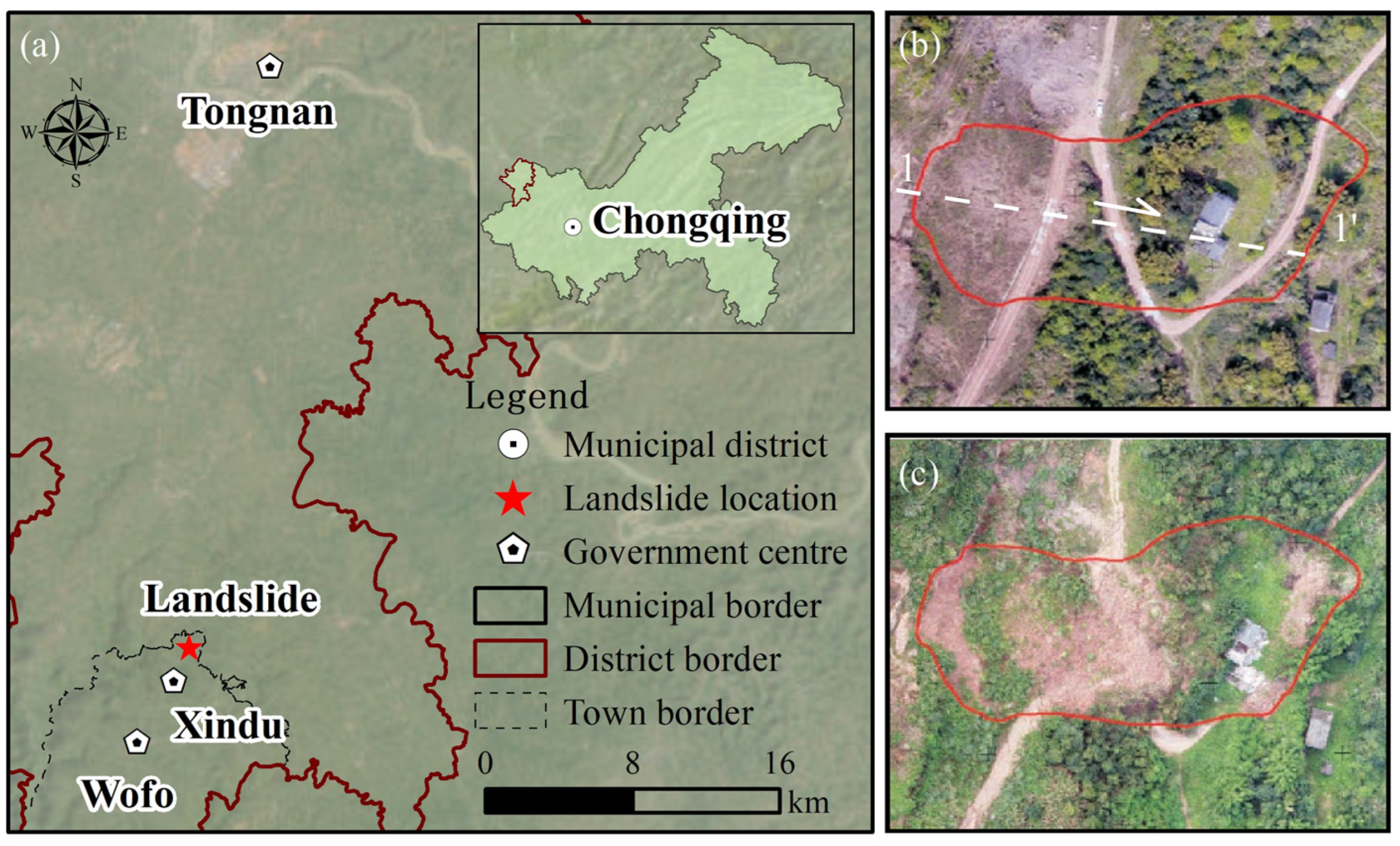
2. Study Area
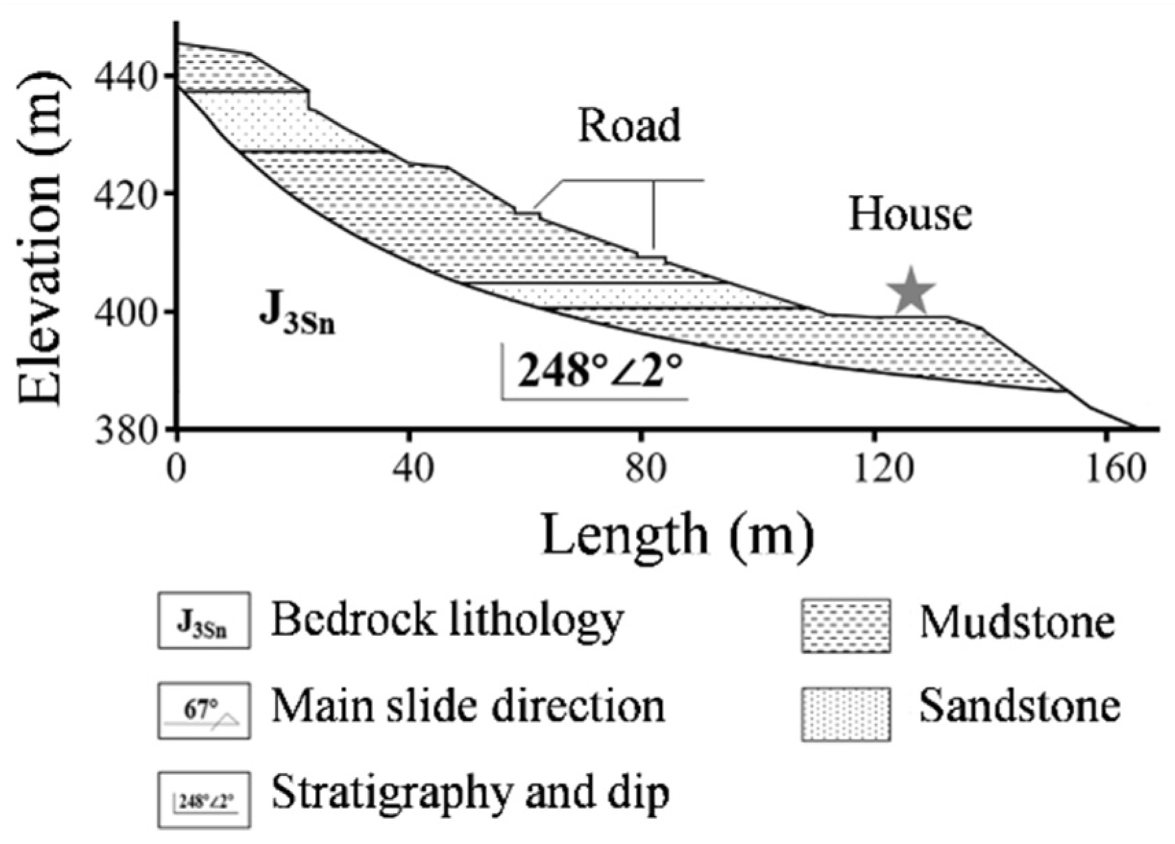
2.1. Introduction to Landslide in Tongnan District
2.2. Landslide Soil Parameters
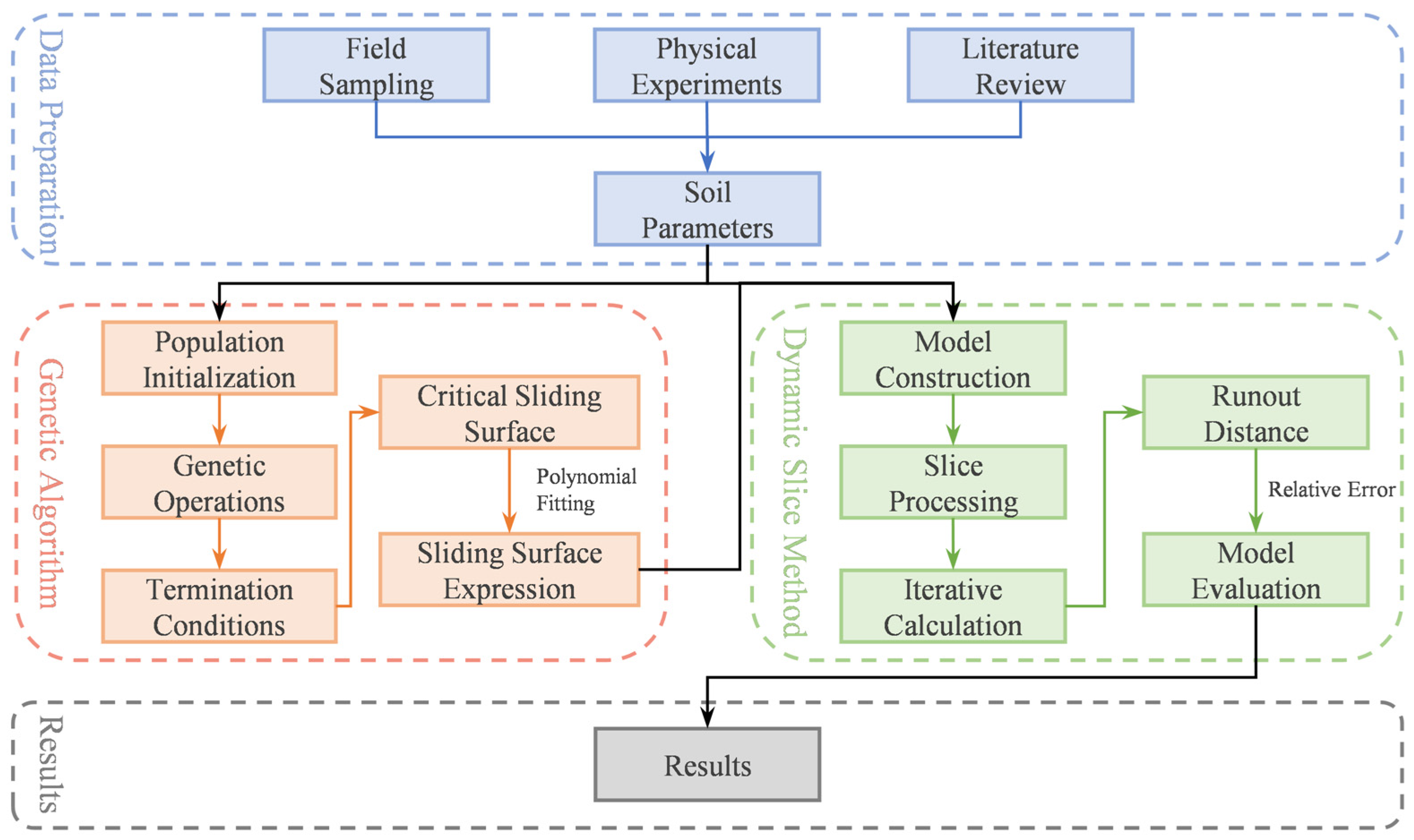
3. Methods
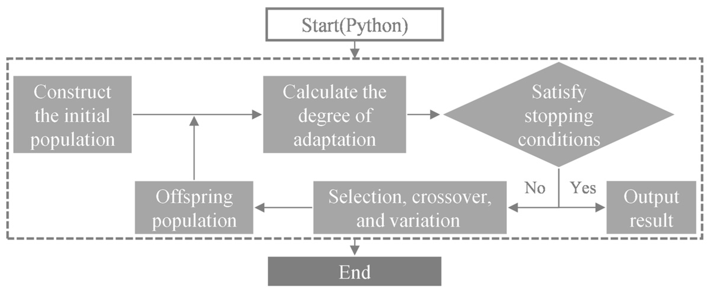
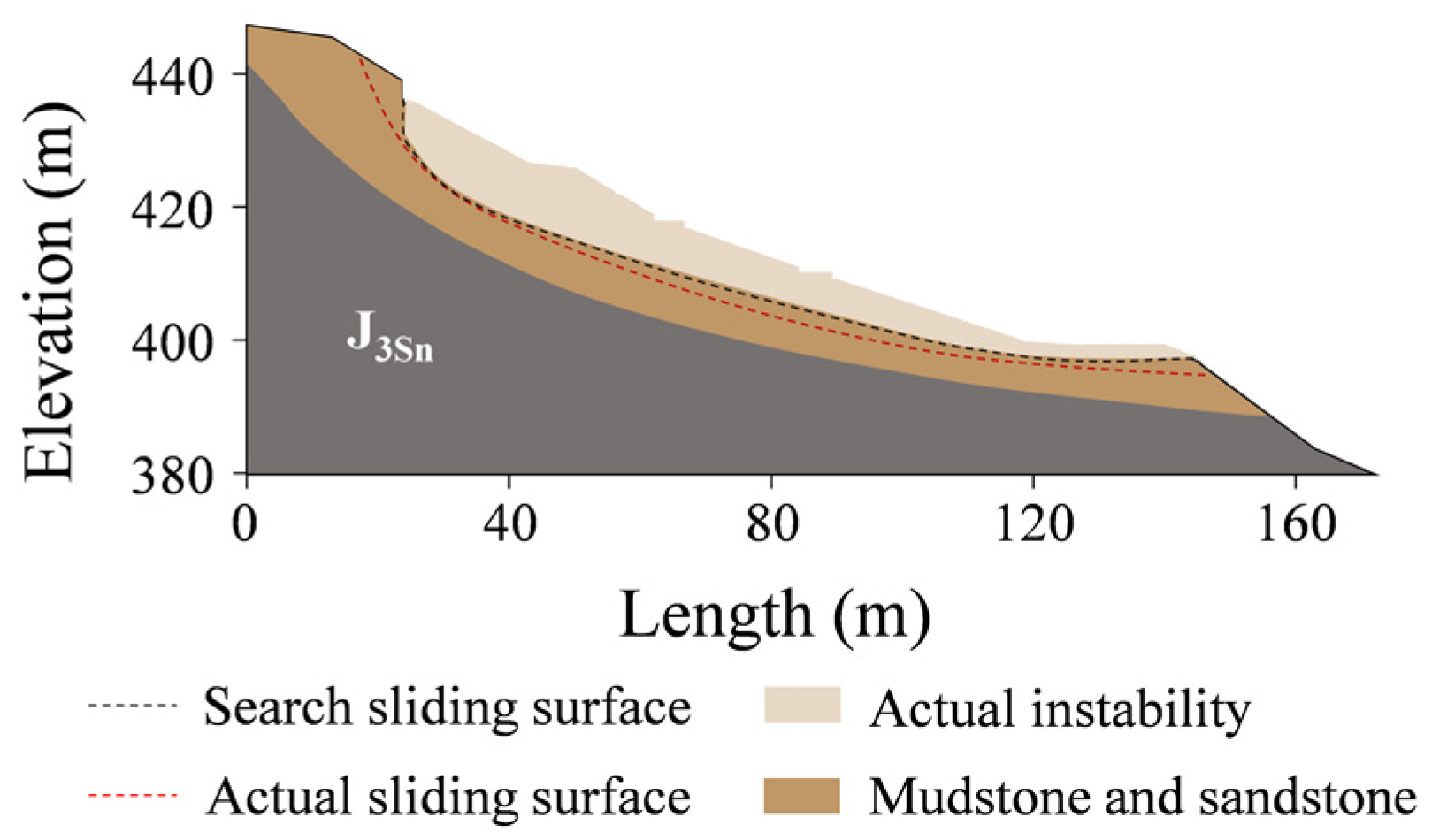
3.1. Hazardous Sliding Surface Search
3.1.1. Fitness Function
3.1.2. Genetic Algorithm Model
3.2. Calculation of Landslide Runout Distance
3.2.1. Dynamic Slicing Method Model
3.2.2. Model Assessment
4. Results
4.1. Hazardous Sliding Surface Search Result
4.2. Prediction of Landslide Runout Distance
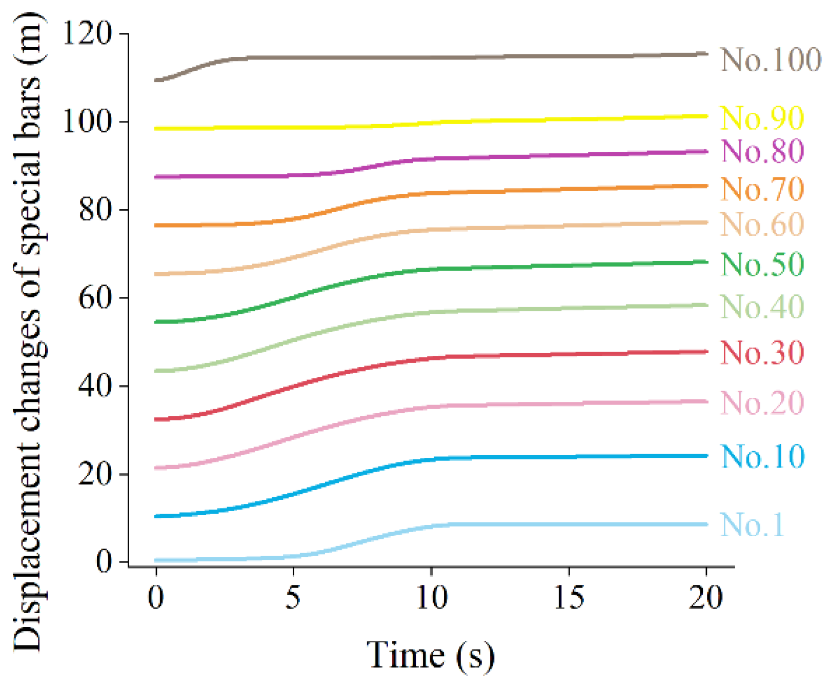
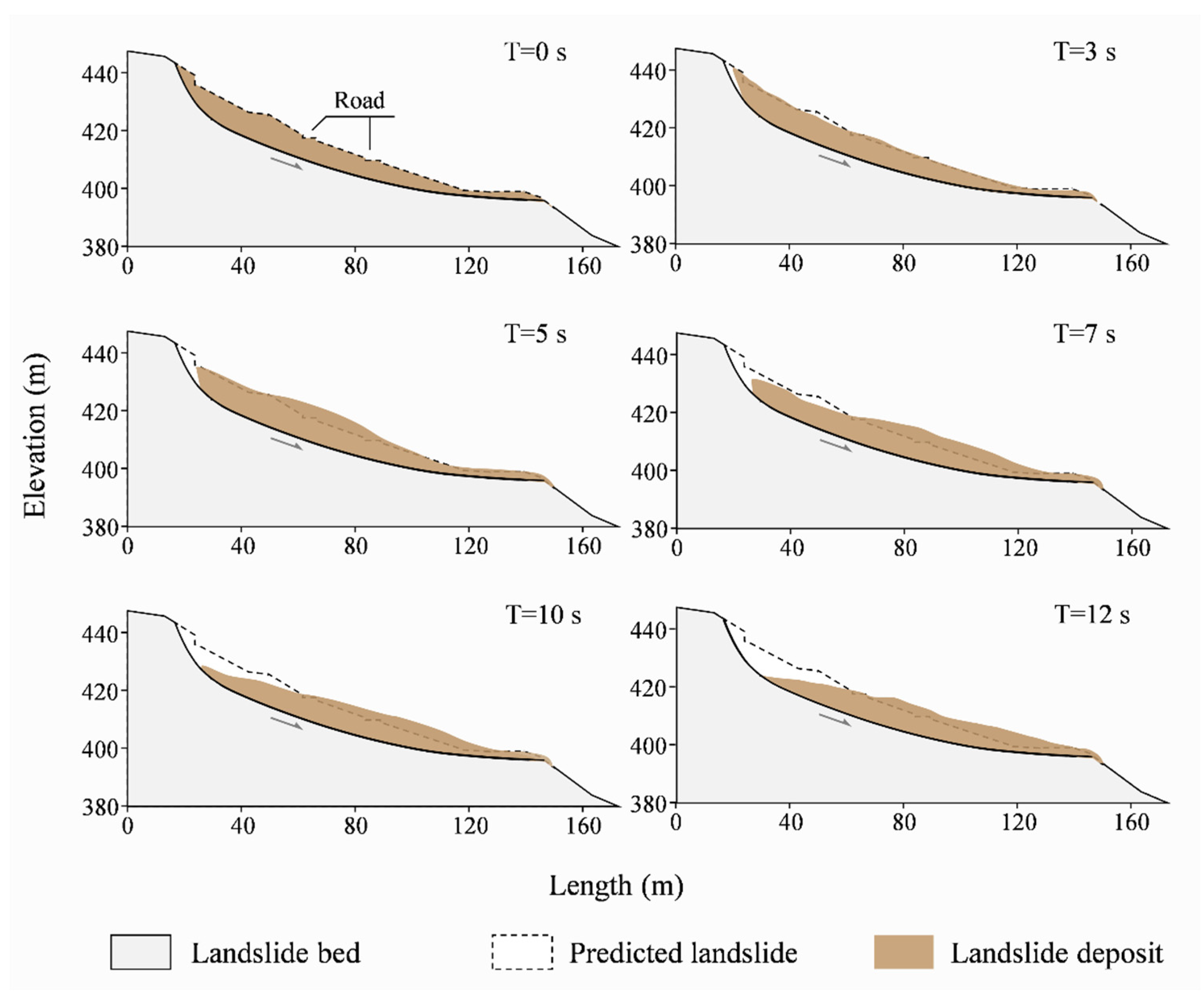
4.2.1. Landslide Runout Distance
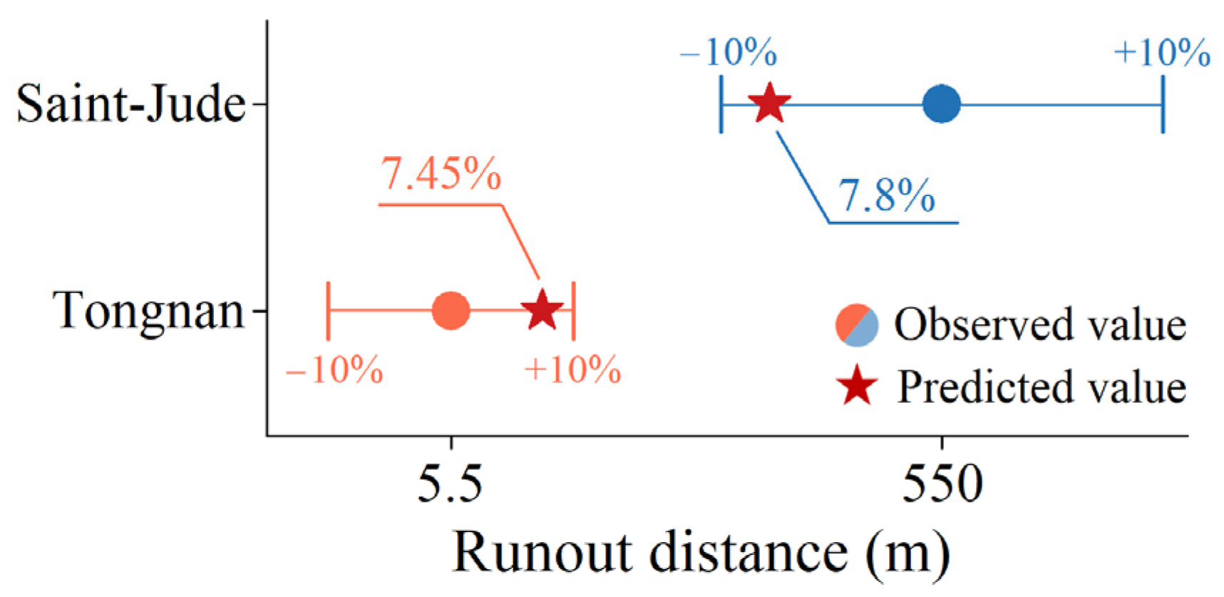
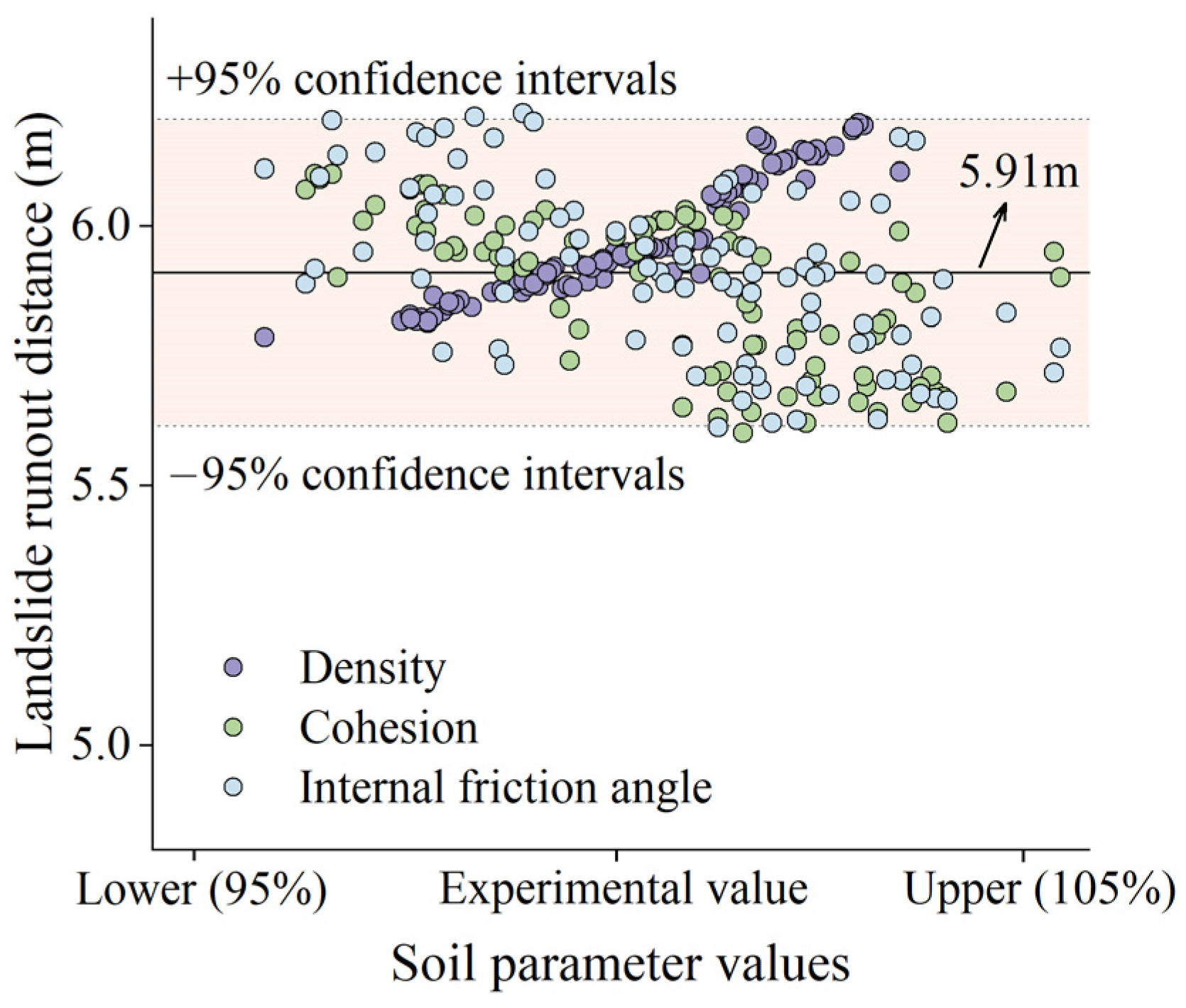
4.2.2. Results of Model Assessment
5. Discussion
5.1. Impact of Soil Moisture Content
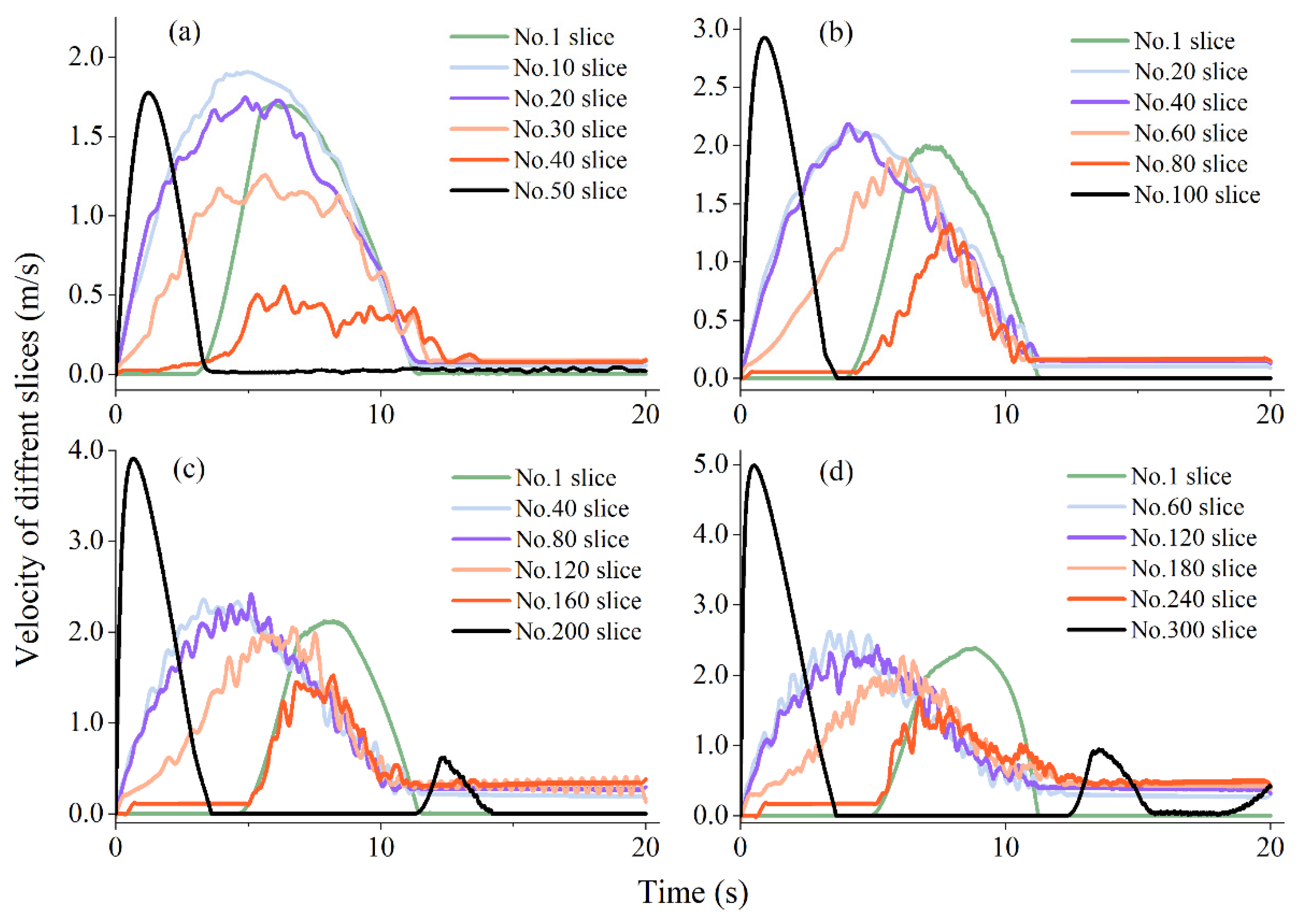
5.2. Impact of Number of Slices
5.3. Limitations and Prospects
6. Conclusions
Author Contributions
Funding
Data Availability Statement
Acknowledgments
Conflicts of Interest
References
- Ayesha, A.; Mohd, N.M.J.M.; Masa, G.; Shamsunnahar, K.; Ahmed, P.; Md, R. Landslide Disaster in Malaysia: An Overview. Int. J. Integr. Res. Dev. 2019, 8, 292–302. [Google Scholar] [CrossRef]
- Persichillo, M.G.; Bordoni, M.; Meisina, C. The role of land use changes in the distribution of shallow landslides. Sci. Total Environ. 2017, 574, 924–937. [Google Scholar] [CrossRef] [PubMed]
- Persichillo, M.G.; Bordoni, M.; Meisina, C.; Bartelletti, C.; Barsanti, M.; Giannecchini, R.; D’Amato Avanzi, G.; Galanti, Y.; Cevasco, A.; Brandolini, P.; et al. Shallow landslides susceptibility assessment in different environments. Geomat. Nat. Haz. Risk 2017, 8, 748–771. [Google Scholar] [CrossRef]
- Dong, Y.; Lan, Y.; Li, B.; Li, W. Study on deformation characteristics and early warning analysis of rainfall-type shallow soil landslide:case of orchard in Tongnan County, Chongqing City. Yangtze River 2020, 51, 97–101. [Google Scholar] [CrossRef]
- Qi, S.; Peng, S. Overview of the current status of landslide control and research at home and abroad. Saf. Environ. Eng. 2000, 3, 16–19. [Google Scholar]
- Iverson, R.M. Scaling and design of landslide and debris-flow experiments. Geomorphology 2015, 244, 9–20. [Google Scholar] [CrossRef]
- Schulz, W.H.; McKenna, J.P.; Kibler, J.D.; Biavati, G. Relations between hydrology and velocity of a continuously moving landslide-evidence of pore-pressure feedback regulating landslide motion? Landslides 2009, 6, 181–190. [Google Scholar] [CrossRef]
- Dang, V.-H.; Hoang, N.-D.; Nguyen, L.-M.; Bui, D.T.; Samui, P. A novel GIS-based random forest machine algorithm for the spatial prediction of shallow landslide susceptibility. Forests 2020, 11, 118. [Google Scholar] [CrossRef]
- Mohan, A.; Singh, A.K.; Kumar, B.; Dwivedi, R. Review on remote sensing methods for landslide detection using machine and deep learning. Trans. Emerg. Telecommun. Technol. 2021, 32, e3998. [Google Scholar] [CrossRef]
- Mohan, A.; Singh, A.K.; Kumar, B.; Dwivedi, R. An empirical–statistical model for predicting debris-flow runout zones in the Wenchuan earthquake area. Quatern. Int. 2010, 250, 63–73. [Google Scholar] [CrossRef]
- Li, B.; Gong, W.; Tang, H.; Zou, Z.; Bowa, V.M.; Juang, C.H. Probabilistic analysis of a discrete element modelling of the runout behavior of the Jiweishan landslide. Int. J. Numer. Anal. Met. 2021, 45, 1120–1138. [Google Scholar] [CrossRef]
- Gautam, P.; Michel, J. Method to estimate the initial landslide failure surface and volumes using grid points and spline curves in MATLAB. Landslides 2022, 19, 2997–3008. [Google Scholar] [CrossRef]
- Schäfer, M.; Teschauer, I. Numerical simulation of coupled fluid–solid problems. Comput. Methods Appl. Mech. Eng. 2001, 190, 3645–3667. [Google Scholar] [CrossRef]
- Zhang, L.; Fredlund, D.G.; Zhang, L.; Tang, W. Numerical study of soil conditions under which matric suction can be maintained. Can. Geotech. J. 2004, 41, 569–582. [Google Scholar] [CrossRef]
- Mak, J.; Chen, Y.; Sadek, M.A. Determining parameters of a discrete element model for soil–tool interaction. Soil Till. Res. 2012, 118, 117–122. [Google Scholar] [CrossRef]
- Persson, B.; Albohr, O.; Mancosu, F.; Peveri, V.; Samoilov, V.; Sivebaek, I. On the nature of the static friction, kinetic friction and creep. Wear 2003, 254, 835–851. [Google Scholar] [CrossRef]
- Ering, P.; Babu, G.L.S. Effect of spatial variability of earthquake ground motions on the reliability of road system. Soil Dyn. Earthq. Eng. 2020, 136, 106207. [Google Scholar] [CrossRef]
- Wu, F.; Fan, Y.; Liang, L.; Jin, J. Simulation Analysis of Landslide Motion Process Based on the Dynamic Slice Method. Adv. Eng. Sci. 2013, 45, 7–12. [Google Scholar] [CrossRef]
- Andersen, S.; Andersen, L. Modelling of landslides with the material-point method. Computat. Geosci. 2010, 14, 137–147. [Google Scholar] [CrossRef]
- Chen, Y.; Wang, S.; Wang, L.; Chen, Y.; Zhang, K.; Fan, Z.; Li, Q. A discrete element method for calculating saturated and unsaturated seepage in landslide soils and a case study. Landslides 2025, 1–17. [Google Scholar] [CrossRef]
- Orozco, A.F.; Steiner, M.; Katona, T.; Roser, N.; Moser, C.; Stumvoll, M.J.; Glade, T. Application of induced polarization imaging across different scales to understand surface and groundwater flow at the Hofermuehle landslide. Catena 2022, 219, 106612. [Google Scholar] [CrossRef]
- Chen, Y.; Fu, J.; Chen, J.; Ma, H.; Zhu, Z. Three-dimensional slope stability analysis based on irregular ellipsoid sliding surface. Heliyon 2024, 10, e35535. [Google Scholar] [CrossRef]
- Zhang, J.; Huang, H.W. Risk assessment of slope failure considering multiple slip surfaces. Comput. Geotech. 2016, 74, 188–195. [Google Scholar] [CrossRef]
- Wu, L.; Chen, H. Genetic Algorithm Analysis on Global Stability of Landslide and its Application. J. Chongqing Jiaotong Univ. Nat. Sci. 2009, 28, 907–910. [Google Scholar]
- Cao, B.; Wang, S.; Song, D.; Du, H.; Guangwei, L.; Zhiwei, Z. Landslide displacement prediction based on extreme learning machine optimized by ant colony algorithm. J. Water Resour. Water Eng. 2022, 33, 172–178. [Google Scholar] [CrossRef]
- Wang, C.; Fang, L.; Chang, D.; Huang, F. Back-analysis of a rainfall-induced landslide case history using deterministic and random limit equilibrium methods. Eng. Geol. 2023, 317, 107055. [Google Scholar] [CrossRef]
- Gordan, B.; Armaghani, D.J.; Hajihassani, M.; Monjezi, M. Prediction of seismic slope stability through combination of particle swarm optimization and neural network. Eng. Comput. 2016, 32, 85–97. [Google Scholar] [CrossRef]
- Chen, Z.; Zhu, L.; Lu, H.; Chen, S.; Zhu, F.; Liu, S.; Han, Y.; Xiong, G. Research on bearing fault diagnosis based on improved genetic algorithm and BP neural network. Sci. Rep. 2024, 14, 15527. [Google Scholar] [CrossRef]
- Liang, Y.; Leung, K. Genetic algorithm with adaptive elitist-population strategies for multimodal function optimization. Appl. Soft Comput. 2011, 11, 2017–2034. [Google Scholar] [CrossRef]
- Yao, W.; Li, C.; Zhan, H.; Zhang, H.; Chen, W. Probabilistic multi-objective optimization for landslide reinforcement with stabilizing piles in Zigui Basin of Three Gorges Reservoir region, China. Stoch. Environ. Res. Risk Assess. 2020, 34, 807–824. [Google Scholar] [CrossRef]
- Jiang, Q.; Liu, X.; Wei, W.; Zhou, C. Wedge stability analysis for rock slope and search for critical slip surfaces. Chin. J. Rock Mech. Eng. 2013, 32, 24–32. [Google Scholar]
- Dias, H.C.; Hölbling, D.; Grohmann, C.H. Rainfall-Induced Shallow Landslide Recognition and Transferability Using Object-Based Image Analysis in Brazil. Remote Sens 2023, 15, 5137. [Google Scholar] [CrossRef]
- Ran, Q.; Hong, Y.; Li, W.; Gao, J. A modelling study of rainfall-induced shallow landslide mechanisms under different rainfall characteristics. J. Hydrol. 2018, 563, 790–801. [Google Scholar] [CrossRef]
- Hou, C.; Zhang, T.; Sun, Z.; Dias, D.; Li, J. Discretization technique for stability analysis of complex slopes. Geomech. Eng. 2019, 17, 227–236. [Google Scholar] [CrossRef]
- Pastor, M.; Blanc, T.; Haddad, B.; Drempetic, V.; Morles, M.S.; Dutto, P.; Stickle, M.M.; Mira, P.; Merodo, J.A.F. Depth averaged models for fast landslide propagation: Mathematical, rheological and numerical aspects. Arch. Comput. Methods Eng. 2015, 22, 67–104. [Google Scholar] [CrossRef]
- He, F.; Tan, S.; Liu, H. Mechanism of rainfall induced landslides in Yunnan Province using multi-scale spatiotemporal analysis and remote sensing interpretation. Microprocess. Microsyst. 2022, 90, 104502. [Google Scholar] [CrossRef]
- Joo, A.; Ekart, A.; Neirotti, J.P. Genetic Algorithm for Discovery of Matrix Multiplication Methods. IEEE Trans. Evol. Comput. 2012, 16, 749–751. [Google Scholar] [CrossRef]
- Wang, C.L.; Ko, C.J.; Wong, H.K.; Pai, P.H.; Tai, Y.C. An Approach for Preliminary Landslide Scarp Assessment with Genetic Algorithm (GA). Water 2022, 14, 2400. [Google Scholar] [CrossRef]
- Van Quan, L.; Hanh, N.T.; Binh, H.T.T.; Toan, V.D.; Ngoc, D.T.; Lam, B.T. A bi-population Genetic algorithm based on multi-objective optimization for a relocation scheme with target coverage constraints in mobile wireless sensor networks. Expert Syst. Appl. 2023, 217, 119486. [Google Scholar] [CrossRef]
- Cavallaro, C.; Cutello, V.; Pavone, M.; Zito, F. Machine Learning and Genetic Algorithm: A case study on image reconstruction. Knowl. Based Syst. 2024, 284, 111194. [Google Scholar] [CrossRef]
- Ding, Z.; Tian, Y.-C.; Wang, Y.-G.; Zhang, W.; Yu, Z.-G. Progressive-fidelity computation of the genetic algorithm for energy-efficient virtual machine placement in cloud data centers. Appl. Soft Comput. 2023, 146, 110681. [Google Scholar] [CrossRef]
- Mahmood, A.; Al-Bayati, K.Y.; Szabolcsi, R. Comparison between Genetic Algorithm of Proportional–Integral–Derivative and Linear Quadratic Regulator Controllers, and Fuzzy Logic Controllers for Cruise Control System. World Electr. Veh. J. 2024, 15, 351. [Google Scholar] [CrossRef]
- Naidu, S.; Sajinkumar, K.; Oommen, T.; Anuja, V.; Samuel, R.A.; Muraleedharan, C. Early warning system for shallow landslides using rainfall threshold and slope stability analysis. Geosci. Front. 2017, 9, 1871–1882. [Google Scholar] [CrossRef]
- Liu, Y.; Gu, X. Skeleton-Network Reconfiguration Based on Topological Characteristics of Scale-Free Networks and Discrete Particle Swarm Optimization. IEEE Trans. Power Syst. 2007, 22, 1267–1274. [Google Scholar] [CrossRef]
- Meier, C.; Jaboyedoff, M.; Derron, M.; Gerber, C. A method to assess the probability of thickness and volume estimates of small and shallow initial landslide ruptures based on surface area. Landslides 2020, 17, 1–8. [Google Scholar] [CrossRef]
- Karpenko, Y.A.; Akay, A. A numerical model of friction between rough surfaces. Tribol. Int. 2001, 34, 531–545. [Google Scholar] [CrossRef]
- Mohan, S.; Vijayalakshmi, D.P. Genetic algorithm applications in water resources. ISH J. Hydraul. Eng. 2012, 15 (Suppl. 1), 97–128. [Google Scholar] [CrossRef]
- Eiben, A.E.; Smit, S.K. Parameter tuning for configuring and analyzing evolutionary algorithms. Swarm Evol. Comput. 2011, 1, 19–31. [Google Scholar] [CrossRef]
- Ali, R.; Mounir, G.; Moncef, T. Adaptive probabilities of crossover and mutation in genetic algorithm for solving stochastic vehicle routing problem. Int. J. Adv. Intell. Paradig. 2016, 8, 318–326. [Google Scholar] [CrossRef]
- Andrew, T.; Peter, R. Adapting operator settings in genetic algorithms. Evol. Comput. 1998, 6, 161–184. [Google Scholar] [CrossRef]
- Behnaz, K.; Naghi, Z.A.; Aliasghar, B.; Raziyeh, F. An open-source toolbox for investigating functional resilience in sewer networks based on global resilience analysis. Reliab. Eng. Syst. Safe 2022, 218, 108201. [Google Scholar] [CrossRef]
- Hai, H.; Meakin, P. Reply to comment by Dani Orand Teamrat Ghezzehei on “Computer simulation of two-phase immiscible fluid motion in unsaturated complex fractures using a volume of fluid method” by Hai Huang, Paul Meakin, and Moubin Liu. Water Resour. Res. 2006, 42, W07602. [Google Scholar] [CrossRef]
- George, D.L.; Iverson, R.M. A depth-averaged debris-flow model that includes the effects of evolving dilatancy. II. Numerical predictions and experimental tests. Proc. R. Soc. A: Math. Phys. Eng. Sci. 2014, 470, 1–31. [Google Scholar] [CrossRef]
- Ebert, E.E.; McBride, J.L. Verification of precipitation in weather systems: Determination of systematic errors. J. Hydrol. 2000, 239, 179–202. [Google Scholar] [CrossRef]
- Zhang, X.; Wang, L.; Krabbenhoft, K.; Tinti, S. A case study and implication: Particle finite element modelling of the 2010 Saint-Jude sensitive clay landslide. Landslides 2020, 17, 1117–1127. [Google Scholar] [CrossRef]
- Chiu, Y.; Chen, H.; Yeh, K. Investigation of the Influence of Rainfall Runoff on Shallow Landslides in Unsaturated Soil Using a Mathematical Model. Water 2019, 11, 1178. [Google Scholar] [CrossRef]
- Liang, Y.; Cui, S.; Pei, X.; Zhu, L.; Wang, H.; Yang, Q. Shear behavior of bedding fault material on the basal layer of DGB landslide. Sci. Rep. 2023, 13, 233. [Google Scholar] [CrossRef]
- Kererat, C. Effect of oil-contamination and water saturation on the bearing capacity and shear strength parameters of silty sandy soil. Eng. Geol. 2019, 257, 105138. [Google Scholar] [CrossRef]
- Ozbakan, N.; Evirgen, B. The effect of sodium polyacrylate gel on the properties of liquefiable sandy soil under seismic condition. J. Eng. Res. 2023, 11, 100006. [Google Scholar] [CrossRef]
- Jin, Y.; Zhu, B.; Yin, Z.; Zhang, D. Three-dimensional numerical analysis of the interaction of two crossing tunnels in soft clay. Undergr. Space 2019, 4, 310–327. [Google Scholar] [CrossRef]
- Yu, F.; Su, L. Experimental investigation of mobility and deposition characteristics of dry granular flow. Landslides 2021, 18, 1875–1887. [Google Scholar] [CrossRef]
- Liu, B.; Zhu, C.; Tang, C.-S.; Xie, Y.-H.; Yin, L.-Y.; Cheng, Q.; Shi, B. Bio-remediation of desiccation cracking in clayey soils through microbially induced calcite precipitation (MICP). Eng. Geol. 2020, 264, 105389. [Google Scholar] [CrossRef]
- John, S.M.; Marcelo, S.; Ingrid, T. Energy geotechnics: Advances in subsurface energy recovery, storage, exchange, and waste management. Comput. Geotech. 2016, 75, 244–256. [Google Scholar] [CrossRef]
- Peng, X.; Yu, P.; Chen, G.; Xia, M.; Zhang, Y. Development of a Coupled DDA-SPH Method and its Application to Dynamic Simulation of Landslides Involving Solid-Fluid Interaction. Rock Mech. Rock Eng. 2020, 53, 113–131. [Google Scholar] [CrossRef]
- Nouri, H.; Fakher, A.; Jones, C.J.F.P. Development of Horizontal Slice Method for seismic stability analysis of reinforced slopes and walls. Geotext. Geomembranes 2006, 24, 175–187. [Google Scholar] [CrossRef]
- Mehdipour, I.; Ghazavi, M.; Moayed, R.Z. Stability Analysis of Geocell-Reinforced Slopes Using the Limit Equilibrium Horizontal Slice Method. Int. J. Geomech. 2017, 17, 06017007. [Google Scholar] [CrossRef]
- Roy, C.J.; Oberkampf, W.L. A comprehensive framework for verification, validation, and uncertainty quantification in scientific computing. Comput. Methods Appl. Mech. Eng. 2011, 200, 2131–2144. [Google Scholar] [CrossRef]
- Celik, I.B.; Ghia, U.; Roache, P.J.; Freitas, C.J. Procedure for estimation and reporting of uncertainty due to discretization in CFD applications. J. Fluids Eng. 2008, 130, 078001. [Google Scholar] [CrossRef]


| Parameters | Saturation Density | Bed Friction Angle | Internal Friction Angle | Cohesion | Modulus of Elasticity | Poisson’s Ratio |
|---|---|---|---|---|---|---|
| (kg/m3) | (°) | (°) | (kPa) | (MPa) | (-) | |
| Values | 1900 | 16.5 | 22 | 26 | 8.92 | 0.35 |
| Moisture Content | Density (g/cm3) | Cohesion (kPa) | Internal Friction Angle (°) | R2 (Sliding Surface) | Runout Distance (m) | RE (%) |
|---|---|---|---|---|---|---|
| Initial state | 1.60 | 52 | 28 | 0.93 | 8.12 | 47.64 |
| Semi-saturation | 1.75 | 37 | 25 | 0.96 | 6.39 | 16.18 |
| Saturation | 1.90 | 26 | 22 | 0.98 | 5.91 | 7.45 |
| Number of Slices | 50 | 100 | 200 | 300 | ||
|---|---|---|---|---|---|---|
| Velocitymax (m/s) | 1.77 | 2.92 | 3.96 | 4.99 | ||
| MCV (-) | 0.69 | 1.11 | 1.15 | 1.29 | ||
| GCI (%) | 1.52 | 0.09 | 0.45 | |||
Disclaimer/Publisher’s Note: The statements, opinions and data contained in all publications are solely those of the individual author(s) and contributor(s) and not of MDPI and/or the editor(s). MDPI and/or the editor(s) disclaim responsibility for any injury to people or property resulting from any ideas, methods, instructions or products referred to in the content. |
© 2025 by the authors. Licensee MDPI, Basel, Switzerland. This article is an open access article distributed under the terms and conditions of the Creative Commons Attribution (CC BY) license (https://creativecommons.org/licenses/by/4.0/).
Share and Cite
Ren, W.; Zhou, W.; Hou, Z.; Tang, C. Prediction of Shallow Landslide Runout Distance Based on Genetic Algorithm and Dynamic Slicing Method. Water 2025, 17, 1293. https://doi.org/10.3390/w17091293
Ren W, Zhou W, Hou Z, Tang C. Prediction of Shallow Landslide Runout Distance Based on Genetic Algorithm and Dynamic Slicing Method. Water. 2025; 17(9):1293. https://doi.org/10.3390/w17091293
Chicago/Turabian StyleRen, Wenming, Wei Zhou, Zhixiao Hou, and Chuan Tang. 2025. "Prediction of Shallow Landslide Runout Distance Based on Genetic Algorithm and Dynamic Slicing Method" Water 17, no. 9: 1293. https://doi.org/10.3390/w17091293
APA StyleRen, W., Zhou, W., Hou, Z., & Tang, C. (2025). Prediction of Shallow Landslide Runout Distance Based on Genetic Algorithm and Dynamic Slicing Method. Water, 17(9), 1293. https://doi.org/10.3390/w17091293