Abstract
The present investigation utilized artificial neural networks (ANN) and gene expression programming (GEP) in comparison with the two-point method (TPM) to develop a generalized solution for predicting infiltrated water volume (∀Z) across various soil types under furrow conditions. This work assesses infiltration behavior with respect to experimental data from several temporal contexts. Data distribution and model performance are evaluated via descriptive statistics and correlation tests. Artificial intelligence (AI) models (ANN and GEP) trained and evaluated utilizing input variables—inflow rate (); furrow length (); waterfront advance time at the end of the furrow (); infiltration opportunity time (); and cross-sectional area of the inflow () are compared with TPM performance. More precisely and consistently than the water advance power function, AI-based algorithms hope to be invading water volume. Statistical analysis shows that ANN and GEP have lower error metrics, increased generalizability, and better representation of complex infiltration dynamics. The determination coefficient (R2) of ANN data produced 98.1% for testing and 97.8% for validation, while TPM showed accuracy reductions of 2.5% and 4.6%, respectively. On the other side, the R2 of GEP produced 95.7% for testing and 96.1% for validation, while TPM showed accuracy reductions of 0.7% and 3%, respectively. During ANN model computation, TPMs root mean square error (RMSE) of 0.0135 m3/m exceeded all mean values. Errors within 10% relative deviation were displayed using the ANN model . Particularly, ANN and GEP, the study revealed that AI techniques predict furrow irrigation penetration of water volume better than the water advance power function. These models advance soil and furrow adaptation, extrapolation, and accuracy. Results show that AI-driven modeling may maximize hydrological assessments and irrigation control.
1. Introduction
Soil infiltration behavior is crucial to surface irrigation system evaluation and design. For surface irrigation model creation, most designers must determine soil infiltration parameters. Infiltration patterns vary over a field. Seasonal agricultural practices affect infiltration patterns []. Moreover, Liu, Cui [] stated that the infiltration process is influenced by the availability of water and the permeability of the soil, which determines the volume of water that penetrates the soil profile from surface runoff. The behavior of soil water infiltration is regulated by both energy and mass transport mechanisms, with the initial soil moisture content significantly contributing to the formation of mass and energy gradients. An increase in soil moisture reduces the hydraulic gradient, thereby diminishing the driving force that facilitates water infiltration into the soil. Consequently, soil infiltrability can be viewed as a property of the soil that is contingent upon the initial profile of soil water content. Although machine learning techniques have demonstrated potential in precise forecasting and tracking of soil moisture levels, they frequently encounter challenges related to overfitting, inadequate generalization, and physical inconsistencies due to restricted and noisy subsurface information. These drawbacks could be mitigated through the use of specialized models like the Physics-Informed Neural Networks (PINN-SM) model [] and the Physics-Informed Machine Learning (PIML-SM) [] model, which have been shown to successfully connect data-driven approaches with physical insights in environmental modeling scenarios.
Furrow irrigation depends on how surface soil materials react to water, how moisture spreads inside the soil before irrigation starts, how water shifts across the zone, and how deep the water flows, while considering design elements like furrow measurement, slope ratios, geometrics, and water velocity [,]. Several empirical surface irrigation infiltration computation methods based on time evolution have been developed. Many infiltration models lack physical principles since they apply the Horton, Kostiakov, and Modified Kostiakov equations [,]. Using the hydrodynamic system, zero inertia (ZI), kinematic wave (KW), and volume balance (VB), several furrow irrigation assessment and design models have been constructed []. VB or ZI assessments are used in most research []. VB simple model precision compares to ZI complex model accuracy in speed and accuracy. For practical and routine tasks, engineers use basic models. However, the technological workforce and high financial costs due to long execution periods limit the use of sophisticated models in surface irrigation design and evaluation; therefore, VB is preferred [].
In VB theory, Elliott and Walker [] devised a well-known two-point strategy to choose two data points for the advanced phase throughout the midfield and lower field. Surface irrigation commonly uses the two-point approach to estimate empirical infiltration parameters since it involves a few data points and simple arithmetic. Using two advanced phase sites at the mid-distance and downstream ends of the field, the technique presumes a power function advance. Examining the two-point approach (TPM), Bautista, Clemmens [] recommended changes. The researchers noted that, though it is straightforward, the method can generate false findings. They suggested including readily obtained data in assessments to raise the performance of the approach. Bautista, Strelkoff [] investigated volume-balance model infiltration calculation errors. The study found TPM issues and suggested fixes to improve infiltration parameter estimation. In addition, Khatri and Smith [] examined surface irrigation simulation models, including the TPM. TPM is helpful in some situations, although it may not be as precise as more complex models. These studies demonstrate that while the TPM is good for its simplicity and low data requirements, engineers should know its limits. For surface irrigation infiltration parameter determination, more complex approaches may be needed, especially where precision is required.
Panahi, Seyedzadeh [] used the TPM to estimate border irrigation infiltration parameters during midpoint selection. The researchers ran two tests using the average advance time location, or mean infiltration opportunity time, as the midpoint. Researchers found that this powerful advanced equation calibration midpoint predicted advances in phase duration with 11.3% relative inaccuracy. New two-point and one-point furrow irrigation infiltration parameter estimation methods were developed by Kargas and Mindrinos []. The study assumed that water penetration into soil and furrow front movement follow two parameter-type equations. New assessment methodologies streamlined data gathering to improve infiltration measurement precision. Because it provides practical and successful solutions in many irrigation settings, the TPM remains significant for analyzing surface irrigation in various irrigation environments. Several research groups have employed VB approaches to examine surface irrigation system infiltration patterns. Simplified VB methods like one-point, two-point, and furrow infiltrometer, and advanced ones, require little data and execution. These approaches can generate measurement errors when field conditions differ from the infiltration equations. Maghferati, Chari [], studied surface irrigation volume-balance methods. Research produced a volume-balance TPM for the Philip infiltration equation that was then compared with the other seven approaches.
Hence, accurate prediction of the infiltration process using robust tools is one of the most important tasks in hydrological science. Panahi, Khosravi [] employed a convolutional neural network (CNN) in conjunction with gray wolf optimization (GWO), a genetic algorithm (GA), and independent component analysis (ICA) to predict cumulative infiltration and infiltration rates. A total of 154 raw datasets were gathered, which included variables such as measurement time, percentages of sand, clay, and silt, bulk density, soil moisture content, infiltration rate, and cumulative infiltration through field surveys. The findings indicated that the timing of measurements is critical for predicting cumulative infiltration, whereas soil properties, particularly silt content, play a more significant role in predicting infiltration rates. This suggests that in the study area, the silt parameter, which is a key constituent, can more effectively govern infiltration processes. Furthermore, it was observed that soil moisture content and bulk density had limited effectiveness in this study, as these two factors showed minimal variability across the area. The results demonstrated that CNN algorithms exhibit high performance, and the application of a metaheuristic algorithm improved the performance of a standalone CNN by 7% to 28%. Additionally, the CNN-GWO algorithm outperformed the other approaches, followed by CNN-ICA, CNN-GA, and CNN, in both cumulative infiltration and infiltration rate predictions.
Agricultural engineers have increasingly relied on artificial neural networks (ANN) and gene expression programming (GEP) as main soft computing technologies for irrigation system development in recent years. Wang [], applied the Enhanced Genetic Algorithm—Backpropagation Neural Network (EGA-BPNN) model to innovative agriculture systems to create an intelligent field irrigation warning system that accurately forecasts irrigation flow and empowers farmers with science-based decisions. Abdulsalam, Lawal [], examined how GEP and ANN can estimate hydrochar physicochemical parameters. Research showed that these models may detect complicated agricultural relational patterns in data analysis. Raza, Vishwakarma [], determined reference evapotranspiration (ETref) using GEP with little meteorological data. ETref forecasts from Generalized Evolution Programming are useful for irrigation preparation with limited data. ANN and GEP methods in agricultural engineering are being used to improve irrigation system metrics.
ANNs have become somewhat well-known for soil water infiltration modeling as they fit the Kostiakov model parameters. Al-Janobi, Aboukarima [], used ANNs to simulate Kostiakov infiltration equation parameters in clay soil with traditional tillage. The simulation rates matched observed rates during different infiltration periods. ANNs outperformed Philip and Green-Ampt standard equations in cumulative infiltration studies. El Marazky, Aboukarima [], examined how typical clayland farming affected water seepage. ANN research yielded simulations that matched infiltration rate trends. ANNs mimic soil infiltration processes well, a key tool for irrigation practice optimization.
Numerous models exist for simulating water movement; however, many of these models rely on overly simplified estimates of infiltration, which often lack a solid empirical foundation and fail to accurately represent actual field conditions. Despite this limitation, the practical application of these infiltration models has not been thoroughly addressed. Recognizing these limitations and challenges, the present work aims to develop a generalized solution for infiltration that can be effectively applied across various soil types and furrow conditions by (1) building prediction models for the volume of infiltrated water in a furrow using ANN and GEP and (2) comparing the infiltration data outputs from the ANN, GEP, and TPM models.
2. Materials and Methods
2.1. Data Collection
The database utilized for developing the artificial neural network (ANN) alongside the Gene Expression Programming (GEP) model was sourced from existing literature. A total of 159 data points were aggregated from six different studies. Valiantzas, Aggelides [], Alvarez [], Holzapfel, Jara [], Playán, Rodr ı’ guez [], Mateos and Oyonarte [], and Sepaskhah and Shaabani []. These studies were conducted in various locations with differing soil types and furrow geometries, and multiple discharge rates were evaluated at each site. Two distinct field experiments were carried out. The first experiment focused on furrow infiltration using an infiltrometer to estimate the infiltration parameters based on the empirical Kostiakov equation. The second experiment involved measurements related to land leveling conditions, furrow discharges, furrow cross-sections, advance time, recession time, and hydraulic roughness. Measurement stations were established at specific distances from the furrow head. During the advancing phase, as the inflowing water entered the furrows and reached each station, the time taken to reach each station, water depth, surface water width, flow cross-section, and wetted perimeter were recorded. Upon cessation of the inflow, the time it took for the water to recede at each station was noted to determine the recession times. The infiltration opportunity time along the furrow at each station was then calculated as the time difference between when the water disappeared and when it first started to advance at the same location along the furrow. Both experiments were conducted in the same field and under similar conditions. The infiltration parameters derived from the first experiment were applied to estimate the volume of furrow-infiltrated water in the second experiment. Table 1 provides details of the sites and the values of the process variables and outputs.

Table 1.
Experimental collected data.
The datasets utilized for the development of the ANN and GEP models were compiled to include several input variables: inflow rate; represents governing water delivery dynamics, furrow length ; for defining the spatial scale of irrigation, waterfront advance time at furrow terminus ; to characterize temporal progression, infiltration opportunity time ; which reflecting cumulative exposure duration, the cross-sectional area of inflow ; that measuring the infiltrated exposed surface area, The output variable is infiltrated water volume . The meticulously selected dataset is an appropriate base for building and testing ANN and GEP models, boosting predictive capabilities for furrow irrigation investigations.
2.2. Artificial Neural Network (ANN)
ANNs model intricate hydrological processes rather well. Three layers—input; hidden; and output—define a typical feedforward ANN. External data for the hidden levels is received and encoded in the input layer. Using weighted modifications and nonlinear activation patterns, several connected neurons in these deep layers extract and examine data properties. The output layer at last generates from processed data the predictions or classifications of the network. Information flow and learning of the ANN depend on the neurons of every layer. By weighted interactions, such neurons preserve the gained knowledge and bias values of the network []. Applying activation functions to their weighted input sums helps neurons to acquire nonlinearity. Working with both positive and negative inputs, hyperbolic tangent (tanh) is an activation function returning outputs between −1 and 1 []. During training, back-propagation automatically modulates connection weights to match network predictions to output data. To reduce error by direction-based modification, gradient descent computes loss function derivatives for weights []. Hyperparameters, including learning rate, momentum factor, hidden layer nodes, and total hidden layers, must be exactly changed if successful ANN models are to be built. Up until the model balances accuracy and system complexity, constant testing maximizes these values. Normalizing techniques help training by allowing data to be adapted to match a 15% to 85% range. After several training cycles, the network provides rudimentary forecasts and approaches the error limit. The schematic of the ANN modeling is displayed in Figure 1.
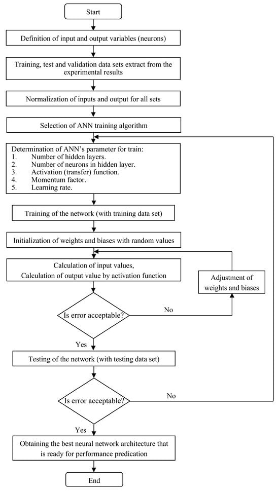
Figure 1.
Schematic illustration of the ANN technique.
The ANN structure was calculated by the Qnet2000 software for estimation. The first layer contained neurons matching the number of influential factors, which included , as illustrated in Figure 2. Within the output layer, a solitary neuron was designated to represent the variable . The available data (159 data points) was distributed randomly into a training set (70% of the dataset), a testing set (20%), and a validation set (10%). The training and testing sets, therefore, contain 112 and 31 data points, respectively, while the validation set has the remaining 16 data points. A data partitioning approach improved the ANNs reliable performance and estimation capabilities for predicting .
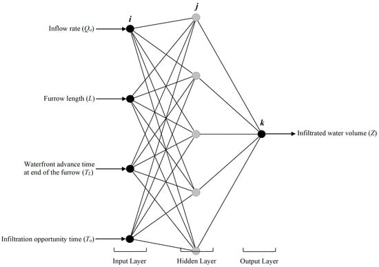
Figure 2.
The ANNs architecture employed for forecasting infiltrated water volume.
2.3. Gene Expression Programming (GEP)
Genetic programming (GP), proposed by Koza [], has been an efficient computational method for generating data-based models for decades. GEP is an important development in GP by uniting significant elements from both GAs and GP, as explained by Ferreira []. GEP inherits its representation from genetic algorithms using fixed-length linear strings called genes or chromosomes. The linear genetic structures become expression trees of diverse shapes and sizes under genetic programming []. To define all developed expressions, GEP hierarchical structures use mathematical operations (functions) and input variables or constants (terminals). Genetic procedures, including mutation, recombination, and transposition, are changeable programming. A predefined fitness function examines candidate solutions over numerous evaluation cycles to identify the best solution and find the best mathematical model.
Figure 3 shows GEP in action. Five basic GEP steps solve problems. The first step defines endpoints and functions for chromosomes. The terminal set has five independent variables: . The function set includes basic arithmetic operators (addition, subtraction, multiplication, and division) and essential mathematical functions like H, ln(x), log(x), exponential, base-10 exponential, and power functions. Ferreira [] states that the second phase is assessing program fitness. Research determines gene number and head length to establish chromosomal architecture numerical parameters and qualitative variable values. A chromosome with three genes and seven unit-length heads is tested in this work. In the fourth stage, a linking function that additively integrates genes is chosen to connect these program fragments. Mutation, inversion, transposition, and recombination rates were chosen for this research at the fifth step of genetic operator rate selection. The GEP model was created using GeneXproTools 5.0 []. GEP approach data subsets matched ANN analysis data subsets.
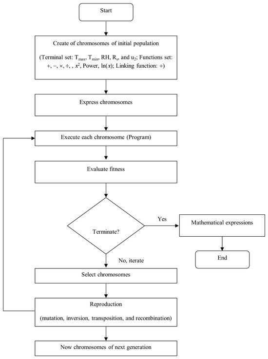
Figure 3.
Schematic flowchart representing the fundamental structure of GEP algorithms.
2.4. Two-Point Method (TPM)
The two-point method (TPM) was originally introduced by Elliott and Walker []. TPM uses the volume balance equation and the midpoint and endpoint of a furrow on the advance curve to estimate infiltration parameters [,] that are as follows (Equation (1)). This method has been widely used due to its simplicity and limited data requirements.
where is the advance distance along the field (m), and β are fitting parameters from two measured points of the advance curve (dimensionless), and is advance time (min).
This method was designed to determine the modified Kostiakov equation infiltration parameters for furrow irrigation. This method is mathematically formulated in Equation (2).
In this expression, denotes the cumulative infiltration measured in (cubic meters per meter). The empirical coefficients (with units of cubic meters per meter per minute) and (dimensionless) are determined through calibration. The parameter represents the basic infiltration rate, also expressed in cubic meters per meter per minute (cubic meters per meter), while signifies the infiltration opportunity time, measured in minutes.
Integrating Equations (1) and (2) yields Equation (3), the volume balance equation.
where and are surface and subsurface, respectively, water profile shape factors.
The value of typically ranges from 0.7 to 0.9, assuming a constant value during advancement []. Walker and Skogerboe [] proposed = 0.77.
Kiefer Jr [] developed an equation for by comparing Equation (1) to Elliott and Walker [] fitting methods (Equation (4)).
To solve k and a simultaneously, use Equation (3) at two places on the advance curve: the center and end of the furrow (Equations (5) and (6)).
Field measurements determined the basic infiltration rate , using the inflow-outflow approach []. To determine soil infiltration, calculate the difference between recorded input and outflow rates during irrigation episodes. This strategy is represented mathematically in Equation (7).
where is outflow from the end of the furrow (m3/min).
2.5. Statistical Evaluation Criteria
The coefficient of determination (R2), root mean square error (RMSE), efficiency coefficient (E), mean absolute error (MAE), model performance’s overall index (OI), and residual mass coefficient (CRM) were used to measure goods fit for the ANN, GEP, and TPM, as follows (Equations (8)–(13)):
where is observed value of ; is calculated value of by ANN, GEP, and TPM; n is number of observations; is averaged observed values of ; and is averaged calculated values of by ANN, GEP, and TPM.
The observed-expected value relationship is calculated using R2. Excellent model performance is indicated by R2 values nearing 100%. The model assessment process is more informative with RMSE because it communicates mistakes in variable units []. Higher model accuracy occurs when RMSE decreases. A model is effective when the E value is 1, but it can potentially be harmful. The MAE difference estimates the difference between expected and actual data points using the average value. Low MAE indicates good model performance.
3. Results and Discussion
3.1. Data Acquisition and Statistical Analysis of Infiltration Parameters
The acquisition of data occurred under different time settings. The evaluation spans up to 1000 min through time intervals of 100 min. Several cases failed to exceed 500 min, while others did not reach that limit. The results show difficulties in describing individual cases, as shown in Table 1. Environmental factors and soil types did not affect the water infiltrated volume, starting at low entry levels and growing gradually until a stable state. The infiltration rate exhibited the opposite behavior compared to the infiltration rate by moving from an initial high point to a quick reduction and reaching a point of stability. Two possible reasons for these changes include transitioning between unsaturated and saturated states of soil or soil sealing development. A specific soil type reacts to rain by forming crusts that might cause reduced infiltration rates.
The statistical analysis in Table 2 contains data for parameters. The table displays as measurement parameters for identifying minimum, maximum, mean, standard deviation, kurtosis, and skewness. The minimum and maximum values of the variable derived from the training dataset are fully encapsulated within the range of values observed in the testing set. This alignment indicates a consistent statistical distribution between the two datasets, as the extremes of (training) do not exceed the boundaries defined by (testing). Such coherence in data variability underscores the robustness of the dataset partitioning, ensuring that the model’s training regime remains representative of the testing conditions. This overlap mitigates risks of extrapolation errors and reinforces the generalizability of predictive outcomes, as the model is not exposed to out-of-range values during validation. The standard deviation of the variable shows similar minimal values for training and testing data samples. The training data shows elevated values for parameters, yet testing data demonstrates low values of .
Table 2.
Descriptive statistical parameters of training and testing datasets for model development variables.
Model development requires selecting appropriate inputs that provide the best understanding of the analyzed problem. The evaluation method is based on cross-correlation analysis between input variables and output variable is widely used and reported in Table 3. The authors excluded correlation values below 10% from further analysis. Table 3 indicates that all inputs have an R-value exceeding 10%. The analysis utilized as input values for prediction.
Table 3.
Correlation matrix illustrating relationships between input parameters and the output variable.
3.2. Representation of Infiltrated Water Volume
Time of opportunity displayed different outcomes through the collected data. The evaluation duration reached 1000 min, while the measurements occurred every 100 min. The measurements for some instances did not exceed 500 min during the evaluation period. A problem emerged when showcasing case-specific features within these data tables (Table 1). Regardless of differing soil types and environmental factors, the volume of water that infiltrated experienced a consistent pattern from low levels to increasing water intake and stabilized eventually. The infiltration rates followed an opposite pattern throughout the data collection process. At the beginning of the process, the penetration rate showed high values before declining to reach an almost steady-state level. The soil transition from an unsaturated state to saturation or the formation of surface crusts explains this observed phenomenon. The particular characteristics of the soil might contribute to lowering the infiltration rate during cases when moisture causes the soil to form a crust.
These experimental data require numerous equations that equal the number of tests performed for any description. The representation of these points using a universal equation appears complicated because of their abundance. The two-point method (TPM) represents a possible approach to complete this work. The required input data must exceed the inflow rate ; represents governing water delivery dynamics, furrow length ; for defining the spatial scale of irrigation, the waterfront advance time at the furrow terminus ; to characterize temporal progression, infiltration opportunity time ; which reflects cumulative exposure duration, the cross-sectional area of inflow ; that measures the infiltrated exposed surface area. Furthermore, supplementary parameters—Manning’s roughness coefficient; longitudinal slope; and furrow geometry—collectively influence hydraulic resistance and flow distribution. Collecting and processing this extensive dataset can be time-consuming and labor-intensive. In contrast, the ANN model demonstrates enhanced computational efficiency by streamlining input requirements. Through its ability to discern nonlinear relationships and latent patterns, the ANN architecture reduces dependency on exhaustive variable sets while maintaining high predictive accuracy. This parsimony not only minimizes data preprocessing burdens but also accelerates computational processing times, as elaborated in subsequent analyses. The ANNs superior performance stems from its adaptive learning mechanisms, which mitigate redundancies inherent in conventional empirical methods, thereby optimizing resource allocation in both theoretical and applied irrigation studies.
3.3. Artificial Neural Network (ANN) Architecture
Decision-making for ANN structure requires examining how many hidden layers to use, determining the number of neurons included in each layer, and the activation function per inter-layer connection. The evaluation of a perfect ANN architecture requires time-consuming individual testing because this methodology lacks predictive methods. The evaluation process allows researchers to test different architectural structures empirically, which leads to identifying the optimal model design for each task []. The research’s selection method followed three stages using the information presented in Table 4. Model performance depends heavily on variable selection during ANN modeling since it represents a fundamental process within this methodology. At the beginning of the study, researchers used the ANN 5-2-1 neural system with five inputs, two hidden, and one output neuron to evaluate the importance of the input variable . The variable accounted for only 4.53% and 6.68% of the output results from the ANN model when using sigmoid and hyperbolic tangent (tanh) activation functions, yet remained less important than other model variables. Statistical multiple linear regression results confirmed (p < 0.05) the significance of all variables apart from . This study removed the variable from further research due to its weak impact on the outcome. The refined ANN model employed architecture 4-j-1 to include the variables . Valid ANN architecture selection requires stepwise testing and validation because it ensures the model effectively captures original data patterns without compromising efficiency or economy.
Table 4.
Statistical evaluation of ANN model performance based on varying concealed layer nodes, transfer functions, and iteration counts.
The statistical indicators in Table 4 show slight improvement when the ANN (4-2-1) operates without variable at its second analysis stage. The change to a determination coefficient (R2) value of 93.1%, along with a reduction of about 22% in maximum error and a 4% reduction in the SD, proves successful. The accuracy levels of the network remained unchanged when the iteration amount increased from 5000 to 100,000 during this construction period, regardless of the choice of function. Network performance gains significantly when the j value is raised from two to three (4-3-1) while implementing the tanh function. The application of the hyperbolic tangent (tanh) activation function resulted in the most optimal network performance across 100,000 iterations. This optimization was evidenced by a significant improvement in the determination coefficient (R2), which reached an impressive 98.2%. Additionally, the maximum error exhibited a notable reduction, decreasing from 0.0431 m3/m (when j = 2) to 0.0298 m3/m. Moreover, the standard deviation of errors was reduced by half when compared to the values obtained from the 4-2-1 network configuration. The sigmoid function achieved a 97.9% R2 value while generating maximum error results at 0.031 m3/m and SD at 0.87%. These findings highlight the tanh function’s effectiveness in enhancing the network’s predictive accuracy and stability.
The training process of ANN underwent significant improvement after j was raised from three to five through the implementation of the tanh function in the third stage of the study, as Table 4 demonstrates both an R2 of 98.5% with minimum and maximum error at 0.027 m3/m and the lowest SD value of 0.74% achieved at 100,000 number of iterations. When the j value exceeds five, ANNs performance degradation begins.
The ANN architecture 4-5-1 in Figure 2 proves the most suitable because it produces the most accurate predictions with minimum errors. Table 5 presents the connection weight parameters and bias values utilized in the tanh activation function within the proposed ANN model. These parameters play a crucial role in optimizing the network’s ability to accurately simulate . The mathematical formulations governing these computations are provided in Equations (14) and (15), which define the weight distributions and bias adjustments essential for enhancing the predictive performance of the ANN model.
where:
is output variable ; is biases in the output layer; is number of nods; is weights between hidden and output layers; is number of output node; is biases in the hidden layer; is number of input nodes; is weights between input and hidden layers; and is input variables .
Table 5.
Connection weights (W) and biases (B) values obtained for the ANN model.
Table 5.
Connection weights (W) and biases (B) values obtained for the ANN model.
| (W1)ji between input and concealed layers, and (B1)j for concealed layer | |||||
| (W1)1i | (W1)2i | (W1)3i | (W1)4i | (W1)5i | |
| (W1)j1 | −0.511 | 1.307 | −0.832 | 0.077 | −0.550 |
| (W1)j2 | 0.703 | −1.435 | 2.113 | −3.369 | 3.089 |
| (W1)j3 | 0.933 | −0.545 | −0.872 | −2.603 | −0.254 |
| (W1)j4 | 5.999 | −0.011 | −2.154 | 2.267 | 0.572 |
| (B1)j | −0.867 | 1.295 | 0.753 | 1.372 | −0.416 |
| (W2)kj between concealed and output layers, and (B2)k for the output layer | |||||
| (W2)k1 | (W2)k2 | (W2)k3 | (W2)k4 | (W2)k5 | |
| (W2)1j | 3.456 | 2.125 | −2.396 | −2.102 | −3.231 |
| (B2)k | 0.238 | ||||
3.4. Performance Evaluation and Optimization of the ANN Model
Figure 4 illustrates the degree of fitting between the trained ANN model’s predictions and the observed values of infiltrated water volume . The figure highlights a strong agreement between the predicted and measured data, as evidenced by the clustering of points closely around the 1:1 line. This suggests that the ANN model effectively captures the underlying patterns governing the infiltration process. Moreover, the network demonstrates its capability to accurately predict values across a broad range of process variables, as detailed in Table 1. To assess the ANN model’s predictive performance, a comprehensive statistical evaluation was conducted by comparing the predicted and observed values. The developed ANN model achieved an R2 of 98.5%, a root mean square error (RMSE) of 0.005 m3/m, an efficiency coefficient (E) of 98.7%, an overall index of performance (OI) of 98.5%, and a coefficient of residual mass (CRM) of 0.4%, as presented in Table 6. The R2, E, and OI values being very close to one indicate a highly accurate predictive capability, while the RMSE and CRM values approaching zero further confirm the model’s precision. These findings establish an excellent agreement between the ANN model’s predictions and the experimental data, with minimal deviations observed between the two. Furthermore, the results suggest that furrow length ; defining the spatial scale of irrigation and waterfront advance time at furrow terminus ; to characterize temporal progression are implicitly incorporated into the ANNs predictive framework for estimation. The relative contribution of the input variables—initial inflow rate ; represents governing water delivery dynamics, furrow length ; waterfront advance time at Furrow Terminus (); and infiltration opportunity time ; which reflects cumulative exposure duration—to the predicted values was determined to be 19.96%; 30.04%; 26.19%; and 24.81%; respectively; as shown in Table 4. The ANN architecture employed during the third stage of modeling consists of a 4-5-1 configuration with the hyperbolic tangent (tanh) activation function, further enhancing its predictive efficiency.
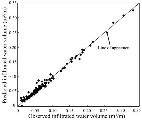
Figure 4.
Comparison between observed and ANN-predicted values for the training dataset.
Table 6.
Statistical performance metrics comparing the ANN model and the TPM.
The network generalization property was tested with the testing and validation sets by applying weights and biases from the training process. The chosen sets displayed the trained network’s competence. The values from testing and validation datasets, were used to predict observed data presented in Figure 5 and Figure 6. The data sets used for testing and validation purposes remained outside the training process since they originated randomly from the data collected. The data possessed their highest concentration and best uniformity surrounding the 1:1 line in both Figure 5 and Figure 6. The observed results matched closely with the results from the ANN model analysis.
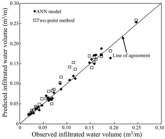
Figure 5.
Comparative analysis of the testing dataset’s observed and predicted values for the ANN model and the TPM.
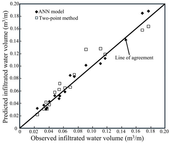
Figure 6.
Comparative analysis of the validation dataset’s observed and predicted values for the ANN model and the TPM.
Table 6 contains statistical parameters that evaluate the ANN model assessment during its testing and validation stages. The predicted values for showed strong agreement with observed results according to the data presented in Table 6 for both datasets. The testing set achieved optimized results because its RMSE reached 0.008 m3/m and CRM reached 0.9%, making both parameters close to zero. The evaluation results indicated close relationships between parameters since R2 held a value of 98.1%, while E reached 98.2%, and OI measured 97.2%. The minimum RMSE value (0.978 m3/m) and CRM value (3.4%) reached nearly zero for the validation process. The statistical values R2 (97.8%), E (96.7%), and OI (95.7%) approximated the value of one. The excellent concurrence between experimental and ANN-predicted results becomes evident through these findings. The ANN model demonstrated strong predictive power when determining accurate values for infiltrated water volume .
3.5. Comparative Analysis of the TPM and the ANN Model
The effectiveness of the selected ANN model was assessed by comparing its performance against the TPM, which served as a benchmark for evaluation. Figure 5 and Figure 6 illustrate that, while TPM produced some significantly inaccurate predictions, the majority of its forecasts were within an acceptable range. In contrast, the ANN model consistently demonstrated superior predictive accuracy when tested using both training and validation datasets. The inconsistencies observed in TPM underscore their inherent unreliability, reinforcing its inadequacy as a robust forecasting technique. Meanwhile, the ANN model exhibited strong agreement with experimental data across all phases—training; testing; and validation—as evidenced by the results in Figure 4, Figure 5 and Figure 6.
A detailed statistical evaluation was conducted to compare the performance of the ANN model and the TPM, as summarized in Table 6. The results indicated that the ANN model outperformed the TPM across key statistical metrics. The R2 derived from the ANN testing dataset was only 2.55% lower than that obtained from the TPM, demonstrating comparable predictive accuracy. However, the RMSE of the TPM (0.014 m3/m) was nearly twice that of the ANN model, signifying a greater margin of error in the former. Furthermore, the efficiency coefficient (E) of the ANN model was 4.03% higher, reflecting improved predictive capability. Similarly, the OI for the ANN model was closer to unity than that of the TPM, reinforcing its superior fit to the experimental data. Additionally, the CRM for the TPM was approximately nine times greater than that of the ANN testing set, highlighting the ANN model’s reduced residual error and enhanced accuracy in predicting infiltrated water volume .
A comparative analysis conducted using the ANN validation dataset (Table 6) further substantiated these findings. The TPM exhibited an R2 accuracy that was 4.7% lower than that of the ANN model during testing. Additionally, the RMSE for the TPM (0.013 m3/m) was nearly twice that of the ANN model, while the ANN model demonstrated a 4.7% higher E value. Moreover, the ANN model’s OI values in the testing phase were notably closer to unity than those obtained through TPM, confirming its superior predictive performance. Lastly, the CRM for the TPM was approximately 1.5 times greater than that of the ANN model in the testing phase, further underscoring the ANN model’s enhanced reliability and precision in forecasting infiltrated water volume.
The relative errors of computed values appear in Figure 7 and Figure 8, which evaluate data from testing and validation using the volume balance model and ANN model. The data presented in these figures indicated that the outcome models exhibited diverse results. Each point in TPM calculations marked an average relative error of 15.5% when testing data were used or an average relative error of 13.6% while working with validation data. Basing the method on two-point data produced equivalent average relative errors for validation and testing results. ANN established corresponding results of 7.4% and 11.3% for both data sets. A decrease in the reduction capacity of the TPM occurred due to these factors. Furthermore, the TPM tended to produce significant overpredictions and underpredictions in estimating furrow infiltration, whereas the ANN model exhibited only minor deviations. Overall, although the TPM provided acceptable predictions of the infiltrated volume, its accuracy was consistently lower than that of the ANN model.
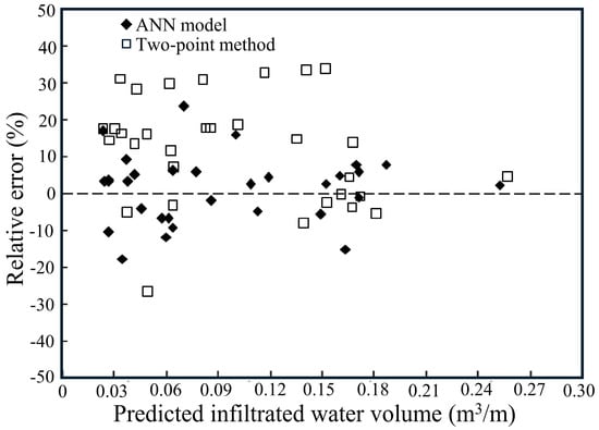
Figure 7.
Analysis of the ANN model’s and the TPMs relative errors for the test dataset.
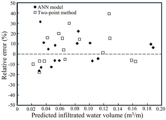
Figure 8.
Analysis of the ANN model’s and the TPMs relative errors for the validation dataset.
The determination of soil infiltration volume using the ANN model relies on a concise set of four parameters, offering a streamlined approach to this complex calculation. In contrast, the traditional TPM necessitates a considerably larger array of parameters, the collection and processing of which demand a substantial investment of time and resources. Employing the ANN model, researchers can significantly reduce the labor and effort required for gathering field data, thereby enhancing efficiency without compromising accuracy. This reduction in fieldwork burden underscores the practical advantages of adopting the ANN model for soil infiltration studies. Sufficient evidence indicates that prediction methods based on ANN and two-point models generate accurate computational results. The prediction produced through ANN outperformed the prediction achieved by the TPM. The ANN application enabled more straightforward input data processing while decreasing the required data set number. The simulation procedure takes less time and provides results with accurate precision.
3.6. GEP Model Performance Analysis
The study found the best GEP algorithm for formulizing with furrow irrigation as presented in (Equation (16))
“The variables in the given equation are expressed in the following units: “” is measured in (L/s), “” is represented in (m), “” is quantified in (min), “” is also recorded in (min), and “” is specified in (cm2)”.
The present study divided the acquired experimental data into three sets for training, validation, and testing purposes. Furthermore, it divided the data into three subsets to evaluate model generalization in the GEP-based approach. The experimental results and predictions from the GEP training and testing phases can be seen in Figure 9 and Figure 10. According to Figure 9 and Figure 10, the experimental measurements matched closely with the results generated through the training and testing processes.
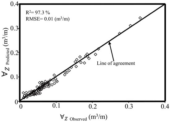
Figure 9.
Comparison between the training dataset’s observed and GEP-predicted values.
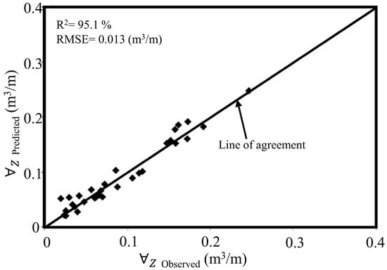
Figure 10.
Comparison between the testing dataset’s observed and GEP-predicted values.
The GEP model exhibited robust generalization capabilities in capturing input-output relationships, as evidenced by its training and testing performance metrics outlined in Table 7. During the training phase, the model demonstrated exceptional predictive accuracy, achieving an R2 of 97.2%, an OI of 97%, an RMSE of 0.01 m3/m, and an MAE of 0.008 m3/m. These metrics underscore the model’s strong alignment with empirical data and its capacity to minimize deviations between predicted and observed values. Notably, the testing phase replicated the model’s reliability, yielding comparable results with an R2 of 95.8%, an OI of 94.5%, an RMSE of 0.01 m3/m, and an MAE of 0.011 m3/m. The marginal reduction in performance metrics during testing—less than 2% for R2 and 2.5% for OI—highlights the model’s consistency and resistance to overfitting. Such minimal variance between the training and testing phases further validates the GEP model’s robustness in extrapolating patterns beyond the training dataset. The close agreement between predicted infiltrated water volumes and experimental measurements (evidenced by near-unity OI values and low RMSE/MAE magnitudes) confirms the model’s efficacy in simulating furrow irrigation dynamics. These results position the GEP framework as a highly reliable tool for forecasting water infiltration under diverse field conditions, offering practical utility in optimizing irrigation management and water resource allocation.
Table 7.
Statistical performance metrics comparing the GEP model and the TPM.
3.7. Comparison Between GEP Model and TPM
Table 7 and Figure 11 offer a comprehensive comparison of the validation outcomes between the GEP model and the TPM. This comparative analysis provides a clear understanding of the relative performance of each approach in predicting the volume of infiltrated water, thereby shedding light on their respective accuracies and overall applicability. Both the table and the figure highlight that the GEP model outperforms the TPM in terms of prediction accuracy. A statistical analysis of the data further confirms a strong correlation between the observed and simulated values, with the GEP model achieving an impressive coefficient of determination (R2) of 96%. In contrast, TPM displayed an R2 value approximately 3.2% lower than that of the GEP model.
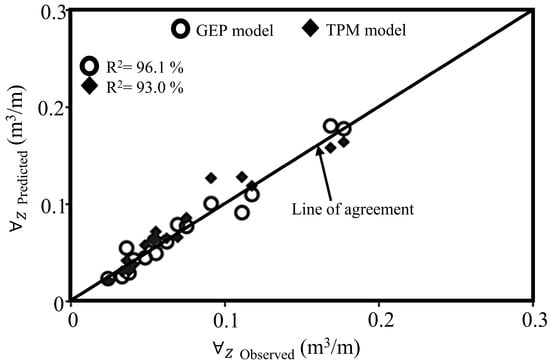
Figure 11.
Comparative analysis of the GEP model’s and the TPMs predicted and observed values using the validation dataset.
The investigation also revealed that the GEP model produced highly satisfactory results, yielding a performance index of 95%, while the TPM resulted in a slightly lower observed index of 92%. The RMSE for the TPM was found to be 0.013 m3/m, which is 1.4 times higher than the RMSE of the GEP model, which was 0.0092 m3/m. Furthermore, the measured average error for the TPM was 0.0094 m3/m, representing a margin 1.3 times greater than the GEP model’s error value of 0.0072 m3/m. Overall, the findings from this investigation suggest that the GEP model can serve as an optimal alternative to the TPM, offering improved accuracy and reliability in water infiltration estimation practices.
Shiri, Kişi [] support this finding by stating that GEP models surpass adaptive neuro-fuzzy inference system (ANFIS) approaches because they directly identify the linkages between dependent and independent variables. GEP models serve computational purposes efficiently and possess user-friendly characteristics that allow non-specialists to use them. According to the authors’ research, the models described by Landeras, López [] require only standard spreadsheet software and personal computers or handheld calculators to run effectively.
3.8. Comparison Between ANN and GEP Model
Table 8 presents a comparative evaluation of ANN and GEP models in predicting under-furrow irrigation systems. The assessment framework utilized three critical statistical metrics—RMSE; OI; and R2—to quantify predictive accuracy across training; testing; and validation datasets. The ANN model demonstrated superior performance in all predictive phases, achieving R2 values of 98.5% during training and maintaining high consistency with values of 98.1% in both the testing and validation phases. In contrast, the GEP model yielded slightly lower yet robust R2 metrics, registering 97.2% (training), 95.7% (testing), and 96.1% (validation). Notably, the ANN framework exhibited an enhanced capacity to interpret the influence of input variables on outcome variables, outperforming the GEP model across all evaluation stages. Both models exhibited strong predictive reliability, as evidenced by RMSE and OI metrics. The ANNs lower RMSE values and OI scores closer to unity underscored its precision in minimizing prediction errors. While the GEP model showed marginally higher error margins, its performance remained commendable, with all R2 values exceeding 95%. These results collectively affirm the utility of both methodologies in simulating infiltration dynamics, with ANN holding a slight edge in accuracy and consistency. The high R2 values (above 95% for both models) and minimal discrepancies between training and validation phases further validate their generalizability, suggesting their applicability in optimizing irrigation strategies under heterogeneous field conditions.
Table 8.
Performance comparison of ANN and GEP models.
During all phases, the ANN model delivers lower RMSE values than the GEP model, as indicated by a 0.005 training value, a 0.008 testing value, and a 0.008 (m3/m) validation value. The RMSE scores from the GEP model reach 0.010 in training, 0.013 in testing, and 0.009 (m3/m) in validation. The testing phase demonstrates that the ANN model prediction accuracy exceeds GEP model accuracy because it produces a lower RMSE of 0.008 than 0.013 (m3/m) from GEP. All phases of ANN model evaluation demonstrate superior outcome results, including 98.5% training, 97.2% testing, and 95.7% validation OI value scores. Predictions from GEP are close to ANN because OI measurements show 97.0% training and 94.4% testing with 94.9% validation performance. The ANN approach demonstrates better data fit than the GEP model during every assessment phase.
The predictive power of the ANN model surpasses GEP model assessments because it produces superior OI scores during all phases, in addition to higher R2 values and lower RMSE scores. The GEP model remains an acceptable substitution for the ANN model because it maintains strong predictive capability, particularly regarding interpretability and computational simplicity, which are important requirements. The ANN framework sustains accurate output during testing, while the GEP framework displays more significant RMSE numbers and reduced OI scores. Both models demonstrate reliable generalization for unseen data according to validation results, but ANN shows a minor advantage in resisting unpredictable data effects. As proven by all statistical criteria, predictions of infiltrated water volume under furrow irrigation demonstrate better performance with ANN models than with GEP models. The GEP model is a viable candidate because it explicitly defines variable relationships, providing benefits regarding computational efficiency and interpretation abilities. Figure 12 depicts the statistical parameters of the employed models.
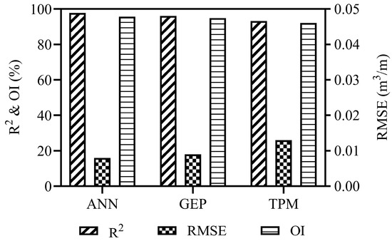
Figure 12.
Statistical performance parameters of the validation dataset for studied models.
3.9. Contribution Analysis for ANN and GEP Models
Sensitivity analysis is designed to examine how a model’s outputs are connected to and affected by its inputs and/or governing factors []. In this study, five input parameters—namely —are likely to influence the output (). To tackle the issue of uncertainty, the ANN model can assess insignificant variables by computing the contribution ratio, which facilitates the inclusion of meaningful variables in the input layer, resulting in the most precise predicted outcomes. The results indicated that the sensitivity analysis has been eliminated from the predictive model due to its minimal contribution. In contrast, the average contributions of to were found to be 19.96%, 30.04%, 26.19%, and 24.81%, respectively, as illustrated in Figure 13a.
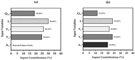
Figure 13.
Contribution analysis of input variables for (a) ANN and (b) GEP models.
Additionally, for GEP, a sensitivity analysis was performed to evaluate the impact of closely related predictor variables () on under-furrow irrigation. A frequency value ranging from zero to one was calculated, where a value nearing 1.0 indicates that this variable has been present in 100% of the top thirty programs generated by GEP. This methodology is commonly employed in GP-based analyses []. The frequency values for the predictor variables are depicted in Figure 13b. As shown, and are more sensitive (23.83% and 23.64%, respectively) to , followed by (21.08%) and (19.91%). Furthermore, demonstrated a lower accuracy (11.51%) compared to the other infiltration parameters.
3.10. Practical Implications for Field Practitioners
Usually, ANN and GEP artificial intelligence (AI) models estimate infiltration water volume better than conventional prediction techniques like TPM. Learning small data patterns and interactions was simplified by their ability to record complex, nonlinear correlations among variables. Such capabilities are especially beneficial when dealing with heterogeneous soil properties and fluctuating environmental conditions, where conventional assumptions may fall short. Based on water advance phase concepts, TPM is achieved with basic volume balance. This approach ignores the complex dynamics in systems with significant nonlinearity or unpredictability, even if computationally efficient and easy to use. Still, the TPM comes in really handy in several contexts: (1) Limited Data Environments: When available data are scarce or exhibits low variability, the TPM can serve as an effective preliminary assessment tool. (2) Routine Applications: For scenarios requiring quick, approximate estimates without the need for complex modeling, the TPM provides a practical solution. and (3) Baseline Comparisons: The TPM can also function as a reference standard to benchmark the performance of more advanced AI models as it considers the whole infiltration parameters “”. AI models can achieve better accuracy by understanding complicated relationships, but in situations where simplicity, quick evaluations, or limited computing power and large data gathering are needed, the TPM remains essential.
The “black-box” nature of the ANN model allows it to understand complex, nonlinear relationships in the data, leading to better prediction accuracy, which is crucial when accuracy matters a lot. For instance, in the current study, the ANN model required fewer variables by eliminating the variable, which had a weak impact on the outcome. By means of improved interpretability, the GEP model helps practitioners to build unambiguous mathematical links between input and output variables. Especially in field applications where the justification for predictions has equal relevance to the predictions themselves, this clarity improves understanding of the fundamental processes and helps in informed decision-making, although it requires the same number of variables as TMP. This work compares the accuracy of the models, considering their various advantages and constraints. Focusing on either precision or interpretability, this viewpoint seeks to help practitioners choose the most appropriate approach depending on the criteria of their field applications.
4. Conclusions
Infiltration dynamics constitute a critical parameter in agricultural water management, serving as a cornerstone for the design and optimization of irrigation systems. Accurate quantification of infiltrated water volume is essential to ensure resource efficiency and crop productivity, necessitating advanced computational methodologies. It is complex to estimate infiltrated water volumes . For furrow irrigation, any experimental analysis where many equations under different soils and environmental conditions are required. Consequently, it will be difficult to express them with a universal equation. The two-point method (TPM) could potentially address this issue, but it requires numerous variables. This study explores the use of machine learning (ML) techniques to overcome these limitations. In this context, ANNs emerge as a robust analytical tool, capable of delivering precise predictions through adaptive learning mechanisms. The present study employed a feedforward MLP-ANN architecture, leveraging a backpropagation algorithm to iteratively refine synaptic weights and minimize prediction errors. The network was structured in a 4-5-1 configuration, comprising four input neurons (representing hydraulic and geometric variables), five hidden neurons for nonlinear transformation, and a single output neuron. Input parameters included inflow rate : governing water delivery dynamics. furrow length : defining the spatial scale of irrigation. waterfront advance time at Furrow Terminus : characterizing temporal progression. infiltration opportunity time : reflecting cumulative exposure duration. The output variable , was modeled independently to isolate its relationship with the aforementioned inputs, with negligible influence from the inflow cross-sectional area .
Additionally, another soft computing technique, gene expression programming (GEP), was employed to estimate directly based on the same five input variables. The GEP model was trained using 70% of the available data, tested on the remaining 20%, and validated with the last 10%. The model’s performance was evaluated by comparing the predictions from GEP and TPM with experimental results. The comparisons revealed reasonable agreement between the predicted and observed data for TPM but stronger alignment for the GEP model. The best R2 and OI values achieved were 96% and 95%, respectively, while the minimum RMSE and MAE values recorded were 0.0092 and 0.0072 m3/m, respectively, during the validation phase of GEP. These findings demonstrate that the GEP model can effectively predict in-furrow irrigation systems. Finally, the study compared the ANN and GEP models for predicting in-furrow irrigation setups. The evaluation framework utilized three key statistical metrics—RMSE; OI; and R2—to measure predictive accuracy across training; testing; and validation datasets. All statistical indicators showed superior performance in predicting with ANN models compared to GEP models. However, the GEP model remains a strong contender as it clearly defines relationships among variables, offering advantages in computational efficiency and interpretability. To ensure generalizability, both models were rigorously validated across a range of furrow irrigation scenarios, incorporating various soil textures and hydraulic conditions. This systematic calibration allowed the network to accurately capture complex, nonlinear interactions between input factors and infiltration results, aligning closely with empirical data. Furthermore, the sensitivity analysis investigated non-important variables by calculating the contribution ratio, which allows the introduction of valuable variables to the input layer and gives the most accurately predicted output results.
Author Contributions
Conceptualization, F.R.; Data curation, A.A.A. and F.R.; Formal analysis, A.A.A. and F.R.; Methodology, A.A.A. and F.R.; Project administration, A.A.A.; Software, A.A.A. and F.R.; Validation, A.A.A. and F.R.; Writing—original draft, A.A.A. and F.R.; Writing—review and editing, A.A.A., M.A.M., A.E.-S., F.R., M.E. and N.A. All authors have read and agreed to the published version of the manuscript.
Funding
This project was funded by the National Plan for Science, Technology and Innovation (MAARIFAH), King Abdulaziz City for Science and Technology, Kingdom of Saudi Arabia, award number (WAT1152) and the APC was funded by (MAARIFAH).
Data Availability Statement
The data can be provided by the appropriate author upon a reasonable request.
Acknowledgments
This project was funded by the National Plan for Science, Technology and Innovation (MAARIFAH), King Abdulaziz City for Science and Technology, Kingdom of Saudi Arabia, Award Number (WAT1152).
Conflicts of Interest
The authors declare no conflict of interest.
References
- Amami, R.; Ibrahimi, K.; Sher, F.; Milham, P.; Ghazouani, H.; Chehaibi, S.; Hussain, Z.; Iqbal, H.M.N. Impacts of Different Tillage Practices on Soil Water Infiltration for Sustainable Agriculture. Sustainability 2021, 13, 3155. [Google Scholar] [CrossRef]
- Liu, Y.; Cui, Z.; Huang, Z.; López-Vicente, M.; Wu, G.-L. Influence of soil moisture and plant roots on the soil infiltration capacity at different stages in arid grasslands of China. CATENA 2019, 182, 104147. [Google Scholar] [CrossRef]
- Chavoshi, A.; Dashtian, H.; Bakhshian, S.; Young, M.H.; Niyogi, D. PINN-SM: A Physics-Informed Neural Networks Model for Vadose Zone Soil Moisture Profile Prediction. Authorea Prepr. 2024. [Google Scholar] [CrossRef]
- Singh, A.; Gaurav, K. PIML-SM: Physics-Informed Machine Learning to Estimate Surface Soil Moisture from Multisensor Satellite Images by Leveraging Swarm Intelligence. IEEE Trans. Geosci. Remote Sens. 2024, 62, 4416913. [Google Scholar] [CrossRef]
- Bautista, E.; Schlegel, J.L. Estimation of Infiltration and Hydraulic Resistance in Furrow Irrigation, with Infiltration Dependent on Flow Depth. Trans. ASABE 2017, 60, 1873–1884. [Google Scholar] [CrossRef]
- Salahou, M.K.; Jiao, X.; Lü, H.; Guo, W. An improved approach to estimating the infiltration characteristics in surface irrigation systems. PLoS ONE 2020, 15, e0234480. [Google Scholar] [CrossRef]
- Al-Janabi, A.M.S.; Ghazali, A.H.; Yusuf, B. Modified models for better prediction of infiltration rates in trapezoidal permeable stormwater channels. Hydrol. Sci. J. 2019, 64, 1918–1931. [Google Scholar] [CrossRef]
- Javadi, A.; Ostad-Ali-Askari, K. Effect of Different Irrigation Managements on Infiltration Equations and Their Coefficients. CivilEng 2023, 4, 949–965. [Google Scholar] [CrossRef]
- Ebrahimian, H.; Liaghat, A. Field evaluation of various mathematical models for furrow and border irrigation systems. Soil Water Res. 2011, 6, 91–101. [Google Scholar] [CrossRef]
- Adamu, T.; Ayana, M.; Aregay, G. Optimization of furrow irrigation decision variables: The case of wonji shoa sugar estate, Ethiopia. Discov. Water 2022, 2, 10. [Google Scholar] [CrossRef]
- Valipour, M. Comparison of Surface Irrigation Simulation Models: Full Hydrodynamic, Zero Inertia, Kinematic Wave. J. Agric. Sci. 2012, 4, p68. [Google Scholar] [CrossRef]
- Elliott, R.L.; Walker, W.R. Field Evaluation of Furrow Infiltration and Advance Functions. Trans. ASAE 1982, 25, 0396–0400. [Google Scholar] [CrossRef]
- Bautista, E.; Clemmens, A.J.; Strelkoff, T.S. Structured Application of the Two-Point Method for the Estimation of Infiltration Parameters in Surface Irrigation. J. Irrig. Drain. Eng. 2009, 135, 566–578. [Google Scholar] [CrossRef]
- Bautista, E.; Strelkoff, T.S.; Clemmens, A.J. Errors in Infiltration Calculations in Volume-BalanceModels. J. Irrig. Drain. Eng. 2012, 138, 727–735. [Google Scholar] [CrossRef]
- Panahi, A.; Seyedzadeh, A.; Maroufpoor, E. Investigating the midpoint of a two-point method for predicting advance and infiltration in surface irrigation. Irrig. Drain. 2021, 70, 1095–1106. [Google Scholar] [CrossRef]
- Kargas, G.; Mindrinos, L. A new method of estimating infiltration parameters for furrow irrigation. Irrig. Drain. 2024, 74, 658–672. [Google Scholar] [CrossRef]
- Maghferati, H.R.; Chari, M.M.; Afrasiab, P.; Delbari, M. Investigation of various volume–balance methods in surface irrigation. Arab. J. Geosci. 2021, 14, 241. [Google Scholar] [CrossRef]
- Panahi, M.; Khosravi, K.; Ahmad, S.; Panahi, S.; Heddam, S.; Melesse, A.M.; Omidvar, E.; Lee, C.-W. Cumulative infiltration and infiltration rate prediction using optimized deep learning algorithms: A study in Western Iran. J. Hydrol. Reg. Stud. 2021, 35, 100825. [Google Scholar] [CrossRef]
- Wang, X. The artificial intelligence-based agricultural field irrigation warning system using GA-BP neural network under smart agriculture. PLoS ONE 2025, 20, e0317277. [Google Scholar] [CrossRef]
- Abdulsalam, J.; Lawal, A.I.; Setsepu, R.L.; Onifade, M.; Bada, S. Application of gene expression programming, artificial neural network and multilinear regression in predicting hydrochar physicochemical properties. Bioresour. Bioprocess. 2020, 7, 62. [Google Scholar] [CrossRef]
- Raza, A.; Vishwakarma, D.K.; Acharki, S.; Al-Ansari, N.; Alshehri, F.; Elbeltagi, A. Use of gene expression programming to predict reference evapotranspiration in different climatic conditions. Appl. Water Sci. 2024, 14, 152. [Google Scholar] [CrossRef]
- Al-Janobi, A.; Aboukarima, A.; Ahmed, K. Modeling water infiltration rate under conventional tillage systems on a clay soil using artificial neural networks. Aust. J. Basic Appl. Sci. 2010, 4, 3869–3879. [Google Scholar]
- El Marazky, M.S.A.; Aboukarima, A.M.; Guirguis, A.E.; Egela, M.I. Water infiltration as affected by tillage methods, plowing depth and wheel traffic. J. Soil Sci. Agric. Eng. 2007, 32, 2019–2033. [Google Scholar] [CrossRef]
- Valiantzas, J.; Aggelides, S.; Sassalou, A. Furrow infiltration estimation from time to a single advance point. Agric. Water Manag. 2001, 52, 17–32. [Google Scholar] [CrossRef]
- Alvarez, J.A.R. Estimation of advance and infiltration equations in furrow irrigation for untested discharges. Agric. Water Manag. 2003, 60, 227–239. [Google Scholar] [CrossRef]
- Holzapfel, E.A.; Jara, J.; Zuniga, C.; Marino, M.A.; Paredes, J.; Billib, M. Infiltration parameters for furrow irrigation. Agric. Water Manag. 2004, 68, 19–32. [Google Scholar] [CrossRef]
- Playán, E.; Rodriguez, J.; Garcia-Navarro, P. Simulation model for level furrows. I: Analysis of field experiments. J. Irrig. Drain. Eng. 2004, 130, 106–112. [Google Scholar] [CrossRef]
- Mateos, L.; Oyonarte, N.A. A spreadsheet model to evaluate sloping furrow irrigation accounting for infiltration variability. Agric. Water Manag. 2005, 76, 62–75. [Google Scholar] [CrossRef]
- Sepaskhah, A.; Shaabani, M. Infiltration and hydraulic behaviour of an anguiform furrow in heavy texture soils of Iran. Biosyst. Eng. 2007, 98, 248–256. [Google Scholar] [CrossRef]
- FAO-UNESCO. Soil Map of the World, Revised Legend. In World Soil Resources Report; FAO-UNESCO: Rome, Italy, 1988; Volume 60. [Google Scholar]
- O’Reilly, G.; Bezuidenhout, C.C.; Bezuidenhout, J.J. Artificial neural networks: Applications in the drinking water sector. Water Sci. Technol. Water Supply 2018, 18, 1869–1887. [Google Scholar] [CrossRef]
- Kumar, A.; Sodhi, S.S. Some Modified Activation Functions of Hyperbolic Tangent (TanH) Activation Function for Artificial Neural Networks. In Proceedings of the International Conference on Innovations in Data Analytics, West Bengal, India, 29–30 November 2022; Springer: Berlin/Heidelberg, Germany, 2022. [Google Scholar]
- Aljarah, I.; Faris, H.; Mirjalili, S. Optimizing connection weights in neural networks using the whale optimization algorithm. Soft Comput. 2018, 22, 1–15. [Google Scholar] [CrossRef]
- Koza, J.R. Genetic programming as a means for programming computers by natural selection. Stat. Comput. 1994, 4, 87–112. [Google Scholar] [CrossRef]
- Ferreira, C. Gene Expression Programming: Mathematical Modeling by an Artificial Intelligence; Springer: Berlin/Heidelberg, Germany, 2006; Volume 21. [Google Scholar]
- Sharma, P. Gene expression programming-based model prediction of performance and emission characteristics of a diesel engine fueled with linseed oil biodiesel/diesel blends: An artificial intelligence approach. Energy Sources Part A Recover. Util. Environ. Eff. 2025, 47, 1385–1399. [Google Scholar] [CrossRef]
- GEPSOFT. GEPSOFT GeneXproTools—Data Modeling and Analysis Software. 2014. Available online: https://www.gepsoft.com/ (accessed on 1 January 2025).
- Seyedzadeh, A.; Panahi, A.; Maroufpoor, E.; Merkley, G.P. Subsurface shape factor for surface irrigation hydraulics. Irrig. Drain. 2022, 71, 687–696. [Google Scholar] [CrossRef]
- Walker, W.R.; Skogerboe, G.V. Surface Irrigation. Theory and Practice; Prentice-Hall: Saddle River, NJ, USA, 1987. [Google Scholar]
- Kiefer, F., Jr. Average Depth of Absorbed Water in Surface Irrigation; Special Publication; Civil Engineering Department, Utah State University: Logan, UT, USA, 1965. [Google Scholar]
- Chicco, D.; Warrens, M.J.; Jurman, G. The coefficient of determination R-squared is more informative than SMAPE, MAE, MAPE, MSE and RMSE in regression analysis evaluation. PeerJ Comput. Sci. 2021, 7, e623. [Google Scholar] [CrossRef]
- Soyer, M.A.; Tüzün, N.; Karakaş, Ö.; Berto, F. An investigation of artificial neural network structure and its effects on the estimation of the low-cycle fatigue parameters of various steels. Fatigue Fract. Eng. Mater. Struct. 2023, 46, 2929–2948. [Google Scholar] [CrossRef]
- Shiri, J.; Kişi, Ö.; Landeras, G.; López, J.J.; Nazemi, A.H.; Stuyt, L.C. Daily reference evapotranspiration modeling by using genetic programming approach in the Basque Country (Northern Spain). J. Hydrol. 2012, 414–415, 302–316. [Google Scholar] [CrossRef]
- Landeras, G.; López, J.J.; Kisi, O.; Shiri, J. Comparison of Gene Expression Programming with neuro-fuzzy and neural network computing techniques in estimating daily incoming solar radiation in the Basque Country (Northern Spain). Energy Convers. Manag. 2012, 62, 1–13. [Google Scholar] [CrossRef]
- Panigrahi, B.; Razavi, S.; Doig, L.E.; Cordell, B.; Gupta, H.V.; Liber, K. On Robustness of the Explanatory Power of Machine Learning Models: Insights from a New Explainable AI Approach Using Sensitivity Analysis. Water Resour. Res. 2025, 61, e2024WR037398. [Google Scholar] [CrossRef]
- Mollahasani, A.; Alavi, A.H.; Gandomi, A.H. Empirical modeling of plate load test moduli of soil via gene expression programming. Comput. Geotechnol. 2011, 38, 281–286. [Google Scholar] [CrossRef]
Disclaimer/Publisher’s Note: The statements, opinions and data contained in all publications are solely those of the individual author(s) and contributor(s) and not of MDPI and/or the editor(s). MDPI and/or the editor(s) disclaim responsibility for any injury to people or property resulting from any ideas, methods, instructions or products referred to in the content. |
© 2025 by the authors. Licensee MDPI, Basel, Switzerland. This article is an open access article distributed under the terms and conditions of the Creative Commons Attribution (CC BY) license (https://creativecommons.org/licenses/by/4.0/).