Next Article in Journal
Water Quality Improvement Performance of Geotextiles Within Permeable Pavement Systems: A Critical Review
Next Article in Special Issue
Factors Affecting Phosphorous in Groundwater in an Alluvial Valley Aquifer: Implications for Best Management Practices
Previous Article in Journal
Dissolved Oxygen Concentration Interlaboratory Comparison: What Can We Learn?
Previous Article in Special Issue
Comparative Assessment of Stormwater and Nonpoint Source Pollution Best Management Practices in Suburban Watershed Management
 
 
Correction published on 18 September 2013, see Water 2013, 5(3), 1440.
Article

Mountain Pine Beetles, Salvage Logging, and Hydrologic Change: Predicting Wet Ground Areas

Ministry of Forests, Lands & Natural Resource Operations, 5th Floor, 1044 5th Avenue Prince George, BC V2L5G4, Canada
*
Author to whom correspondence should be addressed.
Water 2013, 5(2), 443-461; https://doi.org/10.3390/w5020443
Submission received: 28 January 2013 / Revised: 26 March 2013 / Accepted: 2 April 2013 / Published: 15 April 2013
(This article belongs to the Special Issue Ecological Watershed Management)

Abstract

:
The mountain pine beetle epidemic in British Columbia has covered 18.1 million hectares of forest land showing the potential for exceptionally large-scale disturbance to influence watershed hydrology. Pine stands killed by the epidemic can experience reduced levels of evapotranspiration and precipitation interception, which can translate into an increase in soil moisture as observed by some forest practitioners during salvage logging in the epicenter of the outbreak. They reported the replacement of summer ground, dry firm soil areas, with winter ground areas identified by having wetter, less firm soils upon which forestry equipment operation is difficult or impossible before winter freeze-up. To decrease the likelihood of soil disturbance from harvesting, a set of hazard indicators was developed to predict wet ground areas in areas heavily infested by the mountain pine beetle. Hazard indicators were based on available GIS data, aerial photographs, and local knowledge. Indicators were selected by an iterative process that began with office-based selection of potential indicators, model development and prediction, field verification, and model refinement to select those indicators that explained most field data variability. Findings indicate that the most effective indicators were lodgepole pine content, understory, drainage density, soil texture, and the topographic index.

1. Introduction

The mountain pine beetle (MPB) epidemic in British Columbia is the most severe bark beetle infestation recorded in the history of North America. Its origin is the result of climate change, specifically winter minimum temperatures that are too warm to kill beetle larvae in combination with effective forest fire suppression that maintained an abundant mature pine tree population [1,2]. The beetle infestation increased dramatically from 2000 to 2006 progressing from an endemic outbreak to an epidemic that has presently affected an area of some 18.1 million hectares. The scale of this infestation is a significant challenge for forestry and watershed management.
The initial response to the infestation was to increase the allowable cut within the most heavily infested areas where the outbreak began to recover the economic value of attacked pine stands and to expedite the regeneration of new forests in those areas. Salvage logging operations reported difficulties due to a loss in summer ground between 2003 and 2005. That is, during those harvest years forest practitioners encountered wet soils that made equipment operation difficult or impossible where they had expected to encounter dry soils capable of supporting heavy equipment. The frequency of these observations over the landscape signaled a possible change in water balance and subsequent ecology of affected areas.
Mountain pine beetles (Dendroctonous pondorosae, Hopkins) can affect forest hydrology by killing pine tree stands. MPB generally burrow into pine trees in the lower bole where they create galleries to mate and lay their eggs. During this process they pass through the phloem and once eggs hatch in the early summer and fall, larvae feed on the phloem, which increases tree stress and lowers transpiration [3]. When a tree is attacked by a sufficient number of beetles it dies. Once dead, the tree passes from green to red attack where the pine needles first change from green to red the first year post-infestation, after which they progress to grey attack where trees lose their needles and then fine branches over the next couple of years. During this transition, dead and dying pine tree stands will have lower evapotranspiration rates than stands of live trees [4,5,6]. The loss of pine needles and branches decreases precipitation interception, which can vary between 15% and 35% among coniferous forest stands depending upon precipitation amount and form, tree species, and stand characteristics [7,8,9]. Transpiration also decreases or ceases, which will also increase soil moisture. The loss of transpiration can be substantial, for example lodegepole pine stand transpiration accounted for 50% and 61% of total evapotranspiration (ET) in pine stands of southeastern Wyoming [10]. Although the loss in transpiration may account for lower amounts of water removed from the soil, interception is still considered the important factor accounting for “watering-up”, a term used to identify an increase in groundwater table elevation following harvesting [11]. As MPB affected trees progress to grey attack they drop needles decreasing the interception of precipitation up to 50% above pre-infestation levels [12]. This exceeds the reduction of evapotranspiration between six and 39% observed from sub-boreal watersheds subjected to harvesting alone [13]. Increased delivery of precipitation to the ground (i.e., net precipitation) may be stored or moved through the watershed unless remaining live trees or an understory transpire sufficiently as noted by Brown [14]. Where increased net precipitation is stored, water table elevation can increase and soils may “water-up” [15]. If it moves through the watershed and is exported, the annual water yield will increase [16,17].
The project discussed here developed a watershed level hydrologic hazard assessment procedure to assess the relative hazard of experiencing wet soils during salvage logging due to increased water table elevation and/or delayed surface drainage resulting from watershed characteristics and the MPB infestation. Wet ground during salvage operations increases the likelihood of soil disturbance, which can decrease productivity, increase silviculture costs, and increase surface erosion that can lead to water quality problems for streams receiving run-off. Field observations were used to assess effectiveness of the hazard assessment process as well as to provide insight on the cumulative effect of the MPB infestation and salvage logging on soil hydrology. This project is also distinctive because it examines logging operations under a set of ecological conditions related to massive insect outbreak whereas works most often cited in the literature are the effects of salvage operations following wildfire [18].

2. Materials and Methods

2.1. Study Area and Climate Analysis

The study focused on watersheds in the Vanderhoof Forest District of British Columbia (Figure 1). The epidemic began in this forest district and it was particularly affected by the outbreak because forests of the area are more than 80% composed of lodgepole pine (Pinus contorta var. latifolia).
Figure 1. Location of the Vanderhoof Forest District in British Columbia Canada.
Water 05 00443 g001
To predict the hazard of wet ground within third and fourth order watersheds, each watershed in the district was systematically evaluated using the same indicators to assess how likely it would be to have wet ground relative to other watersheds. Due to the absence of hydrologic information at the scale of our investigation, two hazard assessment approaches were taken. The a priori approach predicted watershed hazard based upon indicators selected from the hydrologic literature as well as professional opinion. The post-hoc approach consisted of an exploratory statistical review of field data to identify indicators most effective at explaining field data variability. In addition to hazard analysis a climate analysis was completed to identify change in precipitation timing and quantity.
To assess climatic trend influence on field observations a review of climate information and an assessment of climatic trends were conducted based on five different Meteorological Services Canada (MSC) weather stations near Vanderhoof. This analysis focuses on data collected between 1980 and 2007 because the weather stations were most similar, being at the same elevation and only 2.2 km apart. Further, this recent period of data provides a relevant climatic context to concerns about the loss of summer ground. Annual and seasonal trend analysis for precipitation was assessed using a t-test of slope.

2.2. The a Priori Approach

The a priori approach used two categories of hazard indicators, specifically those that infer the potential for increased net precipitation and those that infer the potential for retention of increased net precipitation in the soil (Table 1).
Table 1. Hazard indicators used to assess likelihood of wet ground areas in the Vanderhoof Forest District through the a priori approach.
Factors enhancing net precipitation (mountain pine beetle (MPB) and Forest Stand Conditions)
Mature Pine CoverAs the proportion of mature pine (>60 years old) infected by MPB increases, transpiration decreases at the watershed level.
Grey Attack As the infested tree progresses from red to grey attack its interception role decreases. Also, older attack areas have experienced increased net precipitation for a longer time period.
MPB SeverityAerial surveys completed in 2004 were classified as light (1%–10%), moderate (11%–29%), or severe infestation (>30%).
Potential for Increased Retention of Soil Water
Soil Moisture Soil moisture categories based on biogeoclimatic zone classifications grouped as well drained (very xeric–mesic soils), imperfectly drained (sub-hygric soils), and poorly drained (Hygric–Hydric soils).
Watershed % with Sensitive SoilsSoil and landform maps of the Vanderhoof Forest District (1:50,000) were coded to identify fine texture soil types (ex. lacustrine) prone to shallow or perched water tables along with organic soils. Fine surface and organic soils will likely have higher ambient soil moisture conditions and will respond more to increased net precipitation than coarser well-drained soil types.
Understory ScoreMulti-storied stands may not see an increase in net precipitation after MPB infestation [14,19]. Understory regeneration increases in the sequence of sub-boreal spruce dry cold, dry warm, and moist cool, as well as Engelmann Spruce Subalpine Fir zone to more than 1000 stems/ha [20], which reduces net precipitation.
Drainage DensityProvides an estimate of how efficiently water leaves an area during storms [21] by providing an index of relative distance between where rain falls and flowing channels [22].
Net precipitation indicators targeted forest condition and beetle infestation characteristics such as available rearing habitat (mature pine content), amount of grey attack stage pine trees and the infestation severity data from the 2004 aerial overview survey. Retention indicators focused on watershed characteristics influencing snowmelt and runoff conditions such as understory condition, drainage density, as well as soil texture and moisture. Aspect was excluded because the topography of the area was relatively flat and did not allow adequate watershed differentiation.
The a priori hazard score was calculated as [Equation (1)]:
Hazard = potential for increased net precipitation × potential for retention of increased net precipitation
Scores were normalized to a scale of 100 and hazard categories were assessed as low for the first quartile (0–25), moderate for the second quartile (25–50), and high for the third and fourth quartile (50–100).

2.3. The Post-Hoc Approach

Hazard indicators were identified in the post-hoc approach using a coarse and fine filtering approach [23]. The coarse filtering approach consisted of a principle components analysis (PCA) of field data from seven of the 17 sites to identify groups of correlated hazard indicators that explained a high proportion of data variability [24]. Hazard indicators include those identified for the a priori approach as well as the topographic index [25,26] and relief ratio [24]. Once groups of indicators were identified, they were fine filtered using a stepwise general linear model, which identified those indicators that had the highest predictive power for identifying field verified “wet sites”. Pos-hoc model verification was completed by comparing predicted and observed conditions at the ten sites not used for model-building

2.4. Site Classification and Study Design

A total of 17 watersheds were chosen for study in 2005–2007 using the first hazard assessment results. These include six low hazard, four moderate hazard, and seven high hazard watersheds as identified by the a priori method (Table 2).
The prominence of high and low hazard watersheds was intentional to maximize the amount of data gathered to identify field differences between these classifications. Study sites were in pine dominated stands with dry to average soil moisture conditions and they were located along hill slopes in lower watershed reaches to ensure similar sampling environments between watersheds. Within these 17 watersheds, seven detailed assessment study areas were established in 2005 while the remaining ten qualitative assessment areas were chosen in 2005 and 2006 (Table 2). Field information from 2006 and 2007 was used for the a priori and post-hoc assessment approach because those sampling seasons provided the most consistent datasets across all the detailed and qualitative assessment sites.
Table 2. The a priori predicted hydrologic hazard for studied watersheds, their harvest level and the assessment approach used in 2006–2007.
Watershed Assessment Approach Harvest Level (% of basin) Hydrologic Hazard—2006
Peta CreekDetailedNo HarvestLow
Angly LakeDetailedNo HarvestLow
Cobb LakeDetailed>30% HarvestLow
Pitka CreekDetailed>30% HarvestLow
ShaydeeQualitative>30% HarvestLow
10330Qualitative<30% HarvestLow
10411Qualitative<30% HarvestModerate
10610Qualitative<30% HarvestModerate
10573Qualitative>30% HarvestModerate
10557Qualitative<30% HarvestHigh
Crystal LakeDetailedNo HarvestHigh
Chowsunkut LakeQualitative>30% HarvestHigh
Targe CreekDetailed>30% HarvestModerate
Belisle CreekDetailed>30% HarvestHigh
Targe Creek-44Qualitative<30% HarvestModerate
10426Qualitative<30% HarvestHigh
10485Qualitative>30% HarvestHigh

2.4.1. Qualitative Assessment Approach

Volumetric soil moisture content (θ) was measured in each watershed at a grey attack stand as well as a bordering harvested area along the same slope at the toe, mid-slope and summit positions at 10, 20, 40, and 60 cm depth. Average soil moisture from the four depths was measured in the late summer and fall, when summer ground issues should be observed, using a Thetaprobe connected to a hand-held reader (Delta-T Devices Ltd., Cambridge, UK). Soil-specific calibration of the Thetaprobe followed the general procedure for calibrating capacitance sensors and provided accuracy of ±1%–3% for our soils [27,28]. Volumetric soil moisture content above 30% was considered to be at levels where harvesting equipment may cause soil disturbance and concurrently experience operational difficulties.

2.4.2. Detailed Assessment Approach

Detailed assessment sites have nine wells located along MPB killed forested pine-leading stands and harvested slopes (Figure 2). Specifically, there are three wells installed along a transect at the level summit, middle slope and toe slope of the harvested and forested sites to study the range of variability in soil hydrologic properties [9,29]. Soil structural-textural conditions were confirmed in proximal pedons to ensure within-site characteristics are as uniform as possible.
Field measurements were gathered at two to three week intervals in spring and summer as well as early fall. These periods were chosen to examine seasonal water table fluctuations. This sampling frequency also allowed for observation of surface ponding, soil saturation, and surface flow due to precipitation as measured by a proximal rain gauge.
Figure 2. Orthophoto image of the Belisle Creek detailed assessment site showing site design (Inset shows Thetaprobes at 10, 20, 40, and 60 cm depth).
Water 05 00443 g002
Shallow wells (<1 m) were excavated by auger and lined with a 4 cm interior diameter PVC pipe [30]. Water table depths were measured at each site using a dipper or electrical buzzer probe [31]. Water table depths less than 60 cm below surface were considered “shallow” and to be an operational concern because the capillary fringe may be as high as 30 cm above the water table indicating a reduced amount of soil available for storage during rainfall events. The amplitude of the capillary fringe was determined by steel rods driven vertically in mineral soil [32] weekly over four growing seasons under similar soil conditions in another as yet unreported study.
To examine potential changes as to how water moves under saturated conditions, field saturated hydraulic conductivity (Kfs) was measured in five watersheds using a simplified falling-head technique [33]. A value of α*-parameter = 12 m−1 was used to calculate Kfs [34]. The five watersheds chosen cover the range of hydrological risks i.e. low, moderate, and high hazard systems as determined by the a priori approach. Kfs data was measured in both forested areas and harvested areas at the summit position to assess harvesting effect (i.e., soil disturbance) on soil drainage. Six randomly chosen 24 m2 grid sampling areas were located within each of the forested and harvested areas. Within each grid, samples were drawn from 12 points.
As soil texture influences hydraulic conductivities, surface soil particle size of the fine soil fraction (<2 mm) was measured at each Kfs sampling point (Table 3) using the hydrometer method [35]. Soils were predominantly coarse and relatively uniform in texture within the top layer (0–10 cm depth) across the sites except at Belisle Creek, which had high clay content (Table 3). Within the sites, forested and clear-cut areas had similar particle size distribution.
Bulk density (Db) information was also gathered to provide an index of soil compaction [36]. Db was calculated on wet volume basis and determined by the core technique [37]), two cores (4 cm long × 5 cm diameter) collected at the mid-point of the 10 and 20 cm depths.
Table 3. Particle-size distribution in top 10 cm soil in the MPB and clearcut for the five selected sites (n = 4).
Site Condition Texture Class Clay (%) (<2 μm) Silt (%) (2–50 μm) Sand (%) (>50 μm)
Belisle CreekForestedSilty clay loam33589
ClearcutSilty clay loam306010
Targe CreekForestedSandy loam103456
ClearcutSandy loam94051
10411ForestedSandy loam83755
ClearcutSandy loam82864
Cobb LakeForestedSandy loam72568
ClearcutSandy loam62866
Pitka CreekForestedSandy loam73657
ClearcutSandy loam63460

2.5. Statistical Analysis

Water table data collected from well sites were log-normally distributed and were transformed prior to Analysis of Variance (ANOVA) and used to identify differences in water table depth across slope location, hazard class, treatment (MPB and cutblock), season, and year using SYSTAT 11® software. Soil moisture measurements were subjected to similar analyses but did not require transformation. ANOVA for soil moisture data was completed using average soil moisture collected from the 10, 20, 40, and 60 cm depths. Significance for all tests was determined at a level of 0.05.
The Kfs values were also log-normally distributed and were transformed accordingly prior to a group t test (PROC TTEST) to compare transformed Kfs and normally distributed soil bulk density data (Db) within sites (MPB vs. clear-cut). All analyses were based on a significance level of p = 0.05.

3. Results and Discussion

3.1. Climate

Analysis identified that annual precipitation has increased over historical levels but not significantly (Table 4). The summers of 2005 and 2007 were the wettest on record. The ratio of summer to winter precipitation has increased significantly since 1997 (Table 4).
Table 4. Precipitation trends between 1980 and 2007 at the Vanderhoof climate station.
Vanderhoof 1980–2007 Trend Change (%) t-Test of slope, differs from 0, 90%
Annual Total PrecipitationIncreasing10.2Not Significant
Winter PrecipitationDecreasing−45.1Significant
Spring PrecipitationIncreasing26.1Not Significant
Summer PrecipitationIncreasing47.0Significant
Fall PrecipitationIncreasing26.4Not Significant
Annual Rain to Snow RatioIncreasing67.0Significant
Annual RainIncreasing33.8Significant
Summer RainIncreasing47.3Significant
Fall RainIncreasing43.9Significant
Between 2001 and 2003, summer precipitation totals (June–September) were within 4% of the 1971–2000 normal of 191 mm. Summer precipitation levels for 2004 and 2005, and 2007 were considerably greater, ranging from 250 to 329 mm or 30%–75% higher than the 30-year normal. Given that summer months are generally wetter now than they were in the earlier period of the climatic record, there may be an effect on trafficability during harvesting activities in areas prone to poor drainage.

3.2. Field Findings

There was a significant slope location and seasonal effect (F2,189 = 55.9, p < 0.001 and F2,189 = 5.9, 
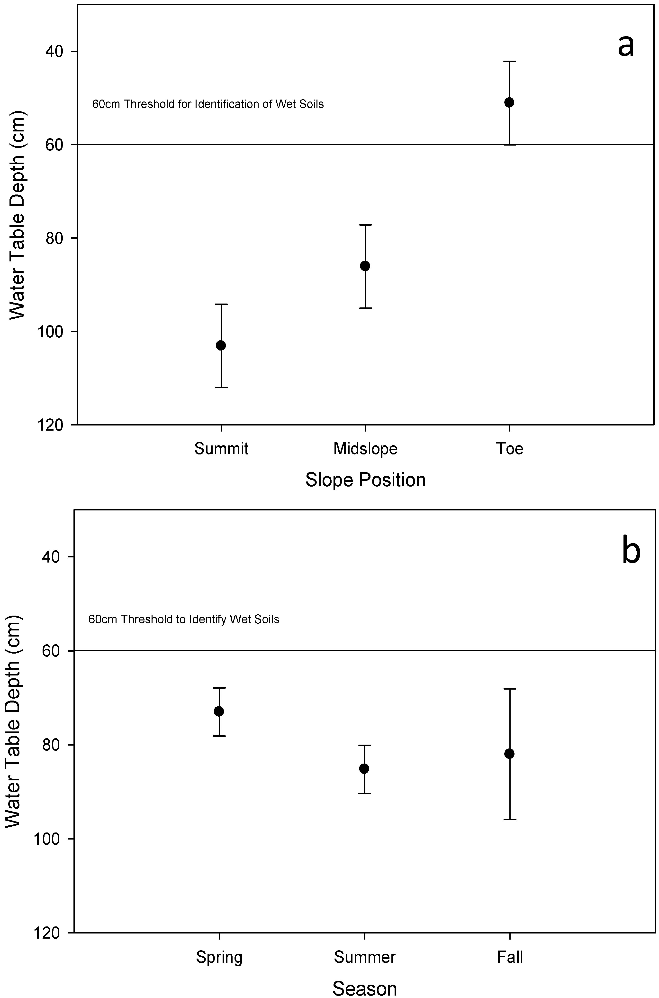
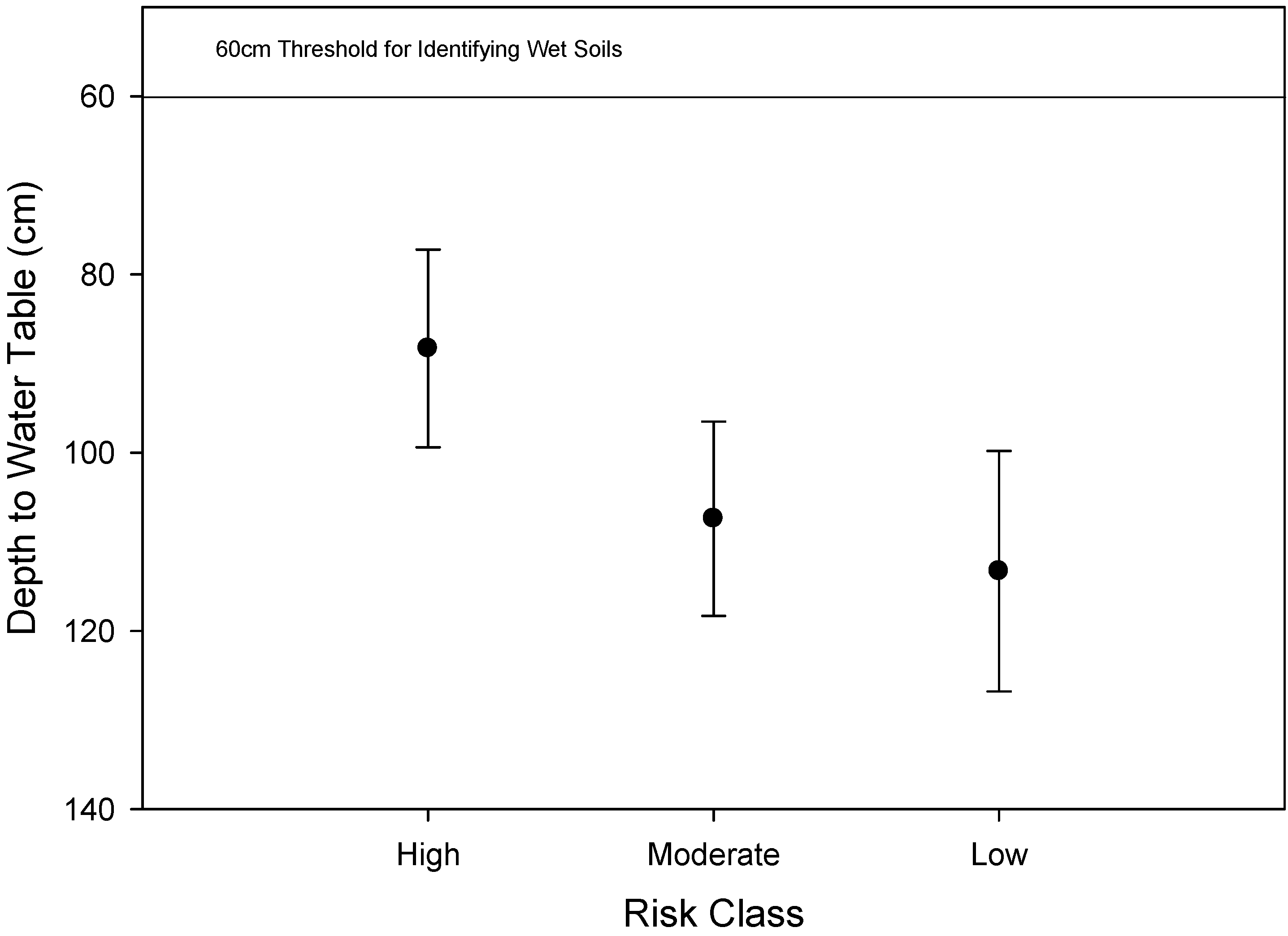
p = 0.003 respectively) on depth to water table across all sites. Toe slope locations had shallower water table levels than the other slope positions (
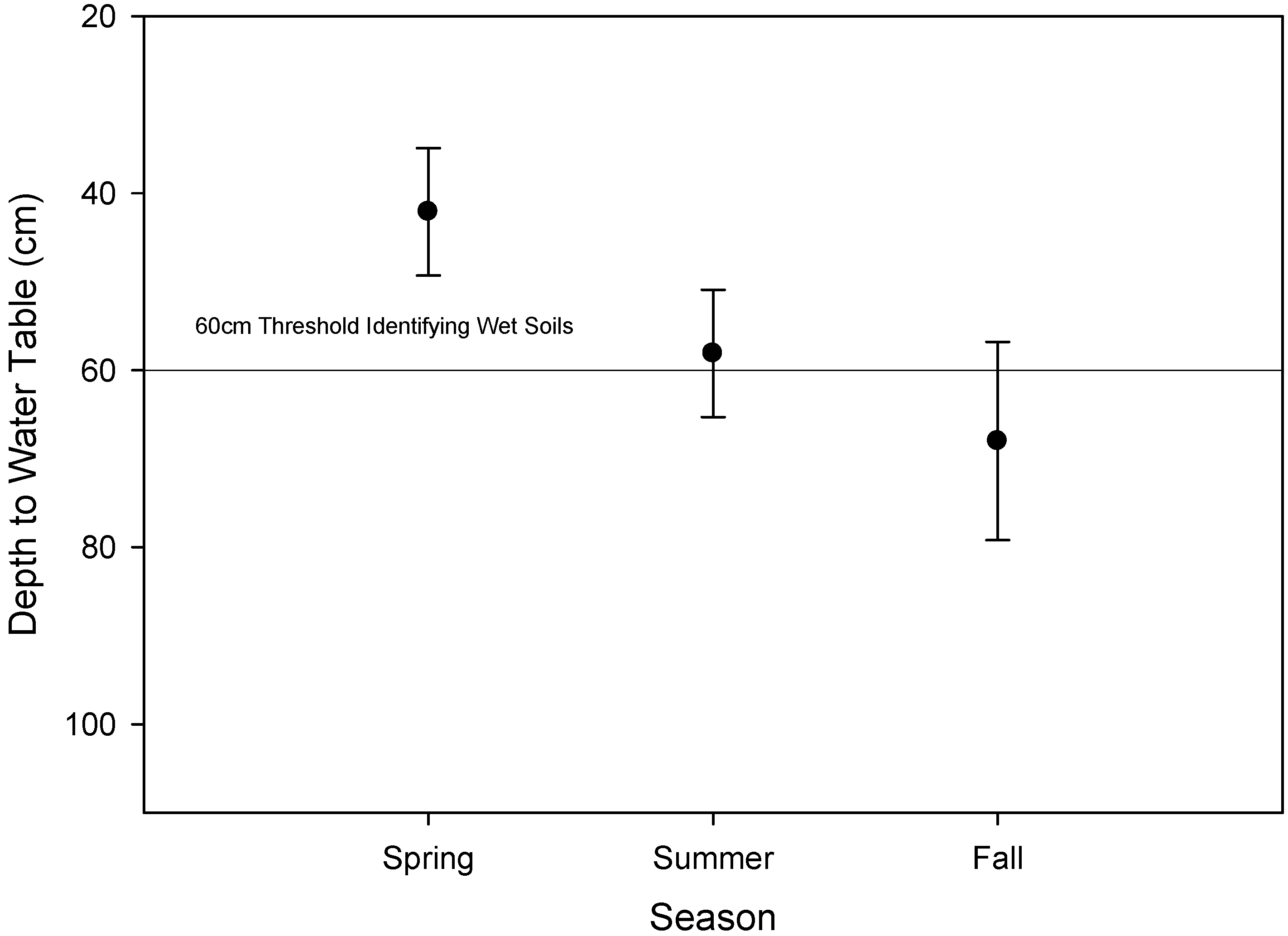
Figure 3a) and were most often above the 60 cm threshold used to identify wet locations in 2006 and 2007 combined. Summer rainfalls were higher in 2007 (309 mm) than in 2006 (154 mm), however water table trends were similar between years. As expected, spring months had shallower water table levels than the summer months (Figure 3b).
The variability of Kfs values was high within and across sites, with coefficients of variation (CV’s) ranging between 62% and 161% (Table 5). Kfs typically exhibits large spatial variability to which texture (e.g., highest Kfs in Belisle Creek–silty clay loam) and structure of soils is most directly related [38,39]. Average Kfs results were particularly high overall compared to K values published elsewhere [33,40] near the low end of saturated hydraulic range for coarse-textured soils [39]. This can be attributed to an overestimation of the α*-parameter [41]. Minimum K results appear more like actual values (Table 5). The abundant presence of silt in the sand matrix may disperse and clog up the conductive pores upon wetting.
Table 5. Comparison of saturated hydraulic conductivity (Ksat) between forested and clear-cut areas for the five selected sites. Kmean is geometric mean Kfs value, Kmax is maximum Kfs value, Kmin is minimum Kfs value, CV is coefficient of variation, and Db is soil bulk density.
Site Condition N Kmean Kmin Kmax CV Db (0–5 cm) Db (5–10 cm)
(mm h−1)(%)(Kg/m−3)(Kg/m−3)
Belisle CreekForested26508a 133268673933a §1140a
Clearcut29612a108184079972a1070a
Targe CreekForested28292a182804159990a1370a
Clearcut33115b715801341150b1380a
53km RoadForested10158a226521041084a1311a
Clearcut25144a48061611058a1315a
Cobb LakeForested25299a101680661071a1275a
Clearcut27234a831148751065a1138a
Pitka CreekForested30144a5048262940a945a
Clearcut27306a68144068960a980a
Notes: Number of measurements; Different letters following geometric mean Kfs indicate significant differences between Forested and clear-cut within the same site at P < 0.01; § Different letters following soil bulk density indicate significant differences between Forested and clear-cut within the same site at P < 0.01.
Figure 3. (a) Average water table depth at each slope location during 2006 and 2007 (least squares mean and 95% CI, n = 69) and (b) average seasonal water table depths at all locations for 2006 and 2007 (least square means and 95% CI, spring and summer n = 84, fall n = 39).
Water 05 00443 g003
There was no clear salvage logging effect on drainage patterns. Saturated soil infiltration did not show consistently lower values in cutblock areas (Table 5), possibly due to careful logging practices and large sampling error. Where compaction was evident such as at Targe Creek (i.e., lower Kfs and higher Db between 0 and 5 cm depth in the clear-cut) soil disturbance from harvesting led to poor drainage. Interestingly, the finer-texture soils at Belisle Creek had the highest rates of Kfs, which cannot be explained by texture alone since lower rates would have been expected (Table 3). At this site, the surface horizon had a loose crumb structure, which provided a very porous medium.
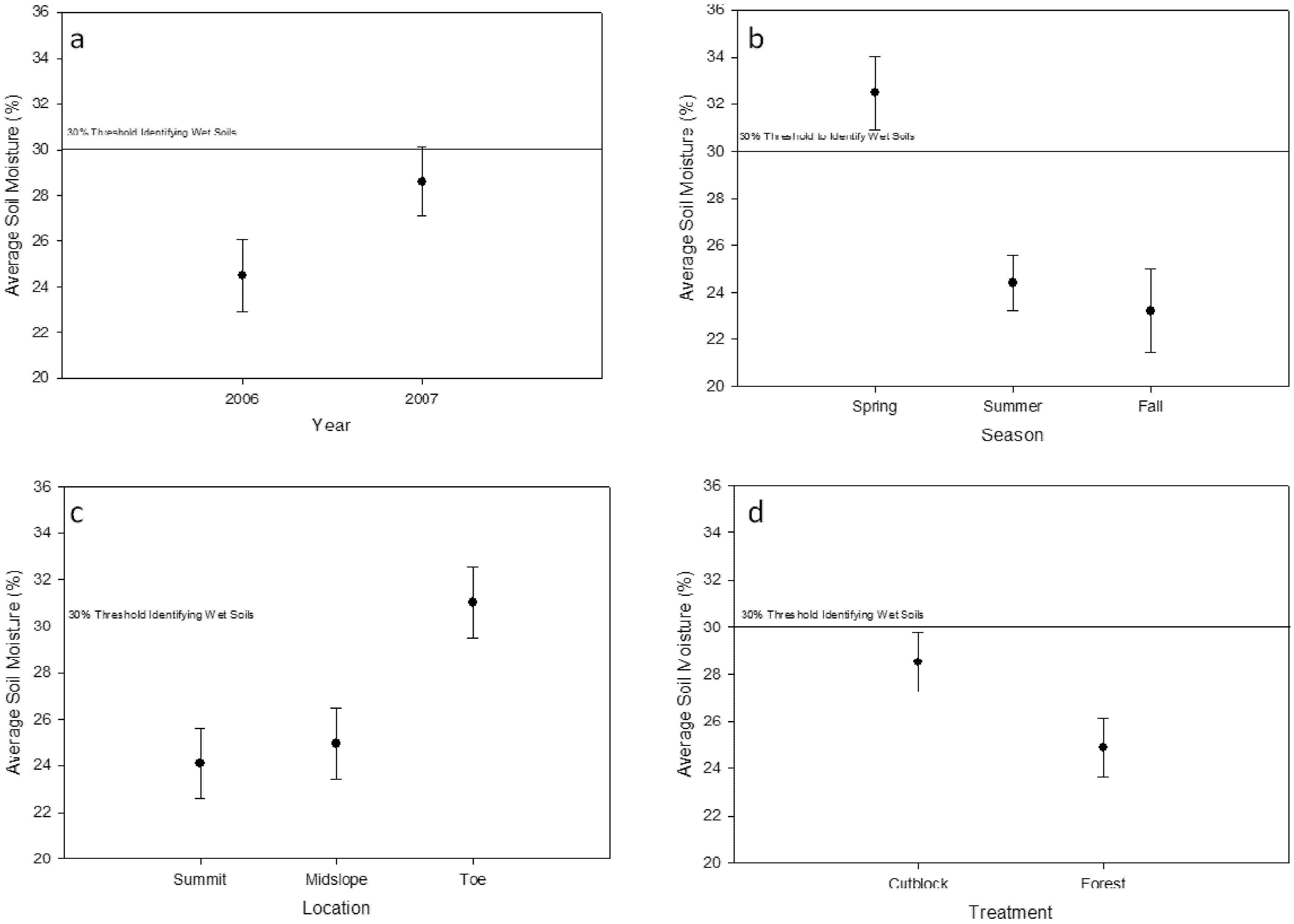
Some differences in volumetric soil moisture were observed at the qualitative assessment sites across years, treatments, slope locations, and seasons (Figure 4). Not all differences were statistically significant. Although there appears to be differences between treatments, it is not statistically significant (F1,186 = 3.86, p = 0.05). There were differences in seasons and locations (F2,186 = 11.14, p < 0.001, F1,186= 952.05, p < 0.001, respectively) with both the spring season and toe location having higher soil moisture than other seasons or slope positions. There was also a significant difference between years, with 2007 having generally higher soil moisture than 2006. This was expected because 2007 received more rainfall than 2006.
Figure 4. Average soil moisture conditions across (a) years; (b) seasons; (c) locations; and (d) treatments (Least squares means and 95% CI, n = 96). Line at 30% soil moistures identifies wet soil threshold.
Water 05 00443 g004

3.3. Post-Hoc Model Evaluation

The principal components analysis of the water table and average volumetric soil moisture content identified two groups of indicators that explained 90% and 80% of field data variability, respectively (Table 6). The general linear model (GLM) for water table and soil moisture data respectively refined this list of indicators, identifying lodgepole pine content, understory, drainage density, sensitive soils, and the topographic index as the most significant indicators. Although each GLM analysis provided an equation to predict specific values for water table or soil moisture, these formulae are not presented here because water table elevations and soil moisture cannot be predicted at the watershed scale. Instead, the equations were used to develop a new hazard prediction formula based upon the coefficient’s scale and sign (i.e., positively or negatively correlated to depth to water table or soil moisture) for each indicator. Hazard rankings were considered correct when high hazard sites were wet in both the forest and cutblock locations, moderate sites could be wet in the cutblock due to the loss in transpiration, and low sites were dry in both locations.
Table 6. Hazard indicators that were most effective at explaining data variability as identified by the principal components analysis. Note the same indicators were identified for both measurements.
MeasurementComponentIndicator
Water Table Depth1Drainage Density
Sensitive Soils
Understory
Watershed Length:Width
2Topographic index
Lodgepole Pine Cover
Soil Moisture1Sensitive Soil
Topographic Index
Relief Ratio
Drainage Density
2Lodgepole Pine Cover
In keeping with the a priori grouping of indicators, two groups were chosen for the post-hoc formula, namely the potential for increased delivery of precipitation to the forest soil and the retention of precipitation reaching the soil surface. The post-hoc hazard formula is:
Hazard = (Lodgepole Pine/Understory) × (Drainage Density/Sensitive Soils) × Topographic Index
where:
-
Lodgepole Pine: <30% cover (0.1), 30%–50% (0.3), 51%–70% (0.7), and >71% (1.0);
-
Understory: SBSdk (0.10), SBSdw3 (0.25), SBSdw2 (0.5), SBSmc3 (0.75), SBSmc2/ESSFmv1 (1.0) (SBSdk—Sub-boreal spruce dry cool, SBSdw3/2—Sub-boreal spruce dry warm, SBSmc3/2—Sub-boreal spruce moist cold, ESSFmv1—Engelmann spruce sub-alpine fire moist very cold);
-
Drainage Density: <1 km/km2 (0.1), 1–2 km/km2 (0.25), 2–3 km/km2 (0.5), 3–4 km/km2 (0.75), >4 km/km2 (1.0);
-
Sensitive Soils: 0% of watershed area with fine soils (1.0), 0–10% (0.75), 10%-20% (0.5), 20%–30% (0.75), >30% (0.1).
-
Topographic Index—dimensionless value, calculated range here is between 5 and 14 with increasing values representing a decrease in watershed slope for a given size watershed.
This formula is more hydrologically relevant than that presented for the a priori approach because it emphasizes watershed characteristics that have direct influence on net precipitation and its retention such as understory, soil type, and the relative slope of the watershed. For example, understory can lower the increase in net precipitation and also transpire [14,19], areas with less sensitive soils may have better drainage than those with sensitive soils, and the area based slope of the watershed indicates retention time of water on the soil surface [22].
Scores generated by the post-hoc formula were then ranked from one to 100 with ties receiving the same rank (i.e., 50, 51, 51, 52 were ranked 50, 51.5, 51.5, 53). High hazard sites were those with the upper 25th percentile of ranked scores (i.e., 1–25), moderate hazard watersheds were the middle 50% (26–74), and the low hazard watersheds were the lower 25th percentile of scores (75–100). In contrast to the a priori approach, the post-hoc assessment correctly identified all sites (Table 7).
High hazard watersheds had significantly shallower depth to water table at the summit across years (Figure 5, F2,57 = 5.61, p = 0.006). Harvesting effects on water table depth were not detectable as dead and dying pine stands had low transpiration due to dead pine trees as well as increased water delivery to soil more comparable to cutblock areas than to non-infested stands at toe and summit locations. High hazard sites had shallow water tables that were on average 25 cm closer to the soil surface than moderate and low hazard sites (Figure 5). Mid-slope water table was not affected by risk, season or treatment because midslope drainage is mostly controlled by gravity.
Figure 5. Average depth to water table at the summit slope location for each hazard class (error bars represent 95% CI, high n = 24, moderate n = 20, low n = 25).
Water 05 00443 g005
All toe slope sites were wet regardless of site condition and hazard. Toe slopes had shallower water table levels in spring compared to summer whereas water table levels were the same across seasons for mid-slope and summit positions. The deepest water table was recorded in the fall suggesting effects of spring runoff on toe-slope receiving areas diminished during the summer until fall precipitation replenishes the soil moisture (Figure 6).
Table 7. Watershed hazard prediction for a priori and post-hoc assessment, field data verification summary for volumetric soil moisture and water table elevation along with comments on whether the prediction was correct, over- or underestimated. Table values identify whether the average condition was wet or dry during the summer months of 2007, the wettest summer during the sample period. Post-hoc hazard prediction and hazard scores for 2007 are not included for those watersheds used to generate the post-hoc model.
Watershed a priori Hazard 2006 Post-hoc Hazard 2007 Volumetric Soil Moisture Content Forest/CutblockWater Table Elevation Forest/Cutblocka priori Prediction Post-hoc Prediction
Peta CreekLowLowN/AdryCorrectCorrect
Angly LakeLowN/A *N/AdryCorrectN/A
10573ModerateLowdry/dryN/ACorrectCorrect
Pitka CreekLowLowN/Adry/dryCorrectCorrect
ShaydeeLowN/Adry/dryN/ACorrectN/A
10330LowN/Adry/dryN/ACorrectN/A
10557HighN/Adry/wetN/AOverestimateN/A
Crystal LakeHighModerateN/AdryOverestimateCorrect
Chowsunkut LakeHighModerateN/Adry/dryOverestimateCorrect
Belisle CreekHighModerateN/Adry/dryOverestimateCorrect
10485HighN/Adry/dryN/AOverestimateN/A
10610ModerateModeratedry/dryN/ACorrectCorrect
10411ModerateN/Awet/wetN/AUnderestimateN/A
Targe CreekModerateHighN/Awet/wetUnderestimateCorrect
Targe Creek-44ModerateHighwet/wetwet/wetUnderestimateCorrect
10426HighN/Adry/wetN/AOverestimateN/A
Cobb LakeLowHighN/Awet/wetUnderestimateCorrect
Note: * N/A These sites were used to build the post-hoc model.
Figure 6. Seasonal average depth to water table at toe slope locations (error bars represent 95% CI, n = 27 spring and summer n = 13 for fall).
Water 05 00443 g006
The analysis of ln-transformed Kfs from all sites indicated a statistically significant effect on watershed hazard (F3,256 = 4.10, p = 0.007) and site condition (F5,254 = 3.71, p = 0.003). Highest measured hydraulic conductivities were found in the high hazard forested sites. In contrast, moderate hazard clear-cut area had the lowest Kfs but soil disturbance was not observed. Great variability in Kfs in part due to very high spatial variability in soil properties may explain this result. Based on our sampling, harvesting did not lead to a significant reduction in Kfs across watershed hazard. There was faster surface drainage in the high hazard MPB areas than in the low hazard MPB areas. This indicates that differences in Kfs may not be explained by high water table levels, which are less likely to occur where surface drainage is fast. Hard almost cemented layers less than 60 cm deep were observed during soil pit excavation at some high and moderate hazard sites (e.g., Targe Creek, watersheds 10557 and 10426) that may impede drainage similar to that observed in Ortstein layers [42]. Although not impervious to water, the naturally compacted layer has a slower percolation rate that may be inadequate to drain large quantities of water reaching the soil in stands with a dead pine overstory or large salvage harvested areas. Under these conditions, soil saturation persists longer after spring runoff and a large summer storm can quickly fill up available storage in the soil profile raising the water table quickly, which may impede forest management activities.
The influence of pre-existing conditions in the soil profile such as a moist and soft layer lying over a dry or hard subsurface layer can be exacerbated by compaction [43] and may result in a higher hazard for salvage-logged areas. For example, there was a statistically significant relationship between site condition and Kfs (p < 0.01) at Targe Creek (Table 5). Compaction was evident in the clear-cut sampling areas and sample sites showed a significant increase in bulk density in the top 5 cm of soil following skidding (Table 5). These compacted areas were characterized by a platy structure and loss of original structure [44]. The reduction in large pore space in the clear-cut, which is responsible for most of the saturated flow, produced an average Kfs rate of 115 mm h−1), which represented a reduction of 57% in Kfs from the MPB forest. Harvesting operations and subsequent soil compaction can decrease field saturated hydraulic conductivity [45].

4. Conclusions

This project developed a field-verified watershed level hydrologic hazard assessment procedure to assess the relative hazard of experiencing wet soils during salvage logging of MPB-affected forests in the Vanderhoof Forest District. Watering-up occurred in response to precipitation in watersheds with characteristics that increase net precipitation and retention of that precipitation such as dominant forest stand cover of dead pine trees, lack of understory, low watershed slope, and fine textured soils. Findings indicate that salvage logging did not influence water table elevations or soil moisture when compared to standing beetle-killed stands but it did increase soil compaction, which can alter drainage pattern and efficiency. Although the model presented here was developed for the Vanderhoof Forest District, some model components may be transferrable to other areas experiencing a forest pest outbreak or other watershed-level disturbance. Similarly, the model-development process presented here is suitable for transfer to other areas requiring a watershed-level hazard analysis for increase in soil moisture.

Acknowledgments

The authors would like to thank Phillip Krauskopf, Maria Fe Saraiva, Megan Campbell, Cindy Chevalier and Amy Barnes for field support.

References

  1. Carroll, A.L.; Taylor, S.W.; Régnière, J.; Safranyik, L. Effect of Climate Change on Range Expansion by the Mountain Pine Beetle in British Columbia. In Mountain Pine Beetle Symposium: Challenges and Solutions, 30–31 October 2003; Information Report BC-X-399; Shore, T.L., Brooks, J.E., Stone, J.E., Eds.; Natural Resources Canada: Victoria, Canada, 2003; pp. 223–232. [Google Scholar]
  2. Taylor, S.W.; Carroll, A.L. Disturbance, Forest Age, and Mountain Pine Beetle Outbreak Dynamics in BC: A historical perspective. In Mountain Pine Beetle Symposium: Challenges and Solutions, 30–31 October 2003; Information Report BC-X-399; Shore, T.L., Brooks, J.E., Stone, J.E., Eds.; Natural Resources Canada: Victoria, Canada, 2003; pp. 41–51. [Google Scholar]
  3. Safranyik, L.; Carroll, A.L. The Biology and Epidemiology of the Mountain Pine Beetle in Lodgepole Pine Forests. In The Mountain Pine Beetle: A Synthesis of Biology, Management and Impacts on Lodgepole Pine; Safranyik, L., Wilson, B., Eds.; Natural Resources Canada, Canadian Forest Service, Pacific Forestry Centre: Victoria, Canada, 2006; pp. 3–66. [Google Scholar]
  4. Bethalmy, N. A Colorado episode: Beetle epidemic, ghost forests, more streamflow. Northwest Sci. 1975, 49, 95–105. [Google Scholar]
  5. Putz, G.; Burke, J.M.; Smith, D.W.; Chanasyk, D.S.; Prepas, E.E.; Mafumo, E. Modelling the effects of boreal forest landscape management upon streamflow and water quality: Basic concepts and considerations. J. Environ. Eng. Sci. 2003, 2, S87–S101. [Google Scholar] [CrossRef]
  6. Tokuchi, N.; Ohte, N.; Hobara, S.; Kim, S.J.; Masanori, K. Changes in biogeocemical cycling following forest defoliation by pine wilt disease in Kiryu experimental catchment in Japan. Hydrol. Process. 2004, 18, 2727–2736. [Google Scholar] [CrossRef]
  7. Dunne, T.; Leopold, L.B. Interception. In Water in Environmental Planning; W.H. Freeman & Company: New York, NY, USA, 1978; pp. 83–94. [Google Scholar]
  8. Spittlehouse, D.L. Sap Flow and Transpiration of Old Lodgepole Pine Trees. In Proceedings of 25th Conference on Agricultural and Forest Meterology, Norfolk, VA, USA, 20–24 May 2002; pp. 123–124.
  9. Banner, A.; Mackenzie, W.; Haeussler, S.; Thomson, S.; Pojar, J.; Trowbridge, R. A Field Guide to Site Identification and Interpretation for the Prince Rupert Forest Region; Handbook No. 26; Ministry of Forests: Victoria, Canada, 1993. [Google Scholar]
  10. Knight, D.H.; Fahey, T.J.; Running, S.W. Water and nutrient outflow from contrasting lodgepole pine forests in Wyoming. Ecol. Mono. 1985, 55, 29–48. [Google Scholar] [CrossRef]
  11. Dubé, S.; Plamondon, A.P. Relative importance of interception and transpiration changes causing watering-up after clearcutting on four wet sites. In Proceedings of Man’s Influence on Freshwater Ecosystems and Water Use; Petts, G., Ed.; IAHS Press: Boulder, CO, USA, 1996; pp. 113–120. [Google Scholar]
  12. Boon, S. Snow accumulation and ablation is a beetle-killed pine stand in Northern Interior British Columbia. B. C. J. Ecosyst. Manag. 2007, 8, 1–13. [Google Scholar]
  13. Plamondon, A.P. Forest Harvesting Effects on Water Yield and Water Quality; Faculty Member Report; University Laval: Québec, Canada, 1993. [Google Scholar]
  14. Brown, M. The Carbon, Water and Energy Balances of Two Lodgepole Pine Stands Recovering from Mountain Pine Beetle Attack in British Columbia. Ph.D. Thesis, Faculty of Graduate Studies (Soil Science), University of British Columbia, Vancouver, Canada, April 2011. [Google Scholar]
  15. Dubé, S. Watering-up after clearcutting on forested wetlands of the St Lawrence lowland. Master’s Thesis, School of Graduate Studies, University of Laval, Québec, Canada, March 1994. [Google Scholar]
  16. Potts, D.F. Hydrologic Impacts or a large-scale mountain pine beetle epidemic. Water Resour. Bull. 1984, 20, 373–377. [Google Scholar]
  17. Sun, G.; McNulty, S.G.; Shepard, J.P.; Amatya, D.M.; Riekerk, H.; Comeford, N.B.; Skaggs, W.; Swift, L., Jr. Effects of timber management on the hydrology of wetland forests in the southern United States. For. Ecol. Manag. 2001, 143, 227–236. [Google Scholar]
  18. Lindenmayer, D.; Burton, P.J.; Franklin, J.F. Salvage Logging and its Ecological Consequences; Island Press: Washington, DC, USA, 2008. [Google Scholar]
  19. Schmid, J.M.; Mata, S.A.; Martinez, M.H.; Troendle, C.A. Net Precipitation within Small Group Infestations of the Mountain Pine Beetle; USDA Forest Service, Rocky Mountain Forest and Range Experiment Station: Fort Collins, CO, USA, 1991. [Google Scholar]
  20. Coates, D.K.; DeLong, C.; Burton, P.J.; Sachs, D.L. Report for the Chief Forester August 2006: Abundance of Secondary Structure in Lodgepole Pine Stands Affected by the Mountain Pine Beetle. Available online: http://www.for.gov.bc.ca/hfp/mountain_pine_beetle/stewardship/report.pdf (accessed on 15 January 2013).
  21. Knighton, D. Drainage Networks. In Fluvial Forms and Processes: A New Perspective, 2nd ed; Arnold Publishers: London, UK, 1998; pp. 8–64. [Google Scholar]
  22. Hewlett, J.D. Drainage Basin Morphology. In Principles of Forest Hydrology; University of Georgia Press: Athens, GA, USA, 1982; pp. 16–24. [Google Scholar]
  23. Berger, K.P.; Entekhabi, D. Basin hydrologic response relations to distributed physiographic descriptors and climate. J. Hydrol. 2001, 247, 169–182. [Google Scholar]
  24. Manly, B.F.J. Principal Components Analysis, Mutivariate Statistical Methods: A Primer, 2nd ed; Chapman & Hall/CRC: Boca Raton, FL, USA, 1994; pp. 76–92. [Google Scholar]
  25. Dingman, S.L. Stream Response to Water-Input Events. In Physical Hydrology, 2nd ed; Waveland Press, Inc.: Long Grove, IL, USA, 2002; pp. 389–456. [Google Scholar]
  26. Hjerdt, K.N.; McDonnell, J.J.; Seibert, J.; Rodhe, A. A new topographic index to quantify downslope controls on local drainage. Water Resour. Res. 2004, 40. [Google Scholar] [CrossRef]
  27. Starr, J.L.; Paltineau, I.C. Methods for Measurement of Soil Water Content: Capacitance Devices. In Methods of Soil Analysis: Part 4 Physical Methods; Book Series No. 5; Soil Science Society of America: Madison, WI, USA, 2002; pp. 463–474. [Google Scholar]
  28. Cobos, D.R.; Chambers, C. Calibrating ECH20 soil moisture sensors. Application Note, Decagon Devices Inc. 2009. Available online: http://www.decagon.com/assets/Uploads/13393-04-CalibratingECH2OSoilMoistureProbes.pdf (accessed on 15 January 2013).
  29. Pennock, D.J.; Anderson, D.W.; de Jong, E. Landscape-scale changes in indicators of soil quality due to cultivation in Saskatchewan, Canada. Geoderma 1994, 64, 1–19. [Google Scholar]
  30. Weight, W.D.; Sonderegger, J.L. Basic Geophysics of the Shallow Subsurface. In Manual of Applied Field Hydrogeology; McGraw-Hill: New York, NY, USA, 2001; pp. 121–164. [Google Scholar]
  31. Dubé, S.; Plamondon, A.; Rothwell, R. Watering-up after clear-cutting on forested wetlands of the St. Lawrence lowland. Water Resour. Res. 1995, 31, 1741–1750. [Google Scholar] [CrossRef]
  32. Carnell, R.; Anderson, M.A. A technique for extensive field measurement of soil anaerobism by rusting of steel rods. Forestry 1986, 59, 129–140. [Google Scholar]
  33. Bagarello, V.; Iovino, M.; Elrick, D. A simplified falling-head technique for rapid determination of field-saturated hydraulic conductivity. Soil Sci. Soc. Am. J. 2004, 68, 66–73. [Google Scholar] [CrossRef]
  34. Elrick, D.E.; Reynolds, W.D. Infiltration from Constant-Head Well Permeameters and Infiltrometers. In Advances in Measurement of Soil Properties: Bringing Theory into Practice; Topp, G.C., Reynolds, W.D., Green, R.E., Eds.; Soil Science Society of America: Madison, WI, USA, 1992; pp. 1–24. [Google Scholar]
  35. Gee, G.W.; Bauder, J.W. Particle-Size Analysis. In Methods of Soil Analysis. Part 1, 2nd; Klute, A., Ed.; Agronomy Monograph 9; American Society of Agronomy—Soil Science Society of America: Madison, WI, USA, 1986; pp. 383–411. [Google Scholar]
  36. Block, R.; Van Rees, K.C.J.; Pennock, D.J. Quantifying harvesting impacts using soil compaction and disturbance regimes at a landscape scale. Soil Sci. Soc. Am. J. 2002, 66, 1669–1676. [Google Scholar] [CrossRef]
  37. Culley, J.L.B. Density and Compressibility. In Soil Sampling and Methods of Analysis; Carter, M.R., Ed.; Lewis Publishers: Boca Raton, FL, USA, 1993; pp. 529–539. [Google Scholar]
  38. Kutilek, M. Soil hydraulic properties as related to soil structure. Soil Tillage Res. 2004, 79, 175–184. [Google Scholar] [CrossRef]
  39. Hillel, D. Environmental Soil Physics; Elsevier: San Diego, CA, USA, 1998. [Google Scholar]
  40. Sanjit, K.D.; Shukla, M.K. Variability of hydraulic conductivity due to multiple factors. Am. J. Environ. Sci. 2012, 8, 489–502. [Google Scholar]
  41. Bagarello, V.; Provenzano, G. Factors affecting field and laboratory measurement of saturated hydraulic conductivity. Trans. ASAE 1996, 39, 153–159. [Google Scholar]
  42. Lambert, J.L.; Hole, F.D. Hydraulic properties of an Ortstein horizon. Soil Sci. Soc. Am. J. 1971, 35, 785–787. [Google Scholar] [CrossRef]
  43. Batey, T. Soil compaction and soil management—A review. Soil Use Manag. 2009, 25, 335–345. [Google Scholar] [CrossRef]
  44. BC Ministry of Forests, Soil Conservation Surveys Guidebook; Forest Practices Code of British Columbia Guidebook, 2nd ed; Forest Practices Branch, BC Ministry of Forests: Victoria, BC, Canada, 2001.
  45. Startsev, A.D.; McNabb, D.H. Effects of skidding on forest soil infiltration in west-central Alberta. Can. J. Soil Sci. 2000, 80, 617–624. [Google Scholar] [CrossRef]

