1. Introduction
Current stormwater tank design criteria have not yet been consolidated in engineering practice to address the complexity of their functioning model, particularly pollutant characterization.
In the last decades the concept of environmental water management is increased among the urban water resource managers and so actions, such as stormwater tanks, which have multiple benefits, are increasingly being built into urban water sewer system. It is really important therefore that the accuracy of commonly used models is understood and verified [
1].
Many authors have conducted sensitivity analysis aimed at defining stormwater tank efficiency using various configurations. The efficiency of a stormwater tank is evaluated in terms of total suspended solids (TSS) mass and of water storage discharged to the receiver. De Martino
et al. [
2,
3] evaluated the efficiency of an on-line and capture stormwater tank and compared the results to an off-line system. Calabrò & Viviani [
4] developed the numerical model COSMOSS to perform continuous simulations to test the effectiveness of both capture and on-line tanks. They concluded that capture tanks, with equal performance, require smaller accumulation storage.
Each tank type can have different management rules, such as varying the emptying mode, and this feature influences the system efficiency in terms of both pollutant quantity and water volumes sent to the receiving water body.
Todeschini
et al. [
5] analyzed the management of an off-line tank and concluded that an intermittent operation is more advantageous in terms of volume delivered to treatment compared to an on-line tank with continuous emptying.
Paoletti [
6] examined three management rules for stormwater tanks and concluded that the preferred management rule is the one in which the tank is flooded for each event and emptying begins after the tank is filled. This rule has several disadvantages: if the tank is not full at the end of an event, a foul odor is possible and sedimentation in the tank can reduce capacity while waiting for the next event [
6]. Consequently, it is better to manage the tank such that it is emptied (after a fixed time at the end of each flooding event) without waiting for the complete filling. This management rule was also considered by Balistrocchi
et al. [
7], who fixed the time to wait to empty the tank as equal to the period in which rain did not occur, after which, a new meteorological event is considered independent from the previous one (inter-event time definition, IETD). To set the tank configuration and management mode, it is necessary to choose an approach to model the tank management. Two numerical approaches are typically followed: numerical continuous simulation and a semi-probabilistic approach. The first approach uses specific software to solve the equations of motion and to simulate the pollutant accumulation and removal. This approach allows the operation of a stormwater tank to be simulated once all of the catchment characteristics are defined and a rainfall event is assigned. Several authors have used this approach to estimate stormwater tank efficiency for case study basins with fixed characteristics and subject to specific rainfall patterns [
2,
3,
4].
In the semi-probabilistic approach, the rainfall is characterized by a probability distribution function (pdf) to estimate stormwater tank efficiency. Several applications have assumed that the synthetic meteorological variables of the duration, volume, and dry time of rain can be represented by an exponential distribution with one parameter [
8,
9,
10,
11,
12]. Balistrocchi
et al. [
7] proposed a semi-probabilistic model based on the use of the Weibull pdf with a non-zero lower limit for the description of the rain event volume, combined with a two-parameter model of gross rain purification. The authors [
7], referring to the M (V) curves that correlate the discharged fluid volume to the pollution load proposed by Bertrand-Krajewski
et al. [
13], derived a semi-probabilistic model of water quality similar to that for precipitation.
All the previous cited works published in prestigious international journals, have been widely used as a reference in the technical literature of stormwater tanks.
This paper compares the efficiency values calculated from the continuous simulation approach by assuming four different capture tank operational modes. Subsequently, a semi-probabilistic approach is applied to one of the operational settings to highlight the differences from the continuous simulations. The studied approaches provide very comparable results. Nevertheless, both of them require a series of rainfall data, which is not always available, with a time interval not exceeding 15 min, taking into account the characteristics of the urban catchments.
2. Comparison of Management Practices for Capture Tanks
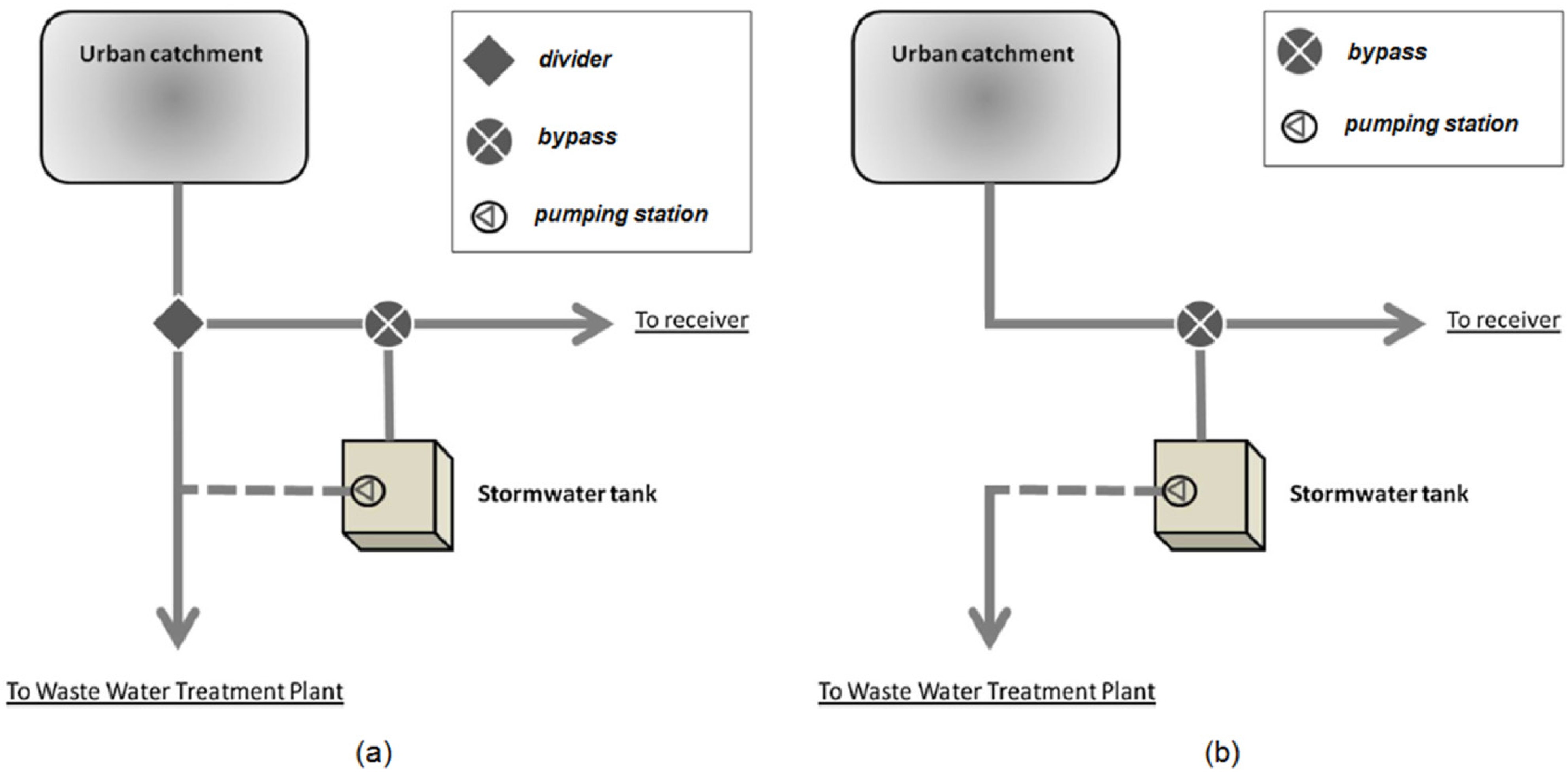
The choice of a stormwater capture tank (
Figure 1) operational mode can have a significant influence on the tank’s efficiency. First, it is necessary to differentiate between the operation of a tank-only and bypass-tank system. Then, the tank management, namely, the emptying operation generally conducted at a pumping station, must be considered.
Figure 1.
Capture tank operation layout. (a) With a divider; (b) Without a divider.
Figure 1.
Capture tank operation layout. (a) With a divider; (b) Without a divider.
This paper compares the performance of the four different tank configurations (A–D) described below.
In configuration A, which was used for simulations in several previous works [
2,
3], there is initially a divider (
Figure 1a) for a flow threshold equal to five times the average dry weather flow (5Q
mn, with Q
mn = 2 lps). If exceeding this value, excess flow fills the tank (if it is not full) by means of a bypass device; otherwise, it is sent to the receiving water body. The tank is pumped empty at the end of the event at a flow rate of 3Q
mn. The pump stops if the tank is empty or the input flow rate exceeds 2Q
mn to ensure that the flow rate sent to treatment is not higher than the limit value of 5Q
mn.
Configuration B is the same as A (
Figure 1b) but without a divider. Therefore, the flow coming from upstream is directly conveyed to the tank. The management procedures outlined above are followed.
Configuration C (
Figure 1b), which was also analyzed by Balistrocchi
et al. [
7] and Paoletti [
6], is based on the definition of a storm “event” as the sum of a wet and a dry period, where the dry period is not shorter than a fixed interevent time definition (IETD). This duration can be defined as the minimum dry weather period that allows to separate two subsequent rainfall pulses into statistical independent storms.
It is common practice to distinguish independent events, such as the absence of a rainfall period (or lack of flow in the network), after which a new meteorological event is considered independent from the previous event. In this case, the tank is filled if it is empty, and it is emptied using a pump [with a flow rate equal to V/haimp/(IETD/2), where (V/haimp) is the specific tank capacity] if the maximum level is reached or if, even if not full, the time between rainfall events is equal to IETD/2.
In configuration D (
Figure 1b), emptying is active if either the tank is full or there is an elapsed dry time of IETD/2. Emptying occurs at a flow rate of V/ha
imp/(IETD/2), and additional water volume is not allowed. If the meteorological event is not complete; a dry period equal to IETD is required before the tank is available again. Configuration D differs from configuration C because the tank may be filled only once during a single event, and thus, once the first volume of rain is collected, it empties to receive those of the next event.
3. Numerical Continuous Simulation
To compare the four modes of management, it is useful to refer to the following tank efficiency indexes [
3]:
where M
r and W
r are the total suspended solids (TSS) mass and the water storage discharged to the receiver, respectively; and M
b and W
b are the mass and storage input to the system, respectively.
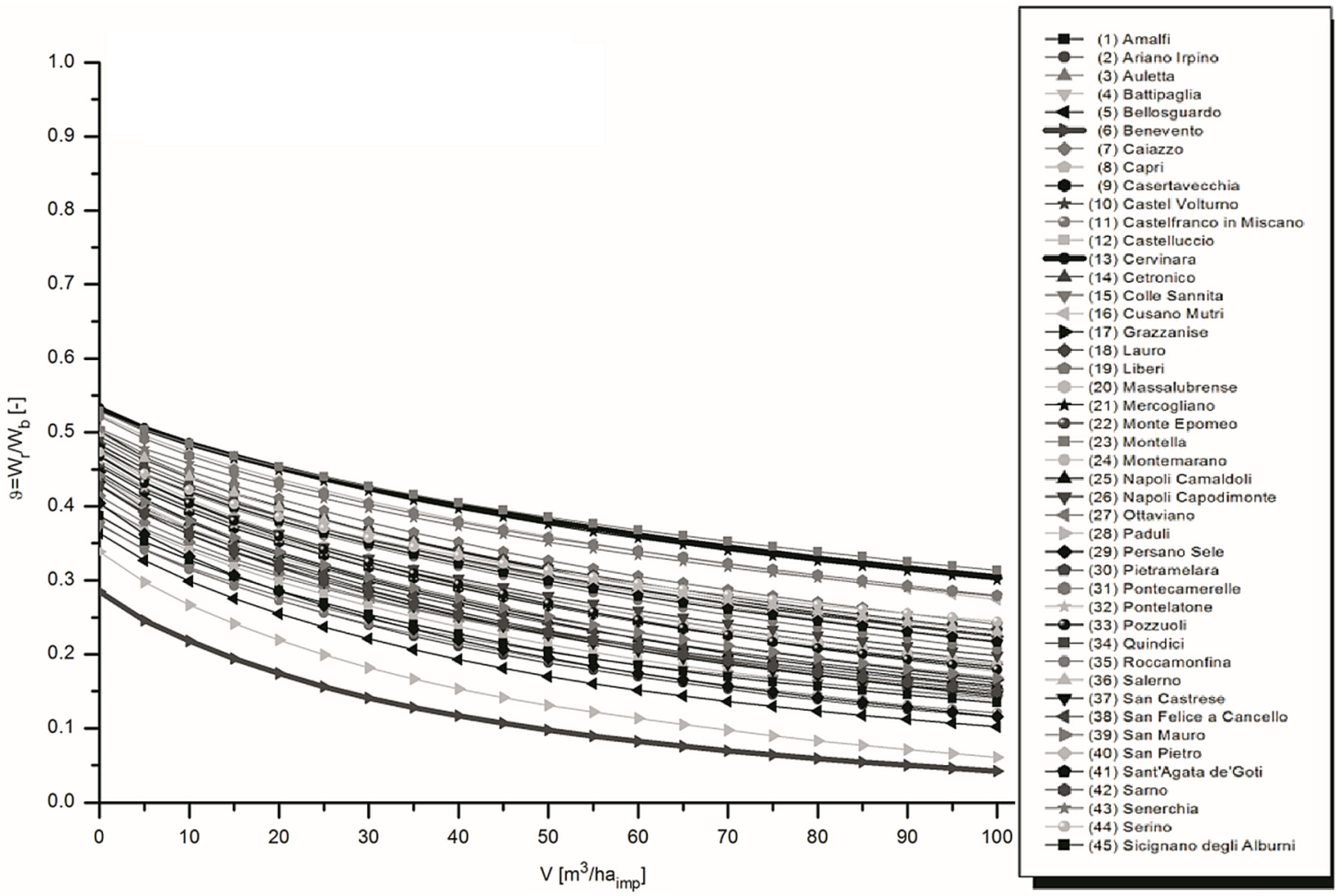
The comparison considers a virtual catchment with average urban characteristics of south Italy. This study considers two weather rain gauge stations in the Campania region (Benevento and Cervinara), which are among the 45 stations considered in the work of De Martino
et al. [
3]. These two were chosen because they represent extreme behavior in terms of stormwater efficiency. In observing the trend of θ with tank storage volume in
Figure 2, it is evident that the curves for the two gauge stations chosen are consistent with all of the other stations. Similar results are shown in the graph related to η [
3], not shown here for the sake of brevity.
Continuous simulations were performed using the EPA StormWater Management Model (SWMM 5) [
3]. Simulations were carried out referring to a drainage system within a virtual Italian urban catchment. The main features of the catchment are shown in
Table 1 and include the following parameters: catchment area and width, average surface slope, percentage of impervious area Manning coefficient for pervious and impervious surfaces, and depth of depression storage on pervious (d
p-perv.) and impervious (d
p-imp.) surfaces. Overflow pollution was calculated referring to TSS mass and concentration since they are strictly correlated with other common urban pollutants (BOD5, COD, heavy metals), as many experimental researches have shown [
2,
3]. Further details are reported in previous work cited [
2,
3].
Table 1.
Characteristics of the virtual catchment analyzed.
Table 1.
Characteristics of the virtual catchment analyzed.
| Area | Catchment width | Slope | Impervious surface | nperv | nimp | dp-perv. | dp-imp. |
|---|
| 4 ha | 150 m | 0.50% | 75% | 0.040 s/m1/3 | 0.025 s/m1/3 | 5 mm | 1 mm |
Figure 2.
Volumes discharged into the receiver with varying useful tank storage. The characteristics of the two rain gauge stations considered are provided in
Table 2.
Figure 2.
Volumes discharged into the receiver with varying useful tank storage. The characteristics of the two rain gauge stations considered are provided in
Table 2.
Table 2.
Characteristics of the rainfall series analyzed.
Table 2.
Characteristics of the rainfall series analyzed.
| Stations | Available data sets | Time step | Mean annual rainfall depth |
|---|
| Benevento | 1 August 1998–31 August 2009 | 10 min | 573 mm |
| Cervinara (CE) | 17 October 2000–31 August 2009 | 10 min | 1601 mm |
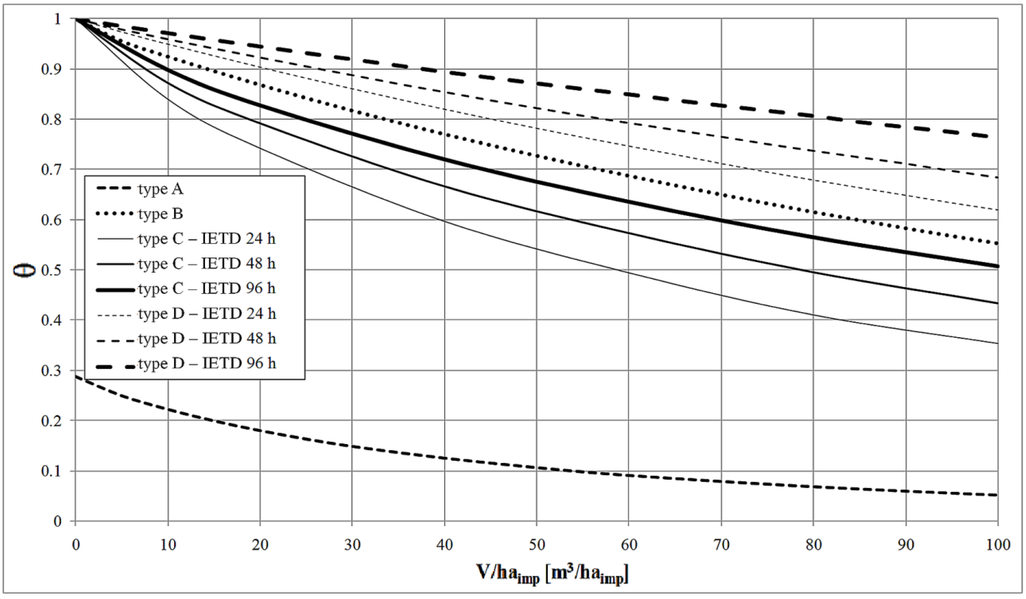
Figure 3 presents the trend of the efficiency index θ for the four different types of capture tank considered. The three IETD values for types C and D were fixed, equal to 24, 48, and 96 h, similar to the values considered by other authors [
6,
7].
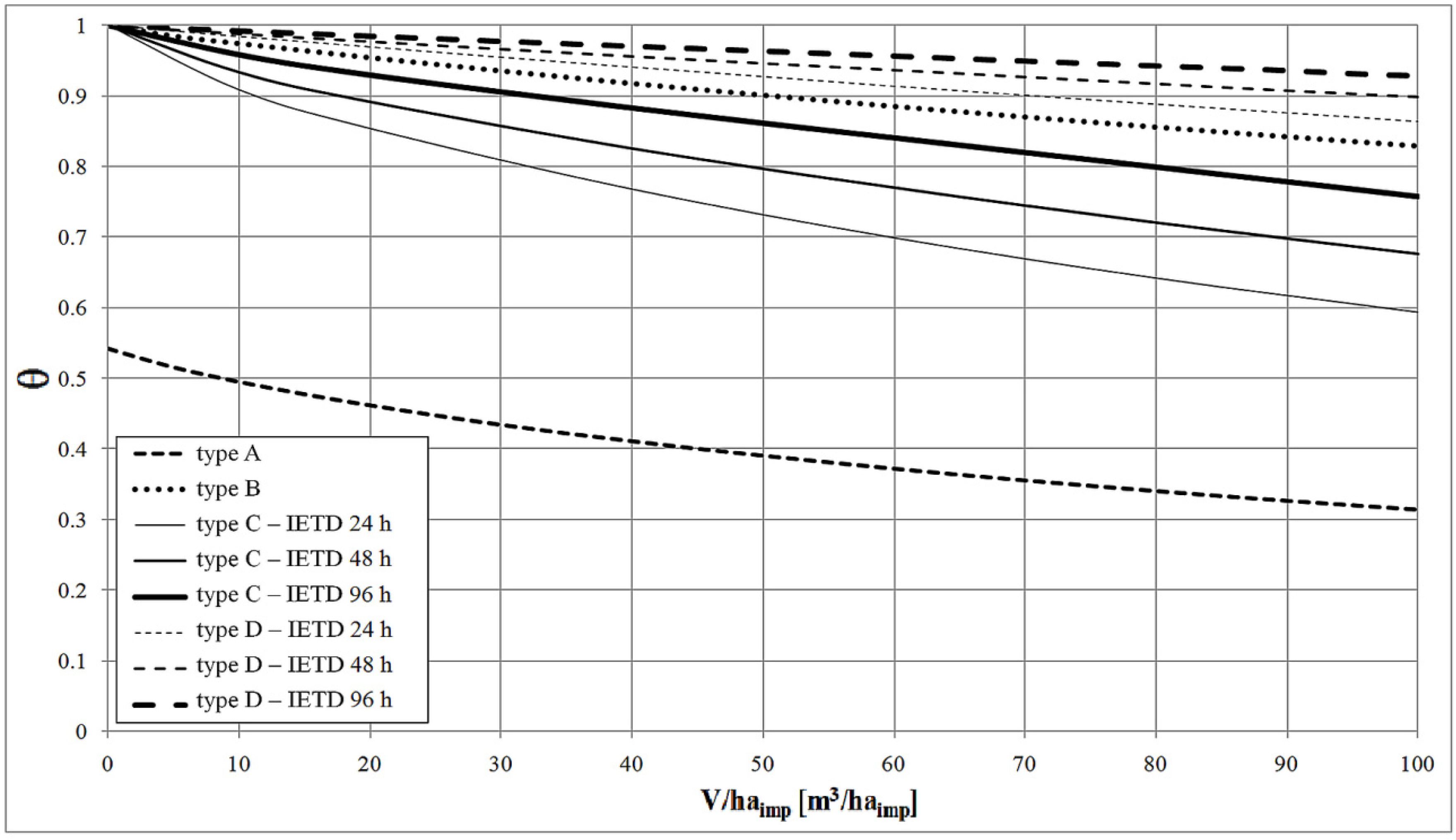
Figure 4 presents the corresponding information for the station at Cervinara.
Figure 3.
Benevento station. Efficiency index θ compared to tank storage V/haimp, varying from 0 to 100 m3/haimp.
Figure 3.
Benevento station. Efficiency index θ compared to tank storage V/haimp, varying from 0 to 100 m3/haimp.
Figure 4.
Cervinara station. Efficiency index θ compared to tank storage V/haimp, varying from 0 to 100 m3/haimp.
Figure 4.
Cervinara station. Efficiency index θ compared to tank storage V/haimp, varying from 0 to 100 m3/haimp.
For both scenarios, configuration A is significantly more efficient than the other configurations in terms of water volume sent to the receiver (the θ value is smaller) because of the presence of the bypass, which allows for the removal of a large part of the volume coming from upstream before the tank is flooded. Once the threshold is exceeded, the tank’s accumulation capability can be exploited. The absence of the bypass in the other tank types results in an increase of θ. In particular, the following observations can be made:
Configuration D has the lowest storage efficiency of the tank types considered. The tank achieves maximum θ values, decreasing with the IETD. As the IETD decreases, the pump flow, which is necessary to empty the tank, increases (equal to the tank storage divided by IETD/2), enabling the tank to repeatedly be ready to capture the volumes of water arriving from upstream;
Configuration C displays smaller θ values than the other configurations with a tank alone, and the values decrease with increasing IETD, for the same reason provided above;
Configuration B exhibits an efficiency behavior between C and D.
In configuration C, less volume is sent to the receiver compared to B and D because of different pump management protocols. For configuration B, emptying is only activated if the flow coming from upstream is zero, and it stops if this condition no longer exists, or if the tank is empty. Thus, the tank can be filled only once for each event. This situation also occurs for configuration D; it is emptied if full and fills again after a period equal to dry IETD. These two types differ because the first (B) is emptied as soon as the event ends and becomes immediately available to the reservoir, whereas the second (D) provides for a non-operating period. The lifting capacity in B is constant at 5 Qmn, whereas it varies according to the tank storage in D.
Configuration B achieves higher efficiency values (lower θ values) than D because it does not require the time span equal to the dry IETD to operate again, and in the investigated configurations, the flow rate of emptying is 5 Qmn, which is higher than the flow rates in D. Thus, the tank is available more frequently to send new volume to the receiver.
In configuration C, if the tank is full, the emptying is activated and the storage capacity is again available, even during the same rain event. In this manner, particularly for long-lasting events and for configurations B and D, once the tank capacity is exhausted, it does not operate; in configuration C, the tank may be filled and emptied during the cycle, sending larger volumes to the receiver.
Configuration C, with a low IETD, exhibits higher efficiency than configuration B and thus also D.
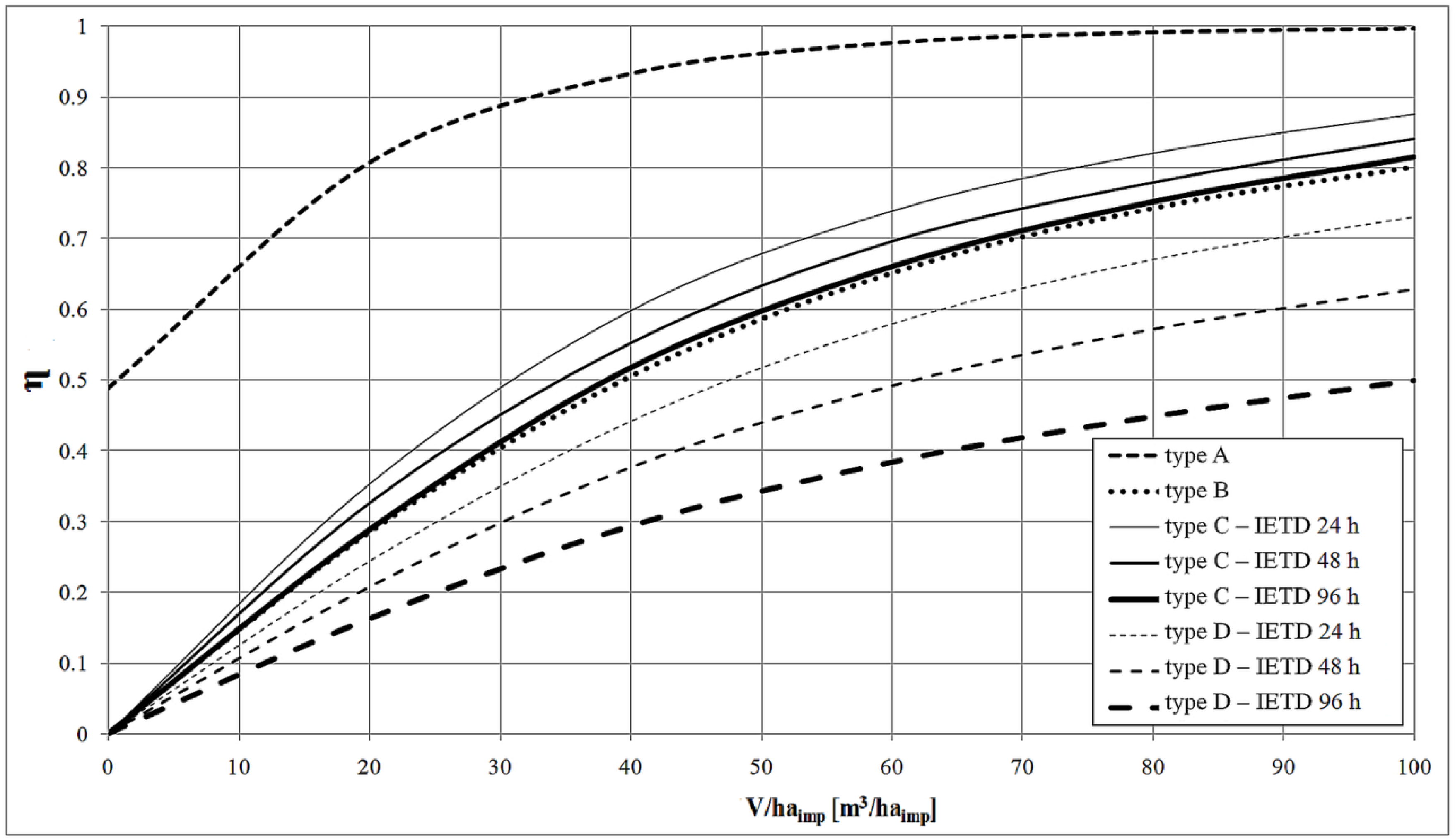
Efficiency varies with the mass of pollutant spilled into the receiver. The trend of the efficiency index η is shown in
Figure 5 for the Cervinara station; similar results were found in the Benevento station but are not reported for the sake of brevity.
The curve analysis reveals the following:
Configuration A exhibits the highest efficiency because of the combined bypass-tank system;
Configuration C has the maximum efficiency among the solutions with a tank-only system, and the efficiency increases with decreasing IETD;
The relative efficiency of configuration B is intermediate. The relative curve in
Figure 5 is placed between the C and D curves;
Configuration D exhibits smaller values of η, which decrease with increasing IETD.
The simulations indicate that the volume delivered to the treatment increases as the pollutant mass removed from the water body receiver increases. Therefore, among the tank-only systems, configuration C, which sends more volume to the receiver, also removes more mass pollutants, and is thus more efficient.
However, the volumes accumulated in configuration C, compared to B and D, are from the central or final period of the rain event, which typically implies a lower pollutant content than present at the beginning of the event. In practice, C is as efficient as B for a large volume. This result is also evident by comparing the curve of θ related to C-IETD 96 h, for example, which differs from the curve for B (
Figure 4); the same trend is not observed in the η curves (
Figure 5). Furthermore, B has significant operational advantages because the material that is delivered does not remain in the tank for a long time, avoiding foul odors and sedimentation deposits, along with a possible reduction of capacity and pumping station malfunctioning, as occurs in C.
Figure 5.
Cervinara station. Efficiency index η compared to tank storage V/haimp, varying from 0 to 100 m3/haimp.
Figure 5.
Cervinara station. Efficiency index η compared to tank storage V/haimp, varying from 0 to 100 m3/haimp.
The results described above were achieved using the continuous simulation approach. In the following section, the semi-probabilistic model is discussed, as reported in Bacchi
et al. [
8], with reference to the tank-only system with the highest efficiency rating (C).
4. Semi-Probabilistic Approach to Evaluate the Capture Tank Efficiency
The semi-probabilistic approach was used just to make a comparison with numerical continuous simulations in a context (southern Italy) significantly different from those analyzed in different paper.
To apply this approach, it is necessary to reconstruct the series of events as statistically independent and to define a threshold period of dry weather between consecutive events (IETD). If the time interval that elapsed in the absence of rainfall is lower than the threshold, the two rains are considered a single event; otherwise, they are considered two separate events.
It is also necessary to define a lower rainfall volume limit to avoid considering inconspicuous events that are not relevant. Thus, this threshold can be interpreted as the height of incipient outflow and thus includes the initial loss by interception, commonly called initial abstraction (Ia). Clearly, the values of the two thresholds must be chosen appropriately because they affect the statistical properties of the set under consideration. When increasing the IETD and Ia, the rainfall volume increases, whereas the average number of events tends to decrease.
In this study, referencing the rainfall data from Benevento and Cervinara, the efficiency of configuration C was estimated using the semi-probabilistic method applied by Balistrocchi
et al. [
7]. IETD values of 12, 24, and 48 h, and Ia values of 1 and 2 mm were used.
In an urban hydrological context, the application of simplified methods for evaluating hydrological losses is common [
11]. In practice, it is assumed that only a constant percentage of the rainfall volume
v is transformed into surface runoff by means of the runoff coefficient
ϕ. With this hypothesis, the runoff volume
vr produced by a rainfall volume
v becomes:
The Cumulative Distribution Function (CDF)
PV(
v) of the rainfall volume can be defined in terms of the following two-parameter (
ζ [mm],
β) Weibull equation [
7]:
The derived probability distribution theory provides the following expression for the CDF of
vr PVr(
vr) [
7]:
Based on the above model, the mean annual number of rainfall events
θv equals the mean annual number of runoff events
θvr. The tank storage capacity and its management criteria must be considered when defining a relation between the runoff and overflow volumes. The relationship is defined as [
7]:
where the overflow volume
v0 is computed as the excess runoff volume
vr with respect to the specific storage capacity of the tank
V/haimp.
The storage capacity is assumed to be unused at the beginning of any runoff event (configuration C). Depending on the IETD value and management criteria, this hypothesis must be satisfied by the majority of the independent storm events [
7]. The derived probability distribution theory then provides the following expression for the cumulative distribution function (cdf) of the overflow volume
v0 [
7]:
Thus, the mean annual overflow value
θv0 can be evaluated using the exceedance probability of the tank capacity
V/haimp as follows [
6]:
The performance index adopted is represented by the reduction of the overflow value
ηθ, which may be evaluated as [
7]:
where the numerator represents the captured runoff event number and the denominator is the total number of runoff events.
The parameters in Equation (4), estimated through the least-squares method, are reported in
Table 3, with the San Mauro rainfall station added.
Table 3.
Values of parameters ζ (mm) and β of the Weibull distribution, with varying interevent time definition (IETD) and initial abstraction (Ia) for the dataset analyzed.
Table 3.
Values of parameters ζ (mm) and β of the Weibull distribution, with varying interevent time definition (IETD) and initial abstraction (Ia) for the dataset analyzed.
| IETD [h] | IA [mm] | Parameters | Benevento | Cervinara | San Mauro |
|---|
| 12 | 1 | ζ [mm] | 8.695 | 19.430 | 13.135 |
| β [-] | 0.859 | 0.746 | 0.737 |
| 2 | ζ [mm] | 9.216 | 21.396 | 15.309 |
| β [-] | 0.881 | 0.782 | 0.813 |
| 24 | 1 | ζ [mm] | 11.321 | 27.801 | 17.909 |
| β [-] | 0.856 | 0.739 | 0.777 |
| 2 | ζ [mm] | 11.913 | 29.963 | 19.452 |
| β [-] | 0.867 | 0.770 | 0.805 |
| 48 | 1 | ζ [mm] | 15.286 | 41.335 | 23.983 |
| β [-] | 0.875 | 0.769 | 0.791 |
| 2 | ζ [mm] | 15.981 | 43.885 | 25.535 |
| β [-] | 0.904 | 0.804 | 0.809 |
| 96 | 1 | ζ [mm] | 17.976 | 55.695 | 22.429 |
| β [-] | 0.878 | 0.803 | 0.811 |
| 2 | ζ [mm] | 19.133 | 59.048 | 29.344 |
| β [-] | 0.907 | 0.812 | 0.816 |
This third station, representative of a meteorological intermediate situation between Cervinara and Benevento, has been introduced to make a further comparison between the two analyzed approaches.
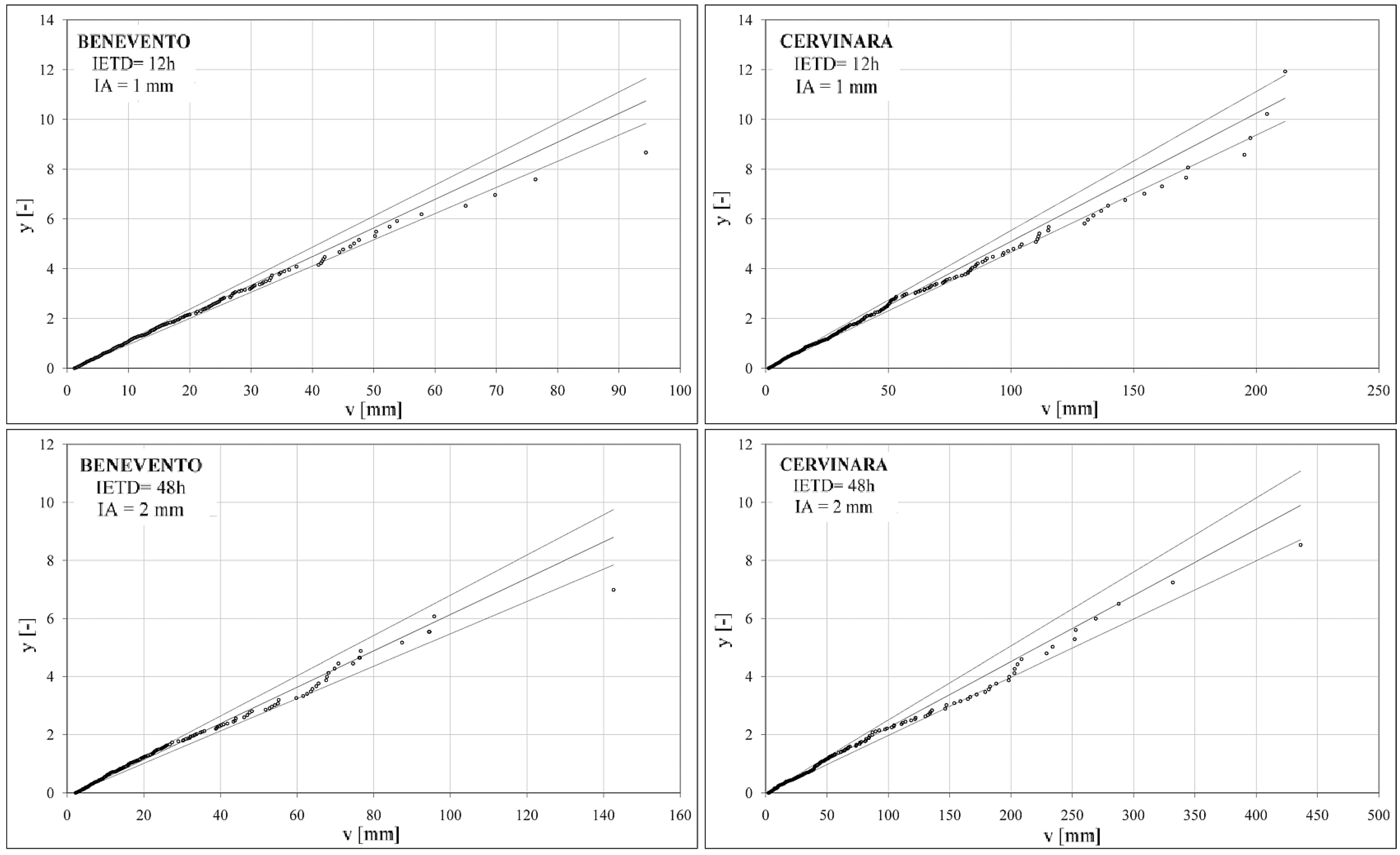
The reliability of the Weibull distribution was verified through the goodness of fit test bond for a significance level α of 0.05.
Figure 6 presents the data and confidence bands for Cervinara and Benevento for values of IETD = 12 h, Ia = 1 mm and IETD = 48 h, Ia = 2 mm. Almost all the sample points fall within the confidence band, so the statistical hypothesis on the applicability of the Weibull distribution for the causal variable v can be considered reliable. For other combinations of IETD and Ia values used with this method, which are not shown for brevity, the hypothesis of applicability is also confirmed.
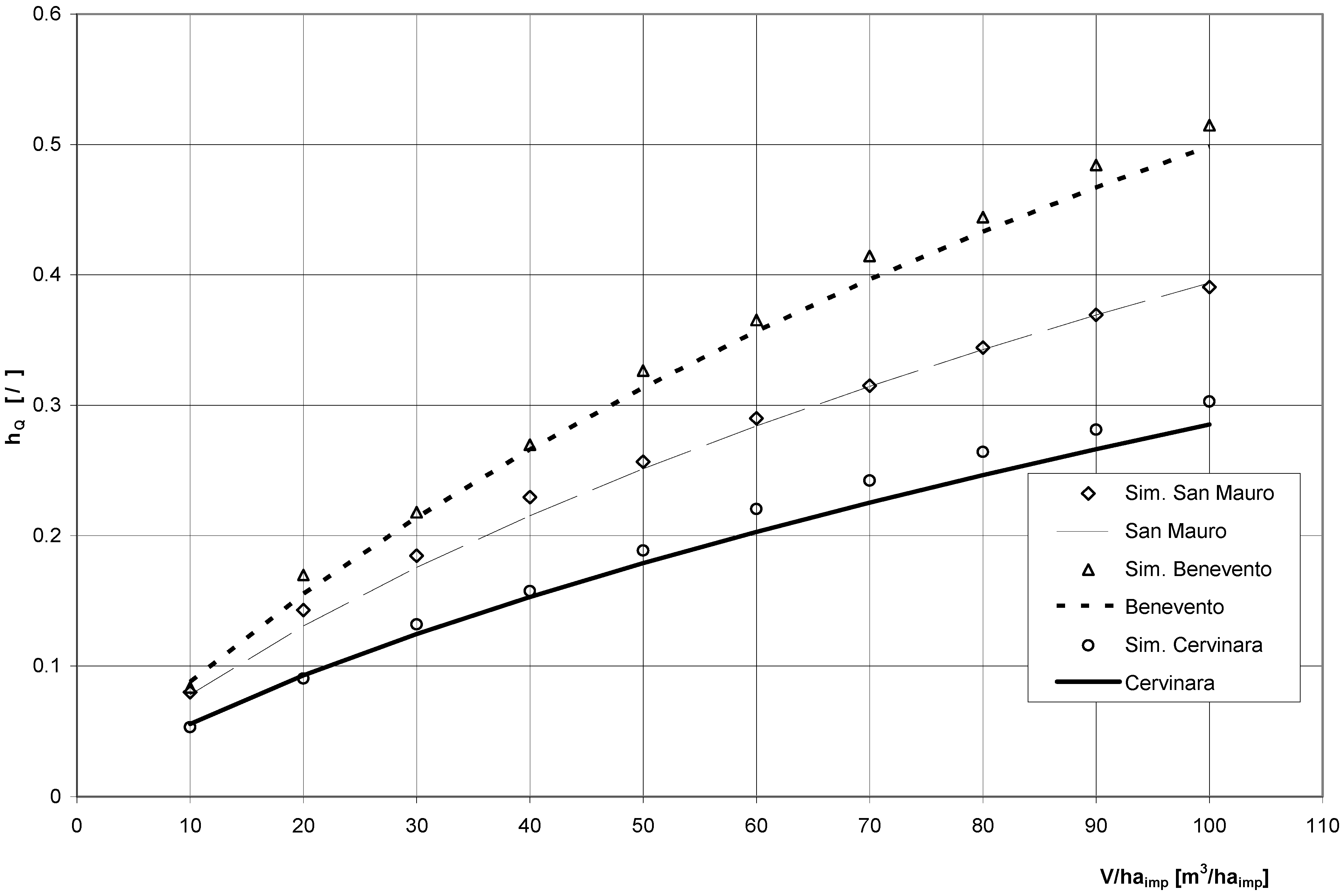
Figure 7 presents the efficiency index trend [
9] at varying tank storage volumes for the three rain station gauges, applying both the continuous simulation approach (points) and semi-probabilistic model (curves).
There is good agreement between the results obtained from the two approaches.
Figure 7 illustrates that for the case under consideration, both approaches are valid for estimating the stormwater tank efficiency in terms of water storage.
Figure 6.
Adaptation of the samples derived from the time series of precipitation of Benevento and Cervinara values for IETD = 12 and 48 h, and Ia = 1 and 2 mm.
Figure 6.
Adaptation of the samples derived from the time series of precipitation of Benevento and Cervinara values for IETD = 12 and 48 h, and Ia = 1 and 2 mm.
Figure 7.
Average annual rainfall events entirely contained by the capture tank (C), varying with the specific volume, obtained using the continuous simulation (points) and semi-probabilistic (curves) values developed for IETD = 48 h and Ia = 1 mm.
Figure 7.
Average annual rainfall events entirely contained by the capture tank (C), varying with the specific volume, obtained using the continuous simulation (points) and semi-probabilistic (curves) values developed for IETD = 48 h and Ia = 1 mm.


