3.1. Average Annual Direct Runoff Computations
To explore the differences in runoff computation approaches, a CN of 85 was selected, which represents cropland with the C hydrologic soil group in the EPA STEPL model. Average annual direct runoff (depth, millimeters) values were computed with the five approaches (
Table 3,
Figure 4). The average annual direct runoff for the first approach (
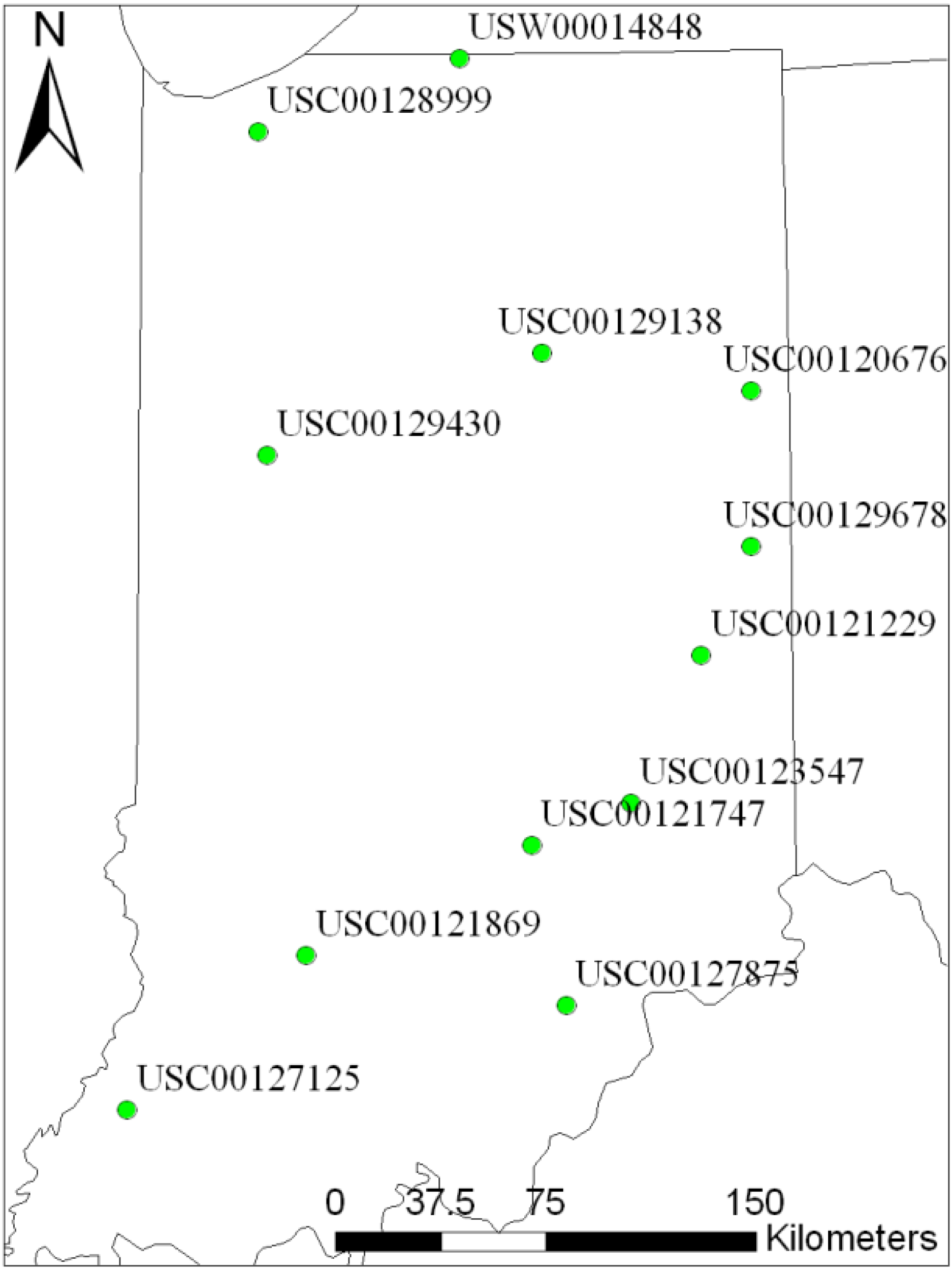
i.e., general use of the SCS-CN method with daily precipitation data, GU) ranged from 117.4 mm (USC00120676) to 191.4 mm (USC00127125). However, the average annual direct runoff estimated by the second approach (
i.e., original EPA STEPL approach, OS) ranged from 242.5 mm (USW00014848) to 339.9 mm (USC00127125). Although identical precipitation data were used for the approaches, the difference between the OS and GU approaches was a minimum of 77.6% (overestimated, USC00127125) and a maximum of 111.8% (overestimated, USC00120676).
Table 3.
Average annual precipitation and direct runoff computations.
Table 3.
Average annual precipitation and direct runoff computations.
| Station | Precipitation (mm) | Average Annual Direct Runoff Depth (mm) | TC8 |
|---|
| PN1 | PC2 | GU3 | CL4 | CS5 | OS6 | ST7 |
|---|
| USC00120676 | 963.8 | 940.7 | 117.4 | 107.4 | 41.6 | 248.6 | 216.0 | 78 |
| USC00121747 | 1077.0 | 1027.1 | 164.9 | 147.9 | 68.0 | 309.4 | 327.8 | 76 |
| USC00121869 | 1128.1 | 1146.3 | 187.7 | 189.3 | 76.1 | 334.4 | 331.8 | 76 |
| USW00014848 | 970.7 | 950.5 | 121.1 | 114.5 | 40.2 | 242.5 | 190.7 | 78 |
| USC00128999 | 1008.6 | 958.9 | 152.6 | 121.4 | 56.0 | 274.4 | 218.4 | 76 |
| USC00129138 | 1025.7 | 925.5 | 143.8 | 120.8 | 54.5 | 280.4 | 215.2 | 77 |
| USC00129430 | 996.0 | 935.1 | 145.3 | 125.1 | 55.6 | 274.8 | 215.2 | 77 |
| USC00129678 | 931.3 | 951.8 | 124.8 | 122.6 | 45.8 | 250.8 | 216.2 | 77 |
| USC00121229 | 1044.5 | 1027.8 | 141.1 | 130.3 | 55.6 | 284.4 | 249.1 | 77 |
| USC00123547 | 994.8 | 1047.9 | 129.6 | 144.1 | 48.4 | 263.9 | 327.8 | 77 |
| USC00127125 | 1080.4 | 1069.2 | 191.4 | 176.4 | 85.6 | 339.9 | 357.0 | 75 |
| USC00127875 | 1097.9 | 1078.6 | 173.0 | 161.6 | 69.6 | 320.8 | 335.7 | 76 |
The third approach (
i.e., corrected EPA STEPL with an initial abstraction coefficient of 0.2, CS) resulted in underestimation compared to the GU for all stations. Moreover, the approach showed no direct runoff when the average rainfall per event for the stations was smaller than 0.2S calculated by CN (Equation (3)), because the average direct runoff depth (Equation (6)) became 0.0 mm, based on Equation (2). Thus, CN needs to be greater than a critical value (TC (curve number threshold to generate direct runoff by CS) in
Table 3) to generate average annual direct runoff greater than 0.0 mm. In other words, there will be no average annual direct runoff in the area with CN values smaller than TC in
Table 3.
Figure 4.
Comparison of average annual direct runoff by different approaches.
Figure 4.
Comparison of average annual direct runoff by different approaches.
Daily precipitation data generated by CLIGEN were used to compute daily direct runoff in the fourth approach (CL). The difference between the CL and GU approaches was a minimum of 0.9% (overestimated, USC00121869) and a maximum of 20.5% (underestimated, USC00128999). In addition, the average annual direct runoff from the CL approach demonstrated smaller differences than the average annual direct runoff by the OS and CS approaches.
The EPA STEPL model was used in the fifth approach (ST, average annual direct runoff by the EPA STEPL model), and the estimated average annual direct runoff ranged from 190.7 mm (USW00014848) to 357.0 mm (USC00127125). The difference between the GU and ST approaches was a minimum of 43.1% (overestimated, USC00128999) and a maximum of 152.9% (overestimated, USC00123547). Similar to the OS approach, the ST results showed large differences relative to the GU results.
The results indicate that average annual direct runoff needs to be the aggregate of daily direct runoff based on daily precipitation data. In other words, the approach to compute average annual direct runoff using the SCS-CN method with average rainfall per event (i.e., the OS and CS approaches) would lead to average annual direct runoff that is much larger than values estimated when the CN runoff method is applied as it was intended. Comparing the OS approach to the CS approach, the OS approach showed large differences at all stations, because the denominators in Equation (6) for the OS approach were smaller than those for the CS approach, since the initial abstraction coefficients were 0.0 for OS and 0.2 for CS. Even though the approach using average rainfall per event was corrected (CS), the approach resulted in underestimation compared to the GU approach. In addition, the CS approach estimated average annual direct runoff greater than 0 mm, only when CN was greater than a critical value (TC), and therefore, there will not be average annual direct runoff in areas with small CNs (e.g., forest). The ST approach resulted in not only overestimation of runoff, but also a large difference compared to runoff from the GU approach. Thus, it was concluded that the approach using the average rainfall per event currently used in the EPA STEPL model is not applicable for computing average annual direct runoff.
The SCS-CN method was developed based on the relationship between rainfall and direct runoff [
11,
18]. SCS-CN is an empirical model composed of two parameters, which are CN and initial abstraction. The initial abstraction was empirically determined to be 0.2 S [
18,
37]. The CN tables published and currently used typically assume that the initial abstraction coefficient is 0.2. The equations in the SCS-CN method need to be modified when other initial abstractions are used [
14,
21]. In addition, the SCS-CN method using an initial abstraction coefficient of 0.2 is typically used to simulate daily-based direct runoff using daily rainfall in hydrologic models [
12,
13,
14,
15,
16].
Since the SCS-CN method is an empirical model, its assumptions must be maintained if it is to provide accurate runoff estimates. Therefore, the initial abstraction needs to be 0.2 S for the CN values commonly used; otherwise, CNs need to be adjusted for other initial abstraction values. The method must also be used for event- or daily-based direct runoff with event- or daily-based rainfall. In other words, average annual direct runoff needs to be computed by aggregating daily direct runoff obtained using daily rainfall. If the assumptions are not maintained in the use of the SCS-CN method, large differences in the results compared to those for the general use of the SCS-CN method may result. For instance, the OS approach used a different initial abstraction (i.e., 0.0S) and did not adjust CNs, and thus, the approach resulted in overestimation compared to the GU approach. When the initial abstraction coefficient was corrected (CS), average annual direct runoff resulted in underestimation compared to the GU approach, because the CS approach used a single rainfall value (average rainfall per event) for average annual direct runoff estimation.
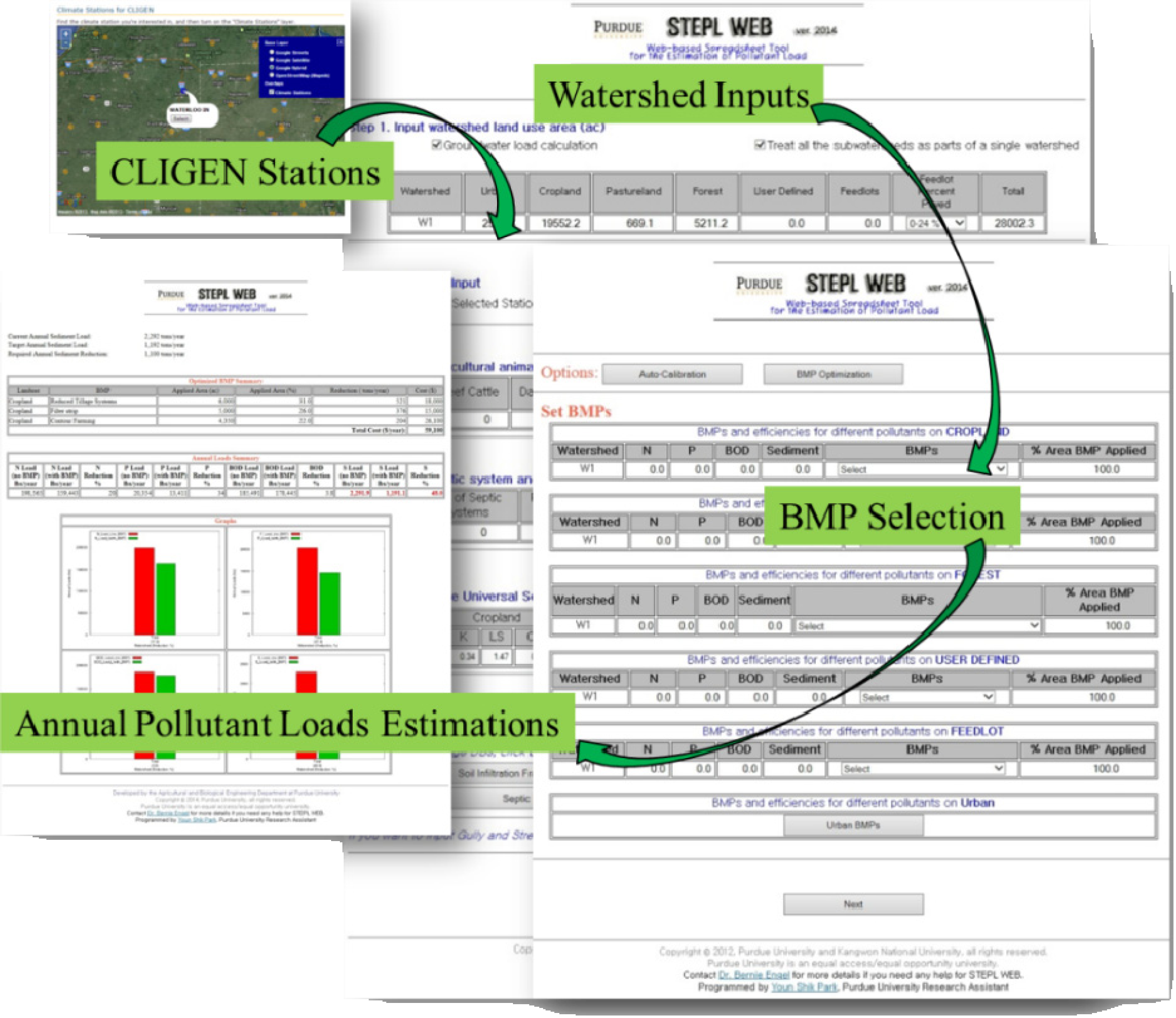
3.2. Application of STEPL WEB
To demonstrate the BMP simulation ability of STEPL WEB, a watershed named the Tippecanoe River at North Webster in northeastern Indiana (
Figure 5) was selected. The spatial input datasets to delineate the watershed and to prepare STEPL WEB inputs were the 30-meter resolution digital elevation model (DEM) from the United States Geological Survey (USGS) National Elevation Dataset, the National Land Cover Dataset, 2006 (NLCD 2006), from the USGS, and the Soil Survey Geographic Database (SSURGO) from the United States Department of Agriculture (USDA). The watershed area is 129.1 km
2, with 61.3% of the watershed land use being cropland (
Figure 5,
Table 4).
The Web-based LDC Tool was used to collect flow data from the USGS station number 03330241 (Tippecanoe River at North Webster, IN, USA). Total phosphorus data were collected from the Indiana Department of Environmental Management (IDEM) at the same location. The period selected to develop a load duration curve was from 25 March 1998 to 17 November 2010, based on the water quality data period. The standard concentration for total phosphorus was set to 0.08 mg/L [
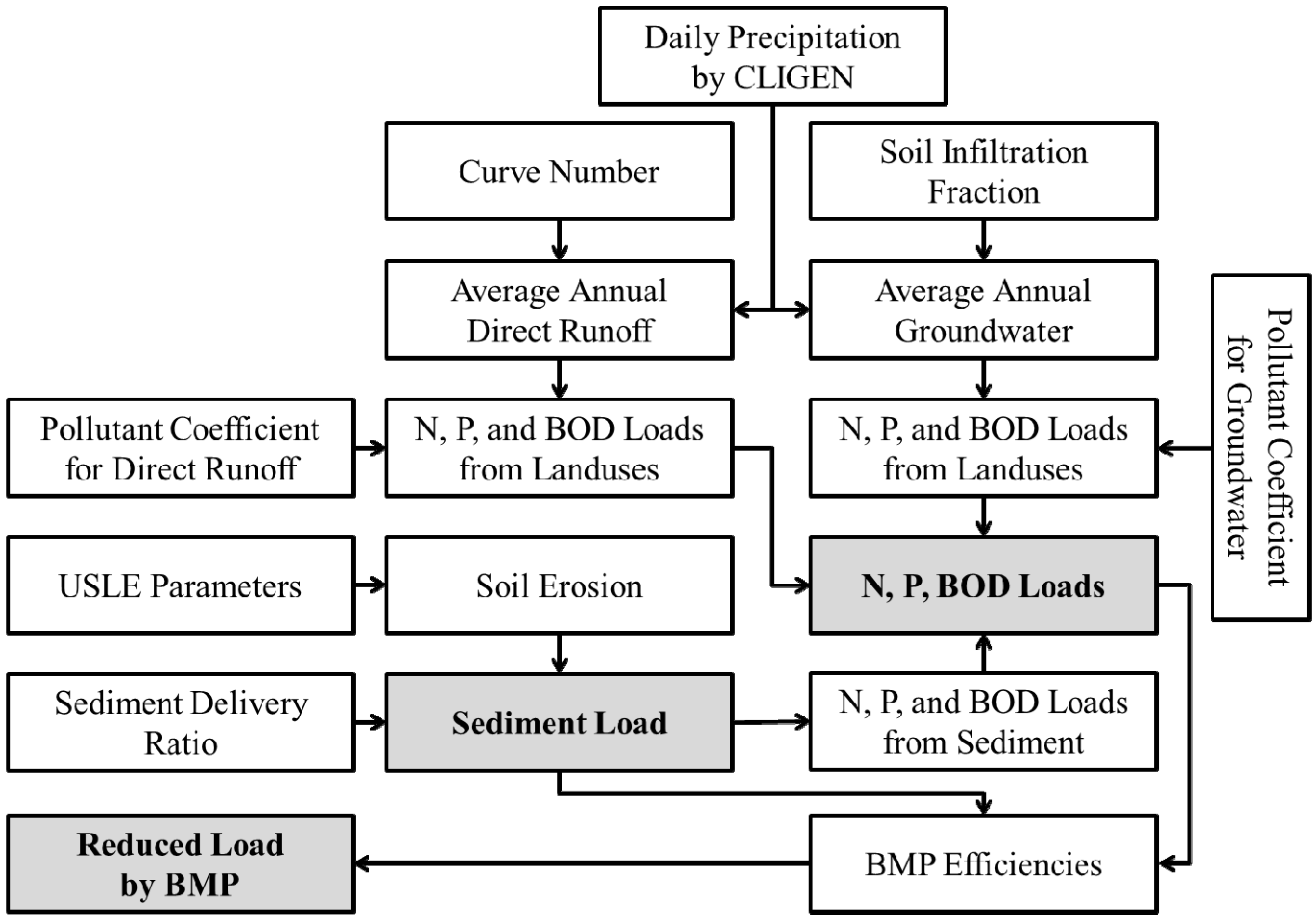
38]. Average annual direct runoff, average annual baseflow and average annual sediment load were computed with the Web-based LDC Tool. Nutrient loads in STEPL WEB are computed based on loads from runoff, as well as sediment, and therefore, the average annual sediment load is required to calibrate model parameters for average annual nutrient loads. LOADEST [
39] was used for average annual sediment load calculation. The model parameters in STEPL WEB were calibrated (
Table 5 and
Table 6) using the auto-calibration module using the bisection method. The Web-based LDC Tool identified the required phosphorus pollutant reduction percentage to be 11% to meet the standard load. STEPL WEB then established cost-effective BMP lists based on least cost per unit of pollutant reduction. The most cost-effective BMP was filter strip for cropland; reduced tillage systems and contour farming were the second and third most cost-effective BMPs. The fourth and fifth most cost-effective BMPs were vegetated filter strips and bioretention facility for urban.
Figure 5.
Land uses of the Tippecanoe River at North Webster watershed. USGS, United States Geological Survey.
Figure 5.
Land uses of the Tippecanoe River at North Webster watershed. USGS, United States Geological Survey.
Table 4.
Land use distribution for the study watershed.
Table 4.
Land use distribution for the study watershed.
| Land use | Area (km2) | Percentage (%) |
|---|
| Urban | 10.4 | 8.1 |
| Cropland | 79.2 | 61.3 |
| Pasture | 2.7 | 2.1 |
| Forest | 21.1 | 16.3 |
| Water | 15.7 | 12.2 |
| Total | 129.1 | 100.0 |
Two scenarios for BMP application in the watershed were simulated. One was the application of filter strip on up to 79 km2 (100% of the cropland area). The other was the application of filter strip on up to 10 km2 in the cropland area and reduced tillage systems on up to 10 km2 of cropland; contour farming was considered not applicable, and vegetative filter strips were possible on up to 5 km2 in urban area. In the first scenario, filter strip for cropland needed to be applied to 17 km2 of cropland to reach the pollutant reduction goal, with an estimated annual cost of $12,870. In the second scenario, filter strip needed to be applied to 10 km2 of cropland; reduced tillage systems needed to be applied to 10 km2 of cropland, and vegetative filter strips needed to be applied to 4 km2 of urban as the optimal solution. The estimated annual cost was $17,400, which resulted from $7,650 for filter strip, which provided 147.5 kg/year phosphorus reduction in cropland, $7,710 for reduced tillage systems with 95.6 kg/year phosphorus reduction in cropland and $2,040 for vegetative filter strips with 1.0 kg/year phosphorus reduction in urban. Both scenarios met the required reduction; however, the estimated annual cost of the second scenario was more expensive than the first scenario, but the first scenario may not be feasible if ‘filter strip’ application is not possible to implement on 17 km2 or more of cropland area.
Table 5.
STEPL WEB parameters (default/calibrated).
Table 5.
STEPL WEB parameters (default/calibrated).
| Model Parameters | HSG | A | B | C | D |
|---|
| Curve Number | Urban | 83/90 | 89/97 | 92/98 | 93/98 |
| Cropland | 67/73 | 78/85 | 85/92 | 89/97 |
| Pastureland | 49/53 | 69/75 | 79/86 | 84/91 |
| Forest | 39/42 | 60/65 | 73/79 | 79/86 |
| Soil Infiltration Fraction | Urban | 0.36/0.31 | 0.24/0.21 | 0.12/0.01 | 0.06/0.05 |
| Cropland | 0.45/0.39 | 0.30/0.26 | 0.15/0.13 | 0.08/0.07 |
| Pastureland | 0.45/0.39 | 0.30/0.26 | 0.15/0.13 | 0.08/0.07 |
| Forest | 0.45/0.39 | 0.30/0.26 | 0.15/0.13 | 0.08/0.07 |
| Pollutant Coefficient Phosphorus (mg/L) | Urban | 0.30/0.18 |
| Cropland | 0.50/0.30 |
| Pastureland | 0.30/0.18 |
| Forest | 0.10/0.06 |
| Sediment Delivery Ratio | 0.42 × (0.3861 × Area (km2))−0.1350/0.02 × (0.3861 × Area (km2))−0.1350 |
Table 6.
Average annual direct runoff, baseflow and sediment load.
Table 6.
Average annual direct runoff, baseflow and sediment load.
| Model Outputs | Measured | Predicted |
|---|
| Direct Runoff | 16.7 × 10⁶ m3/year | 16.7 × 10⁶ m3/year |
| Baseflow | 25.9 × 10⁶ m3/year | 25.6 × 10⁶ m3/year |
| Sediment | 237 ton/year | 245 ton/year |
| Phosphorus | 2.3 ton/year | 2.3 ton/year |


