3.1. Assessing Acceptable Estimated Parameter Sets
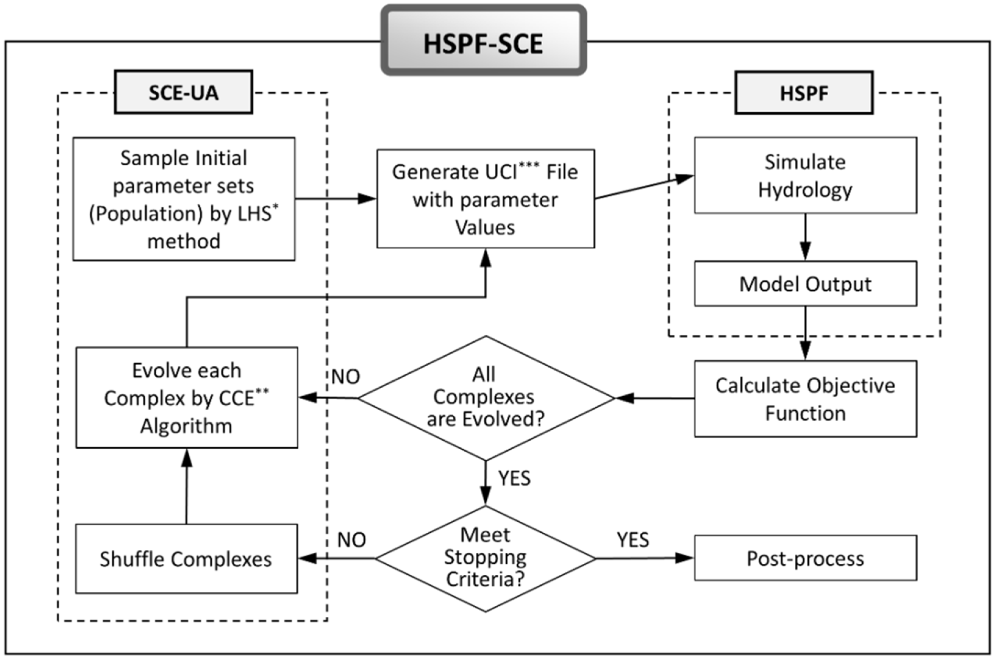
In this study, three HSPF hydrologic models were calibrated using the HSPF-SCE auto calibration tool. The HSPF-SCE tool was allowed to calibrate nine parameters, with one of those allowed to vary seasonally for a total of ten calibration parameters. In the calibration processes, the SCE-UA algorithm identified multiple parameter sets that satisfied the six HSPEXP model performance criteria while minimizing objective function values. For example, for the Reed Creek watershed, 252 parameter sets out of 504 possible parameter sets were found to meet all the six HSPXEP criteria.
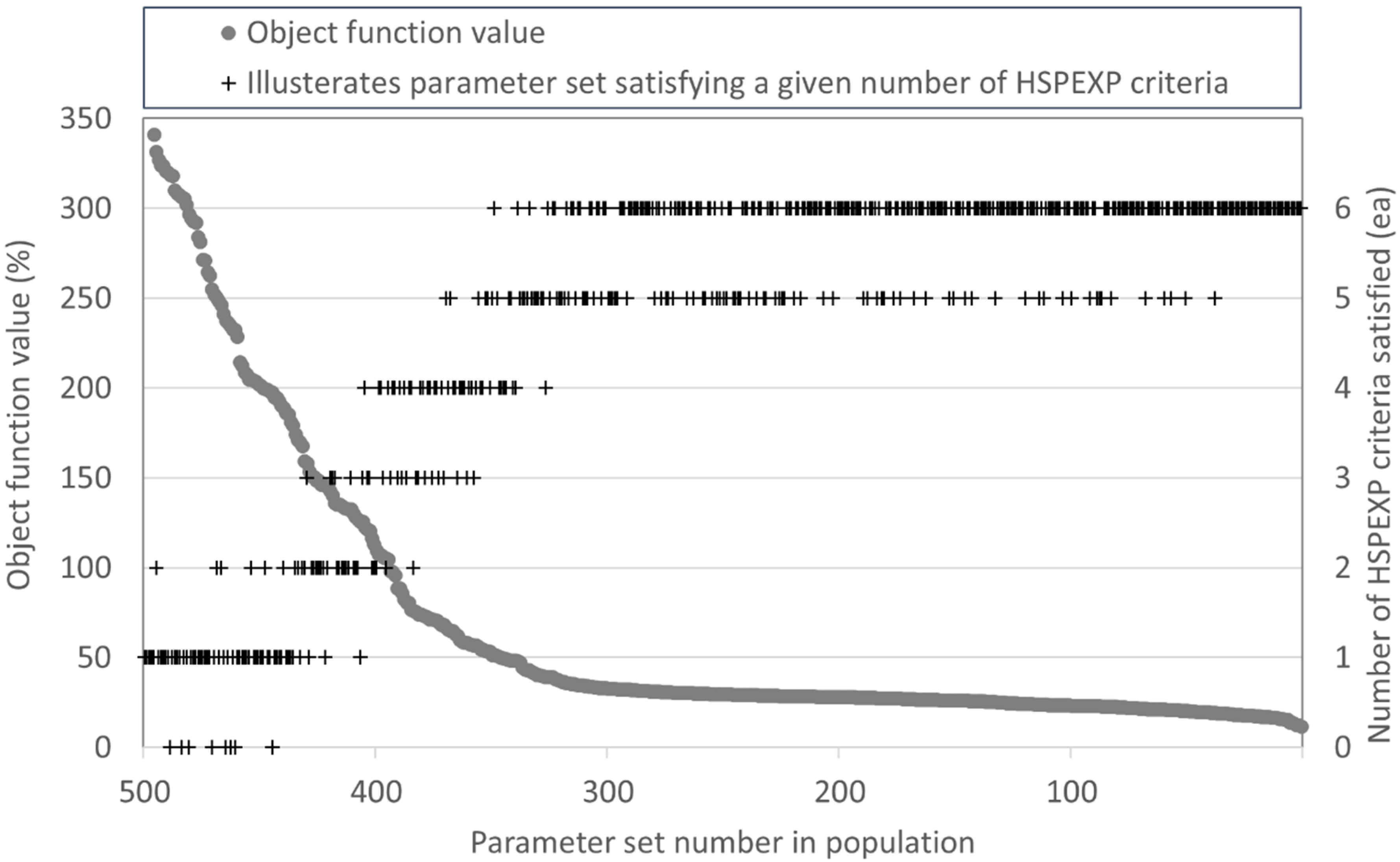
Figure 3 shows the Reed Creek distribution of the objective function values on the left y-axis and the number of HSPEXP criteria satisfied by the parameter sets in the last iteration of the optimization process on the right y-axis. Parameter sets began meeting all six HSPEXP criteria once the value of the objective function decreased to approximately 50%. The minimum objective function value was 11.6%. For the Piney River and Pigg River watersheds, 159 and 141 parameter sets satisfied all six HSPEXP criteria, respectively. The parameter sets that met all six HSPEXP calibration criteria are referred to herein as “qualified” parameter sets.
Figure 3.
Objective function values and the number of HSPEXP criteria met by the final parameter set population using the SCE-UA algorithm of HSPF-SCE (Reed Creek watershed).
Figure 3.
Objective function values and the number of HSPEXP criteria met by the final parameter set population using the SCE-UA algorithm of HSPF-SCE (Reed Creek watershed).
Performance statistics produced by the qualified parameter sets are shown in
Figure 4. For the Reed Creek watershed, hydrologic simulation using the 252 qualified parameter sets produced statistics in the “very good” ranges for monthly PBIAS, monthly NSE, and monthly RSR with some “good” measures for monthly R
2 (
Table 4). The 159 qualified parameter sets for the Piney River watershed were in the ranges of between “good” and “fair” for monthly NSE and monthly RSR, “very good” for monthly PBIAS, but monthly R
2 values were in between “fair” and “poor”. On the other hand, the 141 qualified parameter for the Pigg River watershed yielded relatively unsatisfactory performance statistics, and values of monthly NSE, monthly RSR, monthly R
2 and daily R
2 were classified as “poor”. Karst topography including sink holes and springs that frequently appear in the Ridge and Valley physiographic region of Virginia [
61] could be one possible reason for the poor model performance in the Pigg River watershed. HSPF has limited groundwater simulation capabilities, and representing karst hydrology using HSPF is challenging.
Once multiple parameter sets that met all the HSPEXP criteria were identified, a single parameter set expected to best represent the hydrologic processes of a study watershed was selected from the pool of qualified parameter sets. This selection was based on model performance statistics, visual comparisons of various model output graphics (e.g.,
Figure 5), and best professional judgment. For example, for the Reed Creek watershed, 160 parameter sets out of 252 were qualified, meaning they satisfied all six HSPEXP criteria for both the calibration and validation period. The 160 qualified parameter sets were then classified into groups based on five performance statistics as shown in
Table 5 and
Table 6. Parameter sets belonging to the same group were regarded as equal in terms of model performance. In addition to the comparison of performance statistics presented in
Table 5 and
Table 6, the qualified parameter sets classified into Group 1 were further assessed by visually comparing hydrographs and flow duration curve plots simulated using those Group 1 parameter sets.
Figure 4.
Qualified parameter set model performance plots. Data generated by running HSPF with each qualified parameter set, then comparing observed and simulated model output using four model performance measures (a) Monthly PBIAS and Monthly NSE; and (b) Monthly R2 and Monthly RSR. The square, triangle, and diamond correspond to the parameter set selected by the authors for subsequent HSPF simulations and model performance evaluation.
Figure 5.
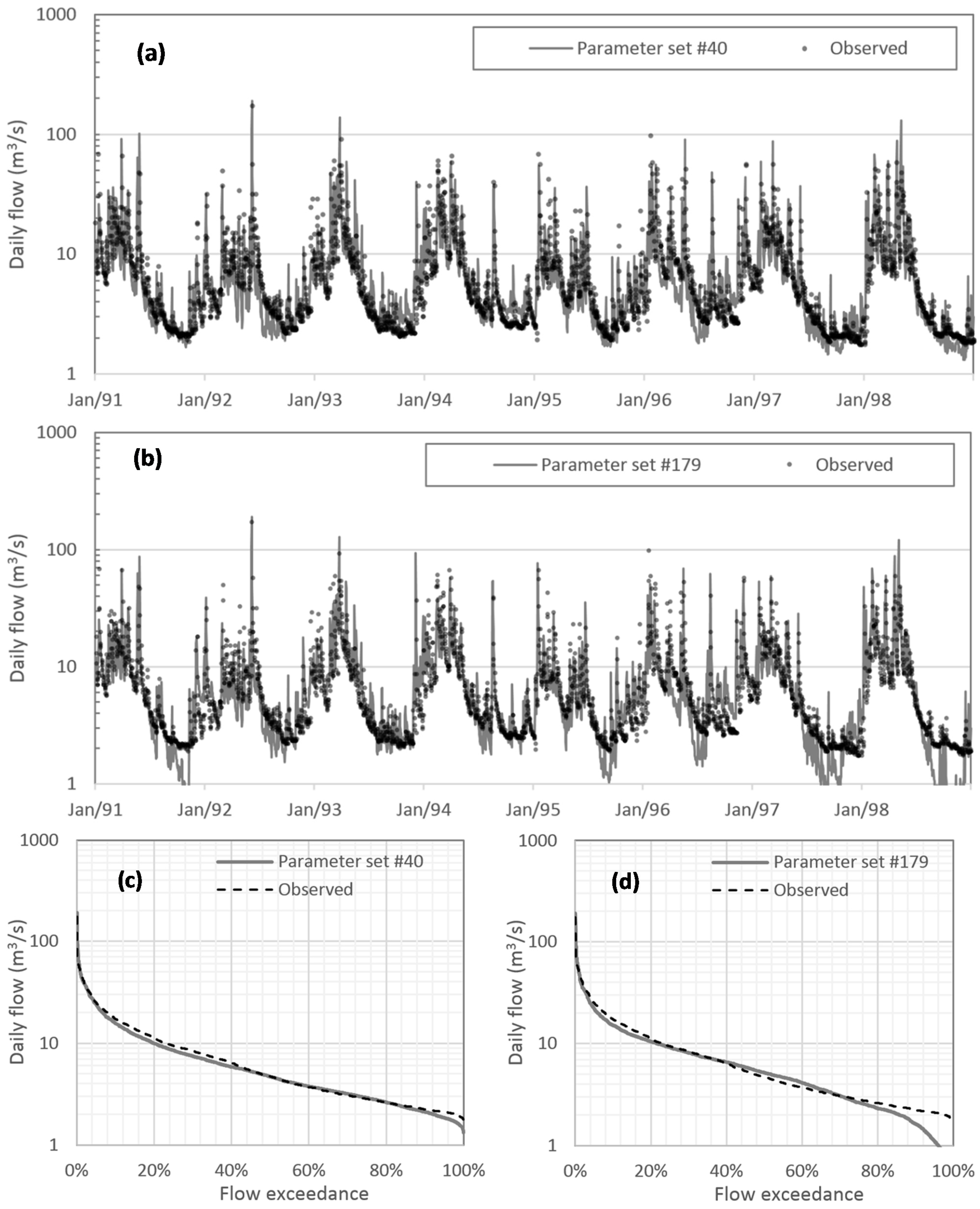
Comparison of the observed and simulated daily hydrographs with parameter set No. 40 (a,c) and No. 179 (b,d) for the Reed Creek watershed; (a,b) are daily log-scale hydrographs; and (c,d) are flow duration curves of daily flow.
Figure 5.
Comparison of the observed and simulated daily hydrographs with parameter set No. 40 (a,c) and No. 179 (b,d) for the Reed Creek watershed; (a,b) are daily log-scale hydrographs; and (c,d) are flow duration curves of daily flow.
Table 5.
Classification of the parameter sets identified by HSPF-SCE in terms of model performance statistics (for the Reed Creek watershed).
Table 5.
Classification of the parameter sets identified by HSPF-SCE in terms of model performance statistics (for the Reed Creek watershed).
| Group | Parameter Set ID | Daily R2 | Monthly R2 | Monthly RSR | Monthly PBIAS | Monthly NSE |
|---|
| Group 1 | 35 | 0.608 | Fair | 0.873 | Very good | 0.408 | Very good | −4.130 | Very good | 0.834 | Very good |
| 40 * | 0.632 | 0.908 | 0.435 | −6.626 | 0.811 |
| 95 | 0.605 | 0.866 | 0.401 | −4.857 | 0.839 |
| 98 | 0.601 | 0.862 | 0.444 | −6.180 | 0.803 |
| 142 | 0.606 | 0.870 | 0.361 | −3.277 | 0.870 |
| 171 | 0.626 | 0.886 | 0.477 | −4.539 | 0.772 |
| 179 | 0.610 | 0.864 | 0.345 | −3.826 | 0.881 |
| 196 | 0.615 | 0.872 | 0.414 | −5.071 | 0.828 |
| 256 | 0.611 | 0.869 | 0.432 | −4.841 | 0.814 |
| 278 | 0.609 | 0.866 | 0.386 | −4.393 | 0.851 |
| Group 2 | 192 | 0.622 | Fair | 0.885 | Very good | 0.512 | Good | −6.954 | Very good | 0.737 | Good |
| 221 | 0.603 | 0.871 | 0.534 | −7.817 | 0.715 |
| 242 | 0.605 | 0.872 | 0.502 | −3.543 | 0.748 |
| Group 3 | 157 | 0.601 | Fair | 0.841 | Good | 0.549 | Good | −5.498 | Very good | 0.699 | Good |
| Group 4 | 216 | 0.593 | Poor | 0.868 | Very good | 0.484 | Very good | −7.103 | Very good | 0.765 | Very good |
| 204 | 0.592 | 0.879 | 0.474 | −4.970 | 0.776 |
| 212 | 0.598 | 0.870 | 0.450 | −5.845 | 0.798 |
Table 6.
The HSPEXP criteria values of Groups 1 to 4 (for the Reed Creek watershed).
Table 6.
The HSPEXP criteria values of Groups 1 to 4 (for the Reed Creek watershed).
| Group | Parameter set ID | Total Volume (±10%) | 50% Lowest Flows (±10%) | 10% Highest Flows (±15%) | Storm Peaks (±15%) | Seasonal Volume (±10%) | Seasonal Storm Volume (±15%) |
|---|
| Group 1 | 35 | −4.77 | −6.15 | −2.83 | 2.13 | 1.44 | −1.60 |
| 40 * | −4.68 | −0.52 | −0.70 | 6.60 | 6.66 | −0.26 |
| 95 | −3.97 | −7.24 | −1.41 | 5.90 | 3.49 | −1.26 |
| 98 | −5.40 | −3.49 | −4.64 | 0.84 | 5.68 | −3.23 |
| 142 | −6.32 | −5.45 | −2.91 | 5.17 | 3.64 | −2.44 |
| 171 | −4.07 | −9.80 | −1.90 | 2.47 | 8.08 | −0.72 |
| 179 | −4.99 | −5.09 | −5.80 | 1.49 | 5.30 | −4.55 |
| 196 | −4.38 | −5.77 | −2.76 | 3.63 | 9.44 | −2.02 |
| 256 | −6.61 | −9.81 | −5.09 | 3.23 | 0.85 | −4.23 |
| 278 | −5.62 | −9.65 | −3.33 | 3.47 | 6.48 | −2.73 |
| Group 2 | 192 | −3.93 | −6.52 | −4.83 | 3.75 | 4.17 | −4.69 |
| 221 | −4.94 | −1.88 | −2.69 | 6.03 | 9.71 | −3.30 |
| 242 | −5.65 | −2.48 | −4.89 | 4.17 | 7.47 | −4.67 |
| Group 3 | 157 | −2.27 | −8.62 | 1.46 | 7.00 | −3.53 | 3.50 |
| Group 4 | 216 | −5.53 | 1.83 | 0.66 | 9.43 | 9.78 | −1.21 |
| 204 | −3.92 | −2.08 | 2.83 | 8.84 | 8.61 | 1.87 |
| 212 | −5.63 | −8.08 | 0.53 | 9.59 | 4.45 | −0.12 |
To illustrate the graphical/visual model performance evaluation, the daily flow time-series and flow duration curve simulated using two of the qualified parameter sets (
i.e., No. 40 and No. 179 in
Table 5 and
Table 6) are plotted in
Figure 5. Although parameter set No. 179 provided better monthly RSR, PBIAS, and NSE than did No. 40 (
Table 5), the graphical comparison (
Figure 5) clearly shows parameter set No. 40 yielded a better match to the observed flow. Thus, parameter set No. 40 was selected as the final parameter set to simulate the hydrology for the Reed Creek watershed. The same parameter selection process was applied to the Pigg and Piney River watersheds.
3.2. Comparing Automated and Manual Calibration Parameter Sets
Manually calibrated parameter values were compared with the selected qualified parameter set identified by HSPF-SCE.
Table 7 presents the comparison for all three watersheds, while
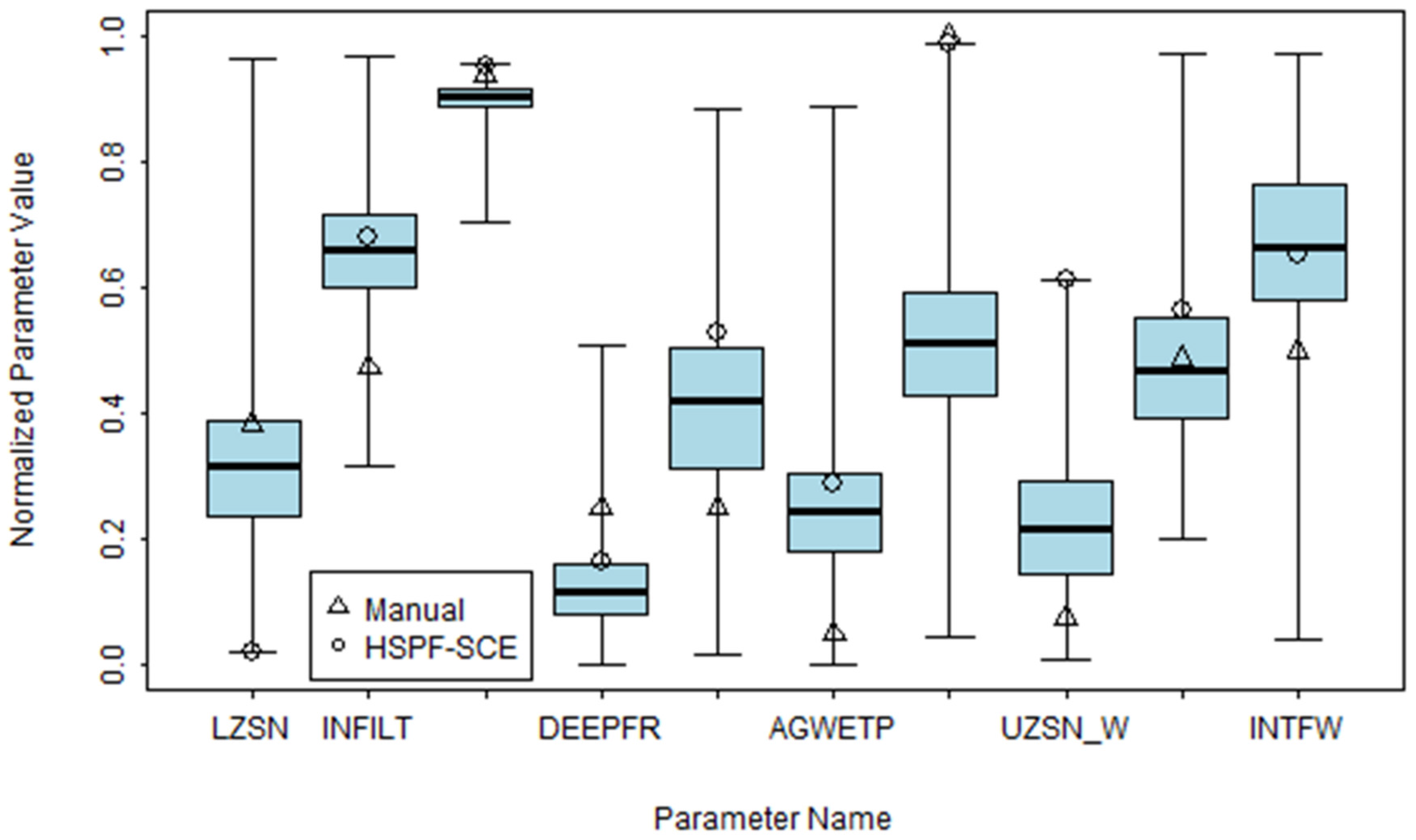
Figure 6 illustrates those comparisons graphically for the Reed Creek watershed. The manual and automated approaches provided quite different ranges for some parameters: LZSN, UZSN, INFILT, BASETP, and AGWETP.
Figure 6 shows box plots for the automated calibrated parameters for the Reed Creek model qualified parameter sets. In
Figure 6, the interquartile ranges (IQR) of selected parameters (INFILT, AGWRC, DEEPFR, BASETP, AGWETP, IRC, INTFW, and UZSN–winter season) do not include the manually calibrated values implying that manual calibration is likely to fall in a local optimum in the parameter space. This finding does not agree with Kim
et al. [
5], who found general agreement among manually calibrated and PEST calibrated parameter values. The discrepancy between this study and Kim
et al. [
5] might be due to the use of different automated optimization algorithms (SCE-UA
vs. PEST) and subjectivity in selecting a final parameter set from the pool of qualified parameter sets.
Table 7.
Comparison of parameter values calibrated by HSPF-SCE and manually.
Table 7.
Comparison of parameter values calibrated by HSPF-SCE and manually.
| Parameter | Piney River Watershed | Pigg River Watershed | Reed Creek Watershed |
|---|
| HSPF-SCE | Manual | HSPF-SCE | Manual | HSPF-SCE | Manual |
|---|
| LZSN | 170.993 | 165.100 | 261.493 | 228.600 | 58.115 | 177.800 |
| UZSN | 31.496 *, 26.416 ** | 24.130–34.290 | 20.828 *, 27.940 ** | 8.890–25.400 | 31.750 *, 29.210 ** | 5.080 *, 25.400 ** |
| INFILT | 0.432–3.810 | 0.229–1.981 | 1.524–3.912 | 2.438–6.223 | 0.711–4.902 | 0.508–3.505 |
| BASETP | 0.072 | 0.000 | 0.091 | 0.150 | 0.106 | 0.050–0.060 |
| AGWETP | 0.007 | 0.000 | 0.022 | 0.100 | 0.058 | 0.010 |
| INTFW | 1.999 | 3.000 | 1.621 | 1.000 | 2.305 | 2.000 |
| IRC | 0.598 | 0.810 | 0.544 | 0.300 | 0.698 | 0.700 |
| AGWRC | 0.959 | 0.960, 0.965 | 0.994 | 0.990 | 0.992 | 0.990 |
| DEEPFR | 0.008 | 0.010 | 0.165 | 0.100 | 0.033 | 0.050 |
Figure 6.
Comparison of parameter values calibrated by the HSPF-SCE and manually calibrated parameter values for the Reed Creek watershed (UZSN_W is for winter season and UZSN_N is for non-winter season).
Figure 6.
Comparison of parameter values calibrated by the HSPF-SCE and manually calibrated parameter values for the Reed Creek watershed (UZSN_W is for winter season and UZSN_N is for non-winter season).
3.3. Comparison of Model Performance between Automatic and Manual Calibration
Hydrographs simulated with the selected qualified parameter sets were evaluated in terms of the six HSPEXP criteria. As seen in
Table 8, both manually and HSPF-SCE calibrated parameters produced model output that meet all the criteria. The HSPF-SCE calibrated parameter set consistently provided lower bias in simulation of total volume compared to the manually calibrated parameters. Goodness-of-fit measures for the selected parameter sets are presented in
Table 9. In general, the selected parameter values calibrated using HSPF-SCE provided performance statistics better than or equivalent to those calibrated manually. The measures of the Piney River watershed indicated “fair” to “very good” in the calibration period and “good” to “very good” in the validation period for both calibration methods. For the Reed Creek watershed, relatively great differences were found in the performance statistics compared to the other watersheds. HSPF-SCE provided statistics in the “very good” range, while those of the manual method were in “fair” to “good” in the both the calibration and validation periods. The selected parameter set for the Pigg River watershed gave “unsatisfactory” modeling results in terms of R
2, RSR and NSE in the calibration period. In all the cases, PBIAS values fell in the “very good” range.
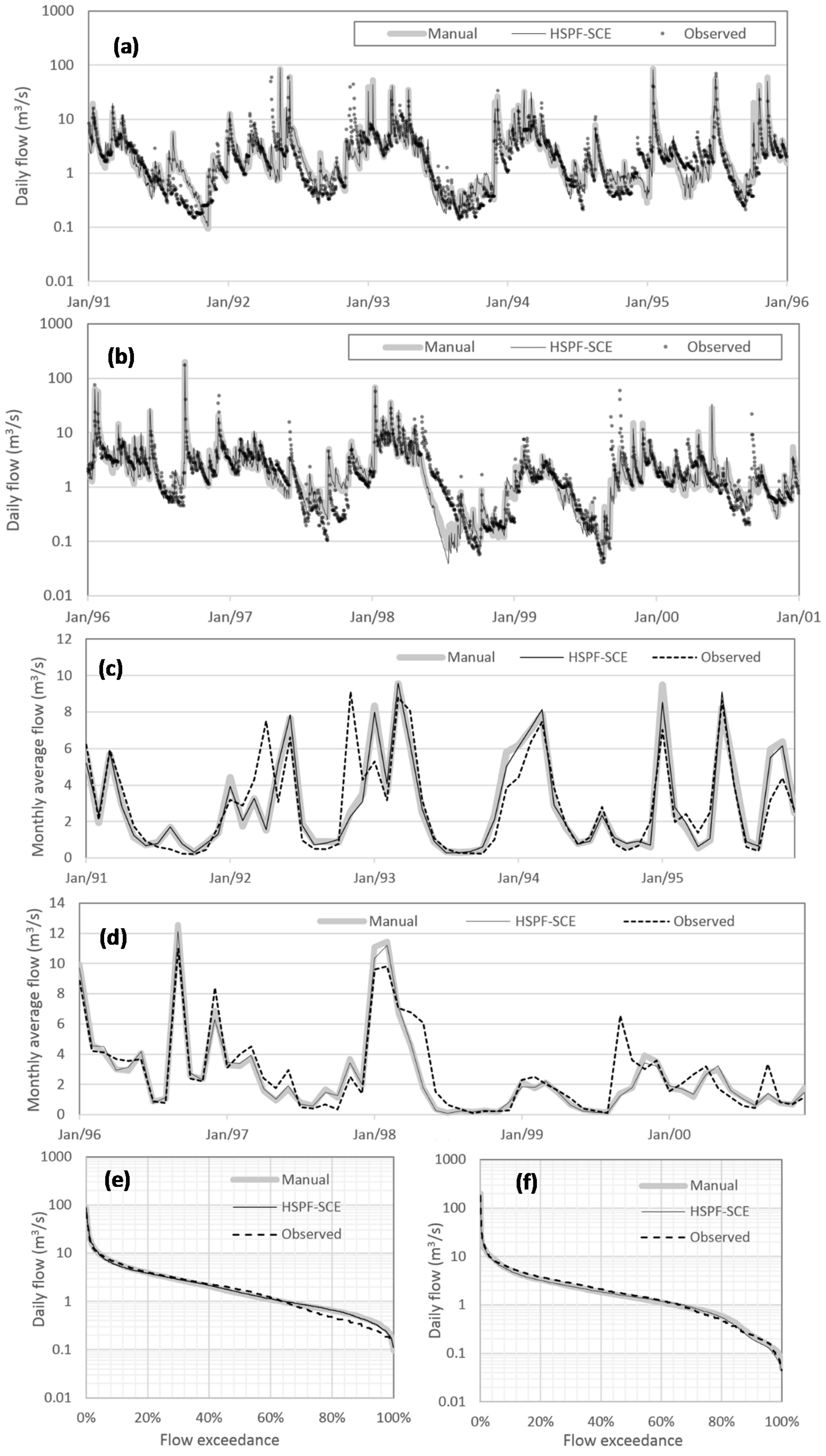
Piney River observed and simulated daily and monthly flow and flow exceedance curves are compared in
Figure 7,
Figure 8 and
Figure 9. Overall, flows simulated using the HSPF-SCE calibrated parameters are similar to those simulated using the manual calibration method, especially for baseflow and high peaks (
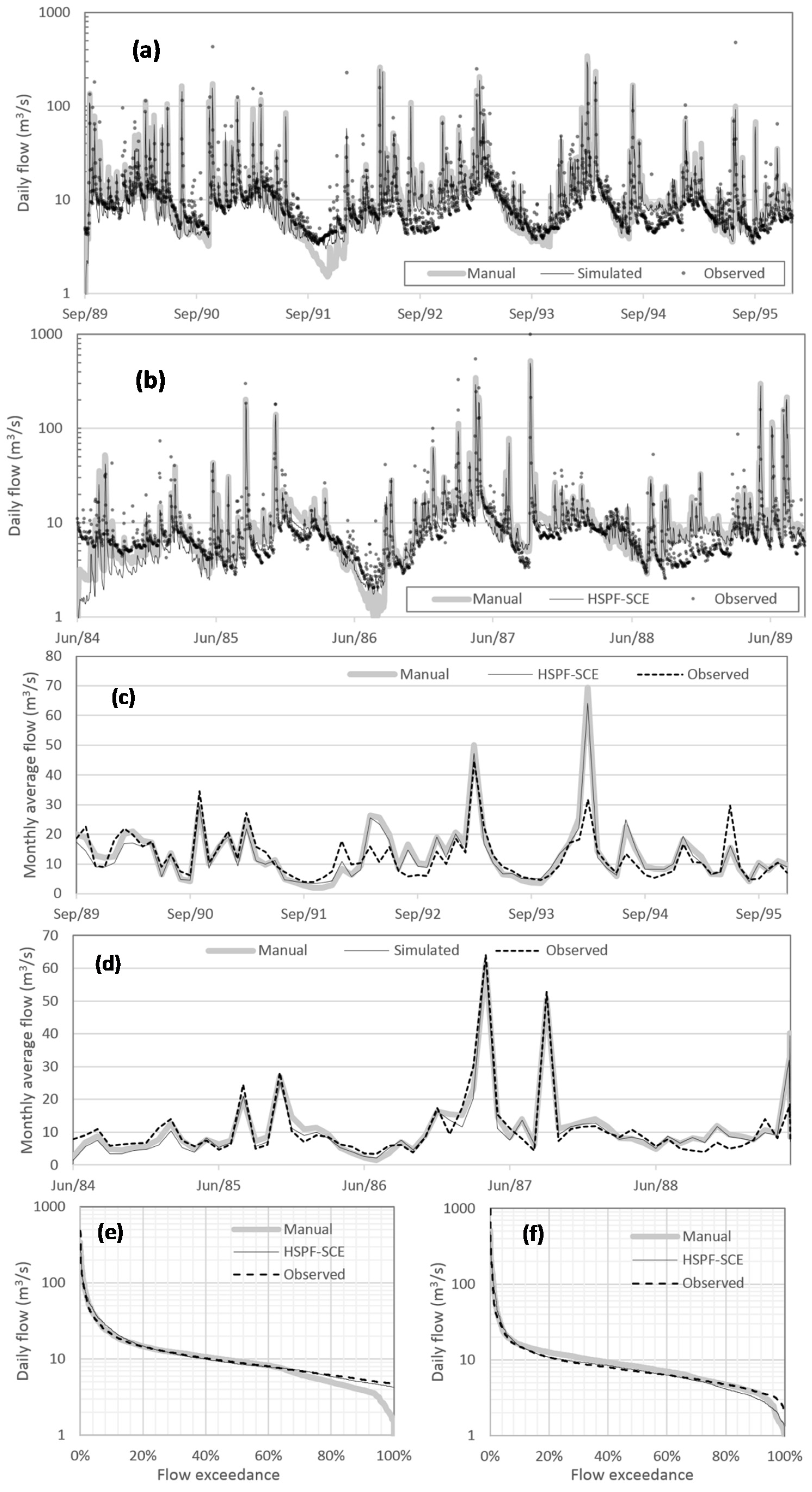
Figure 7). In the Pigg River watershed, overestimation and underestimation of stream flow are found in 1992 of the calibration period and the first year of the validation period, respectively. The HSPF-SCE calibrated parameter values resulted in better simulation results under the low-flow conditions of 1986 and 1991 than the manually calibrated parameters. In general, the HSPF-SCE calibrated parameters provided better agreement with the observed flow than did the manually calibrated parameters (
Figure 8). In the Reed Creek watershed, the simulated and observed flow hydrographs showed better agreement in the calibration period than the validation period (
Figure 9). The relative difference of the model performance for the calibration and validation periods is reflected in the statistics presented in
Table 9.
Table 8.
Comparison of model performance achieved by the calibrated parameters in terms of the six HSPEXP criteria.
Table 8.
Comparison of model performance achieved by the calibrated parameters in terms of the six HSPEXP criteria.
| Watershed | Calibration Method | Periods | Total Volume (±10%) | 50% Lowest Flows (±10%) | 10% Highest Flows (±15%) | Storm Peaks (±15%) | Seasonal Volume (±10%) | Seasonal Storm Volume (±15%) |
|---|
| Piney River | HSPF-SCE | Calibration | −0.3 | 6.9 | 4.0 | 2.6 | 1.1 | 13.2 |
| Validation | −8.5 | −0.5 | −6.2 | −7.0 | −8.6 | 14. 8 |
| Manual | Calibration | 0.7 | 5.9 | 5.9 | 6.5 | −0.5 | 10.5 |
| Validation | −7.8 | −0.5 | −5.3 | −5.8 | −9.2 | 12.2 |
| Pigg River | HSPF-SCE | Calibration | 2.4 | −4.3 | 9.0 | −2.7 | 3.7 | 14.6 |
| Validation | 0.9 | −7.3 | 3.9 | −13.5 | 9.0 | 2.6 |
| Manual | Calibration | 7.8 | −3.3 | 13.2 | −0.3 | 1.5 | 14.4 |
| Validation | 7.1 | 2.6 | 2.4 | −10.4 | 2.8 | −2.0 |
| Reed Creek | HSPF-SCE | Calibration | −4.7 | −0.5 | −0.7 | 6.6 | 6.7 | 13.7 |
| Validation | −6.8 | 1.1 | −1.8 | −14.3 | −1.0 | −6.4 |
| Manual | Calibration | −5.9 | 8.2 | −4.0 | 6.5 | 5.0 | 12.4 |
| Validation | −6.8 | 3.9 | −3.5 | −6.9 | 6.9 | −6.8 |
Table 9.
Comparison of the model performance achieved by the calibrated parameters in terms of common goodness-of-fit measures.
Table 9.
Comparison of the model performance achieved by the calibrated parameters in terms of common goodness-of-fit measures.
| Watershed | Calibration Method | Temporal Scale | Calibration | Validation |
|---|
| R2 | RSR | PBIAS | NSE | R2 | RSR | PBIAS | NSE |
|---|
| Piney River | HSPF-SCE | Daily | 0.66 | 0.97 | −0.29 | 0.05 | 0.79 | 0.47 | −8.52 | 0.78 |
| Monthly | 0.69 | 0.59 | −0.37 | 0.66 | 0.82 | 0.44 | −8.50 | 0.81 |
| Manual | Daily | 0.29 | 1.02 | 0.58 | −0.03 | 0.79 | 0.48 | −7.81 | 0.77 |
| Monthly | 0.68 | 0.60 | 0.40 | 0.63 | 0.82 | 0.45 | −7.79 | 0.80 |
| Pigg River | HSPF-SCE | Daily | 0.35 | 0.88 | 2.37 | 0.22 | 0.55 | 0.67 | 0.94 | 0.55 |
| Monthly | 0.64 | 0.73 | 2.26 | 0.47 | 0.84 | 0.42 | 0.76 | 0.83 |
| Manual | Daily | 0.37 | 0.90 | 8.01 | 0.19 | 0.57 | 0.66 | 7.22 | 0.57 |
| Monthly | 0.65 | 0.80 | 8.00 | 0.36 | 0.85 | 0.41 | 7.07 | 0.83 |
| Reed Creek | HSPF-SCE | Daily | 0.63 | 0.67 | −4.68 | 0.56 | 0.65 | 0.61 | −6.79 | 0.63 |
| Monthly | 0.91 | 0.43 | −6.63 | 0.81 | 0.78 | 0.48 | −6.86 | 0.77 |
| Manual | Daily | 0.51 | 0.79 | −5.89 | 0.37 | 0.57 | 0.67 | −6.79 | 0.55 |
| Monthly | 0.70 | 0.56 | −6.27 | 0.69 | 0.59 | 0.65 | −7.03 | 0.57 |
Figure 7.
Comparison of the observed and simulated daily and monthly hydrographs with the selected parameter set for the Piney River watershed. (a,b) daily hydrographs; (c,d) monthly hydrographs; and (e,f) flow duration curves of daily flow.
Figure 7.
Comparison of the observed and simulated daily and monthly hydrographs with the selected parameter set for the Piney River watershed. (a,b) daily hydrographs; (c,d) monthly hydrographs; and (e,f) flow duration curves of daily flow.
Figure 8.
Comparison of the observed and simulated daily and monthly hydrographs with the selected parameter set for the Pigg River watershed. (a,b) daily hydrographs; (c,d) monthly hydrographs; and (e,f) flow duration curves of daily flow.
Figure 8.
Comparison of the observed and simulated daily and monthly hydrographs with the selected parameter set for the Pigg River watershed. (a,b) daily hydrographs; (c,d) monthly hydrographs; and (e,f) flow duration curves of daily flow.
Figure 9.
Comparison of the observed and simulated daily and monthly hydrographs with the selected parameter set for the Reed Creek watershed. (a,b) daily hydrographs; (c,d) monthly hydrographs; and (e,f) flow duration curves of daily flow.
Figure 9.
Comparison of the observed and simulated daily and monthly hydrographs with the selected parameter set for the Reed Creek watershed. (a,b) daily hydrographs; (c,d) monthly hydrographs; and (e,f) flow duration curves of daily flow.
The time required to perform the calibration for the study watersheds was compared between the automated and manual calibration methods (
Table 10). The computational time required by HSPF-SCE employing between one and four processors was documented for the Pigg River watershed. Parallel computing using two and four processors was 47% and 66% faster than using a single processor, respectively, which indicates that parallel processing is indeed more efficient. Comparing the time required for the automated and manual calibration, for the Pigg River watershed, manual calibration took 3.8 times as many hours when compared to the parallel processing time requirement. For the Piney and Reed Creek watersheds, manual calibration required 4.3 and 1.5 times longer than the automated calibration, respectively. The numbers of model runs required by HSPF-SCE and the manual method were relatively small for the Pigg River watershed and larger for the Reed Creek watershed, implying that parameter calibration was more difficult for the Reed Creek watershed than the Pigg River watershed. The manual calibration time spent was estimated based on data collected during the respective TMDL development projects. All calibrations were performed on an Intel 2.93 GHz quad core machine with 4 GB of RAM on Windows 8 in a 64-bit environment. The simulation time estimates shown in
Table 10 for the HSPF-SCE account for computational time only. As presented here, there is an additional step that must be completed after HSPF-SCE has identified the pool of qualified parameter sets; this is the graphical comparison that must be performed by the modeler to select the final parameter set from the qualified parameter sets. The authors estimate that for each of the study watersheds presented here, this process of selecting the final parameter set from the qualified parameter sets took about one day (8 h).
Table 10.
Comparison of calibration time spent between automated and manual method.
Table 10.
Comparison of calibration time spent between automated and manual method.
| Calibration Method | Watershed | Number of Processor | Total Simulation Time (h) | Total Number of Model Runs | Time Required to Complete Calibration (h) |
|---|
| HSPF-SCE | Pigg River | 1 | 25.12 | 19,656 | 33.12 |
| 2 | 13.21 | 19,656 | 21.21 |
| 4 | 8.51 | 19,656 | 16.51 |
| Piney River | 4 | 16.88 | 20,664 | 24.88 |
| Reed Creek | 4 | 62.37 | 38,304 | 70.37 |
| Manual | Pigg River | 1 | 62.72 | 135 | 62.72 |
| Piney River | 107.07 | 280 | 107.07 |
| Reed Creek | 106.40 | 310 | 106.40 |


