
Modeling Residential Water Consumption in Amman: The Role of Intermittency, Storage, and Pricing for Piped and Tanker Water


Abstract
:
1. Introduction
2. Challenges in the Jordanian Water Sector
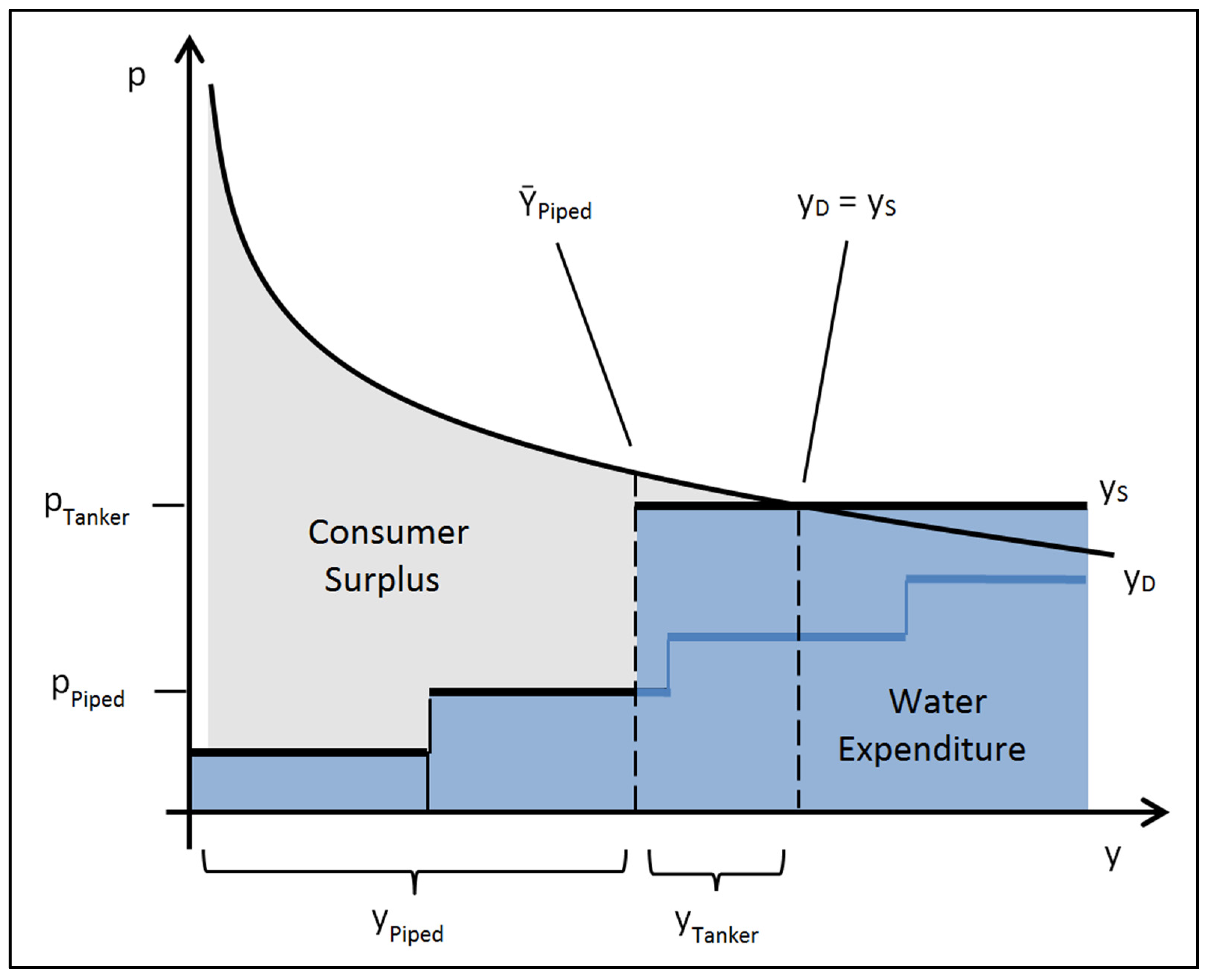
3. Model Concept

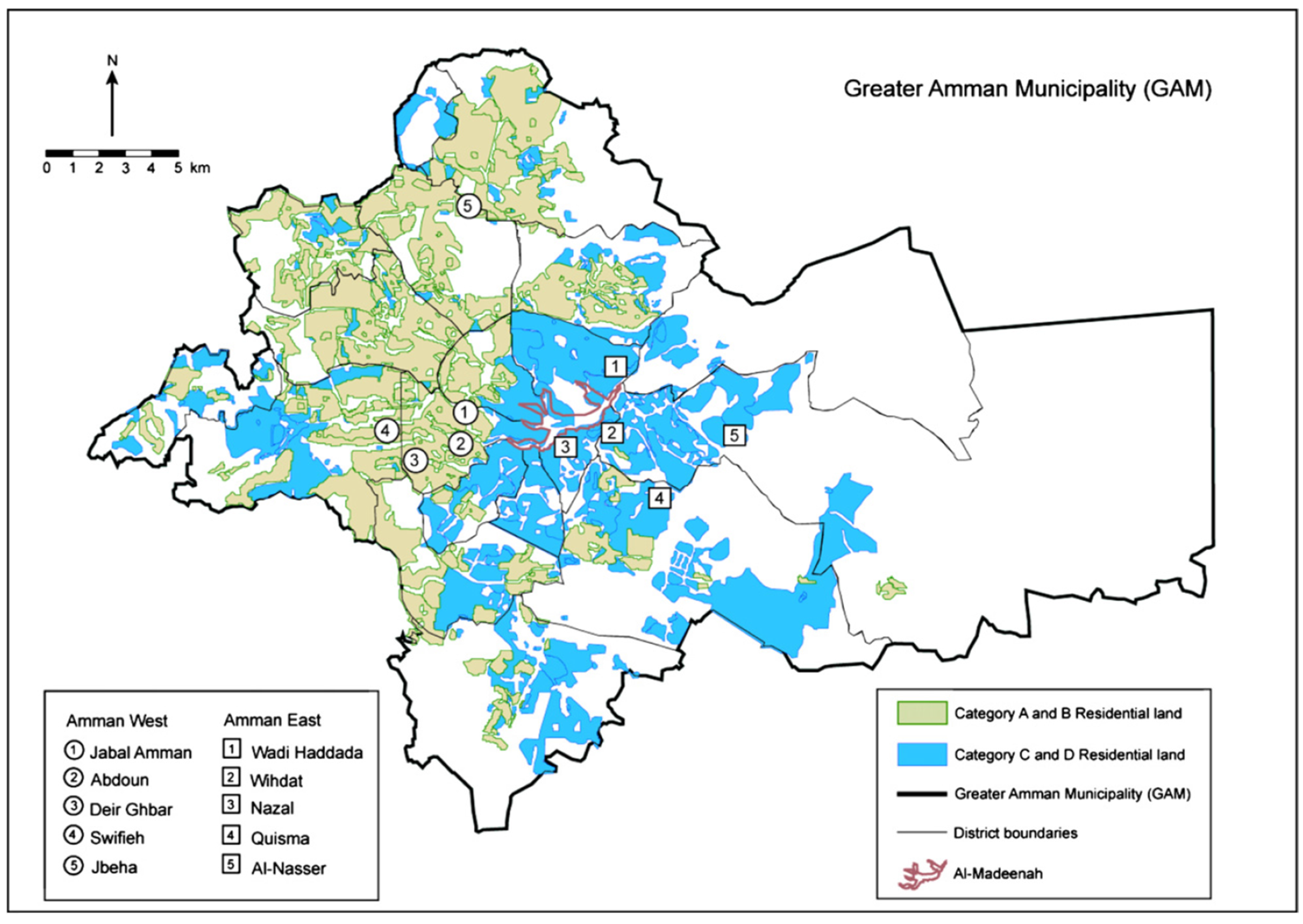
4. The Case Study: Household Water Supply and Consumption in the Greater Amman Municipality
5. Method

| Symbol | Explanation | Definition |
|---|---|---|
| Subscripts and Superscripts | ||
| Iteration number in the piped water distribution algorithm | ||
| District identifier | Al-Jameaa = 0, Al-Qwasmeh = 1, Marka = 2, Qasabet Amman = 3, Wadi Essier = 4 | |
| Income class identifier | high-income = 0, low-income = 1 | |
| Unique agent identifier | ||
| Variables | ||
| Total remaining piped water quantity in iteration of the distribution algorithm | ||
| Sum of connection days of the agents still dissatisfied in iteration of the distribution algorithm | ||
| Unconstrained piped water quantity demanded | ||
| Unconstrained piped water quantity demanded by tariff block | ||
| Piped water quantity demanded | ||
| Preliminary piped water quantity demanded in iteration of the distribution algorithm | ||
| Piped water quantity supplied | ||
| Tanker water quantity supplied | ||
| Consumer surplus difference to the baseline by agent | ||
| Total consumer surplus difference to the baseline | ||
| Symbol | Explanation | Definition | Source |
|---|---|---|---|
| Price elasticity of demand | [14] | ||
| Income elasticity of demand | [14] | ||
| Rate structure premium coefficient | [14] | ||
| Coefficient of household size | [14] | ||
| Coefficient of education | [14] | ||
| Coefficient of the house type | [14] | ||
| Coefficient of the number of bathrooms | [14] | ||
| Weekly supply duration by district in days | See Table A1 | [3] | |
| Number of households represented by agent | See Table A1 | [3] | |
| Tariffs by block in JD/m3, multiplied by the piped water tariff factor | [30] | ||
| Piped water tariff factor | (variable scenario parameter) | - | |
| Tanker water price in JD/m3 | [1,29,32] | ||
| Storage size by income class in m3 | [28] | ||
| Income by income class in JD/a | [28] | ||
| Rate structure premium by block in JD/day | [30] | ||
| Rate structure premium sample mean | (The actual RSP value differs from block to block. See explanation at the end of Section 5.1 for the reason for using a single RSP-value.) | [14] | |
| Household size (persons) | [33] | ||
| Household head’s level of education (Salman et al. [14] use the following definition: 1 = basic, 2 = secondary, 3 = diploma, 4 = university graduate, 5 = post graduate.) | [34] | ||
| House type (Salman et al. [14] use the following definition: 0 = house with garden, 1 = apartment or flat.) | [35] | ||
| Number of bathrooms in the household | [35] | ||
| Tariff structure block boundaries in m3/3 month | [30] | ||
| Total availability of piped water m3/day | [36] |
5.1. Piped Water Demand

5.2. Piped Water Allocation
| Algorithm 1. Piped water distribution algorithm. | |
| 1: | Set |
| 2: | Set |
| 3: | While |
| 4: | Loop across all household agents (m): |
| 5: | Set |
| 6: | If |
| 7: | Set |
| 8: | Update by setting it equal to its current value minus |
| 9: | Update by setting it equal to its current value minus |
| 10: | Else: |
| 11: | Set |
5.3. Tanker Water Consumption
5.4. Evaluation Variables
5.5. Implementation

5.6. Sensitivity Analyses

5.7. Additional Model Testing
5.8. Scenario Definitions
6. Results
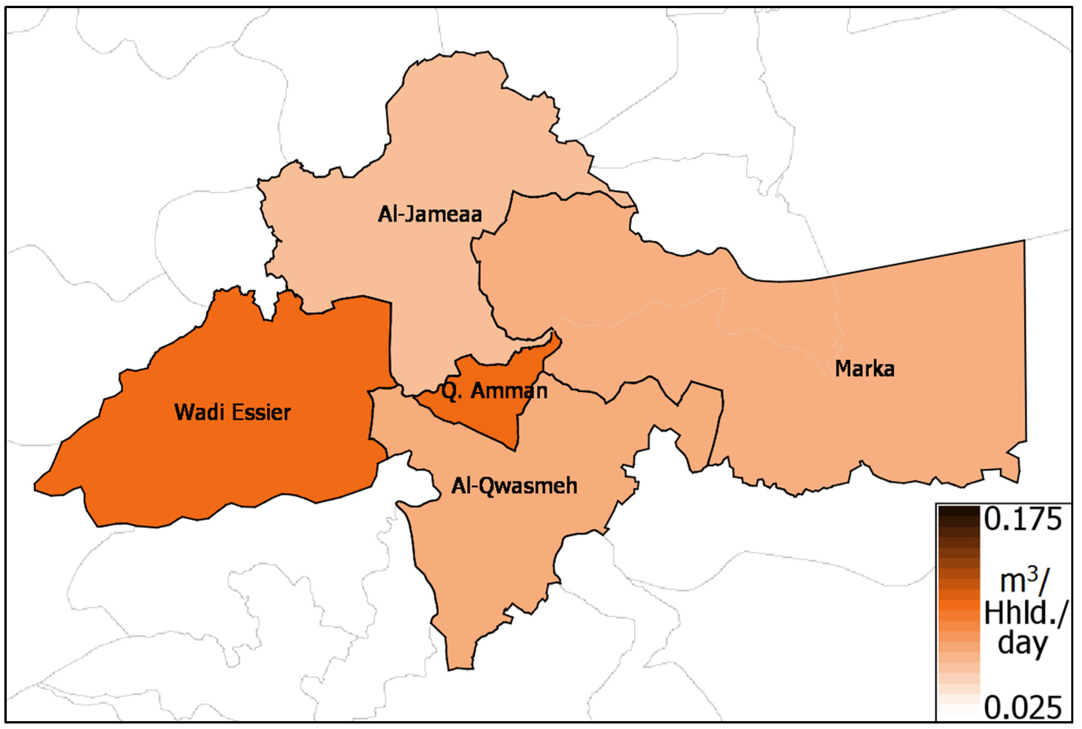
6.1. Analyses of Tanker Water Allocation
| Scenario | Al-Jameaa (Low) | Al-Jameaa (High) | Al-Qwasmeh (Low) | Al-Qwasmeh (High) | Marka (Low) | Marka (High) | Qasabet Amman (Low) | Qasabet Amman (High) | Wadi Essier (Low) | Wadi Essier (High) | Total (m3/day) |
|---|---|---|---|---|---|---|---|---|---|---|---|
| 1. Baseline | 0.057 | 0.064 | 0.066 | 0.077 | 0.065 | 0.080 | 0.100 | 0.113 | 0.099 | 0.11 | 38,451.163 |
| 2. = 1.925 | 0.076 | 0.091 | 0.089 | 0.106 | 0.092 | 0.109 | 0.123 | 0.137 | 0.126 | 0.147 | 50,938.482 |
| 3. = 7.7 | 0.044 | 0.051 | 0.048 | 0.058 | 0.046 | 0.055 | 0.08 | 0.091 | 0.081 | 0.091 | 29,453.320 |
| 4. = 0.1 | 0.068 | 0.082 | 0.080 | 0.096 | 0.083 | 0.098 | 0.112 | 0.125 | 0.113 | 0.133 | 45,953.797 |
| 5. = 0.5 | 0.058 | 0.068 | 0.069 | 0.081 | 0.069 | 0.084 | 0.103 | 0.115 | 0.101 | 0.115 | 39,952.404 |
| 6. = 2 | 0.051 | 0.059 | 0.058 | 0.069 | 0.054 | 0.068 | 0.092 | 0.104 | 0.092 | 0.103 | 34,363.630 |
| 7. Intermittency × 2 | 0.073 | 0.050 | 0.085 | 0.055 | 0.088 | 0.053 | 0.115 | 0.091 | 0.120 | 0.092 | 39,900.407 |
| 8. × 0.9 | 0.086 | 0.100 | 0.100 | 0.116 | 0.102 | 0.117 | 0.125 | 0.139 | 0.136 | 0.155 | 54,518.790 |
| Scenario | Al-Jameaa (Low) | Al-Jameaa (High) | Al-Qwasmeh (Low) | Al-Qwasmeh (High) | Marka (Low) | Marka (High) | Qasabet Amman (Low) | Qasabet Amman (High) | Wadi Essier (Low) | Wadi Essier (High) | Total (JD/Day) |
|---|---|---|---|---|---|---|---|---|---|---|---|
| 1. Baseline | 0 | 0 | 0 | 0 | 0 | 0 | 0 | 0 | 0 | 0 | 0 |
| 2. = 1.925 | 0.122 | 0.146 | 0.145 | 0.173 | 0.148 | 0.178 | 0.212 | 0.237 | 0.210 | 0.243 | 84,179 |
| 3. = 7.7 | −0.191 | −0.219 | −0.215 | −0.255 | −0.206 | −0.253 | −0.341 | −0.387 | −0.343 | −0.383 | −128,046 |
| 4. = 0.1 | 0.019 | 0.018 | −0.009 | −0.015 | 0 | 0.003 | 0.017 | 0.018 | −0.028 | −0.033 | 1282 |
| 5. = 0.5 | 0.033 | 0.032 | 0.023 | 0.021 | 0.023 | 0.023 | 0.026 | 0.026 | 0.015 | 0.012 | 11,694 |
| 6. = 2 | −0.054 | −0.053 | −0.033 | −0.032 | −0.029 | −0.032 | −0.031 | −0.037 | −0.024 | −0.016 | −16,397 |
| 7. Intermittency × 2 | −0.072 | 0.084 | −0.084 | 0.103 | −0.080 | 0.111 | −0.061 | 0.086 | −0.091 | 0.107 | −2292 |
| 8. × 0.9 | −0.116 | −0.123 | −0.140 | −0.152 | −0.128 | −0.130 | −0.100 | −0.107 | −0.147 | −0.154 | −60,474 |
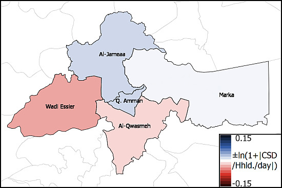
6.2. Analyses of Consumer Surplus Impacts

7. Discussion
8. Conclusions
Acknowledgments
Author Contributions
Conflicts of Interest
Appendix
| Al-Jameaa | Marka | Q. Amman | Al-Qwasmeh | Wadi Essier | ||||||||||
|---|---|---|---|---|---|---|---|---|---|---|---|---|---|---|
| Supply Duration (h/week) | No. of Households | Supply Duration (h/week) | No. of Households | Supply Duration (h/week) | No. of Households | Supply Duration (h/week) | No. of Households | Supply Duration (h/week) | No. of Households | |||||
| High Income | Low Income | High Income | Low Income | High Income | Low Income | High Income | Low Income | High Income | Low Income | |||||
| 24 | 5261 | 477 | 23 | 513 | 2450 | 23 | 1000 | 1282 | 29 | 2069 | 5222 | 24 | 4381 | 3557 |
| 27 | 118 | 11 | 24 | 539 | 2574 | 24 | 4379 | 5610 | 31 | 6491 | 16,383 | 28 | 6934 | 5630 |
| 29 | 3551 | 322 | 25 | 920 | 4397 | 25 | 1795 | 2300 | 32 | 420 | 1060 | 32 | 102 | 83 |
| 30 | 7000 | 635 | 27 | 26 | 126 | 27 | 214 | 274 | 36 | 4798 | 12,111 | 35 | 220 | 178 |
| 32 | 6282 | 570 | 29 | 918 | 4385 | 28 | 3341 | 4280 | 42 | 664 | 1676 | 48 | 8871 | 7203 |
| 35 | 4177 | 379 | 30 | 1917 | 9159 | 29 | 6416 | 8220 | 48 | 6208 | 15,670 | 62 | 2200 | 1786 |
| 36 | 636 | 58 | 32 | 390 | 1863 | 31 | 11,283 | 14,455 | 51 | 632 | 1595 | 70 | 210 | 171 |
| 48 | 23,500 | 2132 | 33 | 1635 | 7812 | 32 | 761 | 974 | 54 | 798 | 2015 | |||
| 61 | 1931 | 175 | 35 | 1604 | 7664 | 35 | 878 | 1125 | 55 | 361 | 910 | |||
| 62 | 13,805 | 1252 | 42 | 908 | 4336 | 36 | 490 | 627 | 57 | 3686 | 9305 | |||
| 68 | 8 | 1 | 44 | 5533 | 26,437 | 48 | 165 | 211 | 60 | 244 | 616 | |||
| 70 | 1321 | 120 | 48 | 1619 | 7735 | 51 | 2000 | 2562 | 61 | 785 | 1982 | |||
| 72 | 7108 | 645 | 61 | 109 | 521 | 54 | 2526 | 3236 | 80 | 852 | 2151 | |||
| 144 | 2012 | 183 | 62 | 188 | 899 | 57 | 1793 | 2296 | 120 | 114 | 289 | |||
| 68 | 4 | 17 | 60 | 773 | 990 | 126 | 727 | 1834 | ||||||
| 70 | 18 | 86 | 61 | 2485 | 3184 | |||||||||
| 73 | 603 | 2880 | 62 | 891 | 1141 | |||||||||
| 78 | 1653 | 7898 | 70 | 85 | 109 | |||||||||
| 80 | 2349 | 11,223 | 73 | 545 | 698 | |||||||||
| 102 | 860 | 4107 | 126 | 6899 | 8838 | |||||||||
| 120 | 315 | 1507 | 168 | 4091 | 5241 | |||||||||
| 144 | 114 | 543 | ||||||||||||
| 168 | 106 | 506 | ||||||||||||
References and Notes
- Rosenberg, D.E.; Talozi, S.; Lund, J.R. Intermittent water supplies: Challenges and opportunities for residential water users in Jordan. Water Int. 2008, 33, 488–504. [Google Scholar] [CrossRef]
- The term “non-observed” has been introduced by an OECD handbook on the topic to more precisely define parts of the economy also referred to as: “hidden economy, shadow economy, parallel economy, subterranean economy, informal economy, cash economy, black market”, etc. See: Organization for Economic Co-operation and Development (OECD). Measuring the Non-Observed Economy; OECD: Paris, France, 2002; Available online: http://www.oecd.org/std/na/1963116.pdf (accessed on 25 May 2015).
- Abu Amra, B.; Al-A’raj, A.; Al Atti, N.; Dersieh, T.; Hanieh, R.; Hendi, S.; Homoud, F.; Hussein, Y.; Jaloukh, R.; Rayyan, N. Amman Water Supply Planning Report, Volume 3, Appendices G & H; Report prepared by CDM for the United States Agency for International Development (USAID), the Ministry of Water and Irrigation (MWI), and the Water Authority of Jordan (WAJ); USAID: Amman, Jordan, 2011. [Google Scholar]
- Jordan Water Project. Available online: https://pangea.stanford.edu/researchgroups/jordan/ (accessed on 25 May 2015).
- Ministry of Water and Irrigation (MWI). Water for Life—Jordan’s Water Strategy 2008–2022; MWI: Amman, Jordan, 2009.
- United Nations Development Programme (UNDP). Human Development Report 2006: Beyond Scarcity—Power, Poverty and the Global Water Crisis; Palgrave Macmillan: New York, NY, USA, 2006. [Google Scholar]
- Kubursi, A.; Grover, V.; Darwish, A.R.; Deutsch, E. Water Scarcity in Jordan: Economic Instruments, Issues and Options; The Economic Research Forum (ERF) Working Paper 599; ERF: Cairo, Egypt, 2011. [Google Scholar]
- Ministry of Planning and International Cooperation and United Nations (MPIC and UN). Needs Assessment Review of the Impact of the Syrian Crisis on Jordan; Host Community Support Platform (HCSP) Report. HCSP: Amman, Jordan, 2013. Available online: http://www.hcspjordan.org/s/Needs-Assessment-Review_Jordan.pdf (accessed on 25 May 2015).
- Bonn, T. On the political sideline? The institutional isolation of donor organizations in Jordanian hydropolitics. Water Policy 2013, 15, 728–737. [Google Scholar] [CrossRef]
- Humpal, D.; El-Naser, H.; Irani, K.; Sitton, J.; Renshaw, K.; Gleitsmann, B. Review of Water Policies in Jordan and Recommendations for Strategic Priorities: Final report; United States Agency for International Development (USAID): Washington, DC, USA, 2012.
- French Development Agency (FDA/AFD). Jordan Water Demand Management Study; Report prepared for the Ministry of Water and Irrigation of Jordan (MWI). FDA/AFD: Paris, France, 2011. Available online: http://cmimarseille.org/cmiarchive/_src/EW2_wk1/EW2_wk1_JordanFinalReport.pdf (accessed on 25 May 2015).
- Yorke, V. Politics Matter: Jordan’s Path to Water Security Lies through Political Reforms and Regional Cooperation; Swiss National Centre of Competence in Research (NCCR) Working Paper No. 2013/19; NCCR: Bern, Switzerland, 2013. [Google Scholar]
- Al-Kharabsheh, A.; Ta’any, R. Challenges of Water Demand Management in Jordan. Water Int. 2005, 30, 210–219. [Google Scholar] [CrossRef]
- Salman, A.; Al-Karablieh, E.K.; Haddadin, M.A. Limits of pricing policy in curtailing household water consumption under scarcity conditions. Water Policy 2008, 10, 295–304. [Google Scholar] [CrossRef]
- Tabieh, M.; Salman, A.; Al-Karablieh, E.; Al-Qudah, H.; Al-Khatib, H. The Residential Water Demand Function in Amman-Zarka Basin in Jordan. Wulfenia J. 2012, 19, 324–333. [Google Scholar]
- Coulibaly, L.; Jakus, P.M.; Keith, J.E. Modeling water demand when households have multiple sources of water. Water Resour. Res. 2014, 50, 6002–6014. [Google Scholar] [CrossRef]
- Kariuki, M.; Schwartz, J. Small-Scale Private Service Providers of Water Supply and Electricity: A Review of Incidence, Structure, Pricing and Operating Characteristics; World Bank Policy Research Working Paper 3727; World Bank: Washington, DC, USA, 2005. [Google Scholar]
- Opryszko, M.C.; Huang, H.; Soderlund, K.; Schwab, K.J. Data gaps in evidence-based research on small water enterprises in developing countries. J. Water Health 2009, 7, 609–622. [Google Scholar] [CrossRef] [PubMed]
- Rosenberg, D.E.; Tarawneh, T.; Abdel-Khaleq, R.; Lund, J.R. Modeling integrated water user decisions in intermittent supply systems. Water Resour. Res. 2007, 43. [Google Scholar] [CrossRef]
- Srinivasan, V.; Gorelick, S.M.; Goulder, L. Sustainable urban water supply in south India: Desalination, efficiency improvement, or rainwater harvesting? Water Resour. Res. 2010, 46. [Google Scholar] [CrossRef]
- Srinivasan, V.; Gorelick, S.M.; Goulder, L. Factors determining informal tanker water markets in Chennai, India. Water Int. 2010, 35, 254–269. [Google Scholar] [CrossRef]
- Page, S.E. Agent-based models. In The New Palgrave Dictionary of Economics, 2nd ed.; Durlauf, S.N., Blume, L.E., Eds.; Palgrave Macmillan: London, UK, 2008; Available online: http://www.dictionaryofeconomics.com/article?id=pde2008_A000218 (accessed on 25 May 2015).
- Epstein, J.M. Generative Social Science: Studies in Agent-Based Computational Modeling; Princeton University Press: Princeton, NJ, USA, 2006; pp. 4–46. [Google Scholar]
- Department of Statistics (DOS). Jordan Statistical Yearbook 2013; Issue No. 64; DOS: Amman, Jordan, 2013. Available online: http://www.dos.gov.jo/ (accessed on 25 May 2015).
- Ministry of Water and Irrigation and Ministry of Planning and International Cooperation (MWI and MPIC). Quantification of the Impact of Syrian Refugees on the Water Sector in Jordan. In Proceedings of the High Level Conference on Jordan’s Water Crisis, Amman, Jordan, 2 December 2013; MWI: Amman, Jordan, 2013. [Google Scholar]
- Potter, R.B.; Darmame, K.; Barham, N.; Nortcliff, S. “Ever-growing Amman”, Jordan: Urban expansion, social polarisation and contemporary urban planning issues. Habitat Int. 2009, 33, 81–92. [Google Scholar] [CrossRef]
- Potter, R.B.; Darmame, K.; Nortcliff, S. Issues of water supply and contemporary urban society: the case of Greater Amman, Jordan. Philos. Trans. R. Soc. A Math. Phys. Eng. Sci. 2010, 368, 5299–5313. [Google Scholar] [CrossRef] [PubMed]
- Potter, R.B.; Darmame, K. Contemporary social variations in household water use, management strategies and awareness under conditions of “water stress”: The case of Greater Amman, Jordan. Habitat Int. 2010, 34, 115–124. [Google Scholar] [CrossRef]
- Gerlach, E.; Franceys, R. Regulating water services for the poor: The case of Amman. Geoforum 2009, 40, 431–441. [Google Scholar] [CrossRef]
- Water Authority of Jordan (WAJ). Water and Wastewater Tariff for Quarterly Bills for Governorates which are Managed by Companies 2012; WAJ: Amman, Jordan, 2012. Available online: http://www.waj.gov.jo/ (accessed on 25 May 2015).
- Theodory, G. Willingness and Ability of Residential and Non-Residential Subscribers in Greater Amman to Pay More for Water: A Study Conducted for the Water Authority of Jordan; Prepared for the United States Agency for International Development (USAID); Development Alternatives, Inc. (DAI): Amman, Jordan, 2000; p. 237. Available online: http://pdf.usaid.gov/pdf_docs/pnacq616.pdf (accessed on 25 May 2015).
- Wildmann, T. Water Market System in Balqa, Zarqa,& Informal Settlements of Amman & the Jordan Valley—Jordan; Oxfam: Oxford, UK, 2013. [Google Scholar]
- Department of Statistics (DOS). Table 3.12: Average Annual Current Income of Household Member by Source, Governorate and Urban/Rural (in JD). In Household Expenditure & Income Survey 2010; DOS: Amman, Jordan, 2010. Available online: http://www.dos.gov.jo/ (accessed on 25 May 2015). [Google Scholar]
- Department of Statistics (DOS). Table 4.2: Distribution of Jordanian Population Living in Jordan Aged 5-29 Years Who Enrolled in Educational Institutions by Grade, Educational Stage, Sex and Governorates. In Population and Housing Census 2004; DOS: Amman, Jordan, 2004. Available online: http://www.dos.gov.jo/ (accessed on 25 May 2015). [Google Scholar]
- Al-Najjar, F.O.; Al-Karablieh, E.K.; Salman, A. Residential Water Demand Elasticity in Greater Amman Area. Jordan J. Agric. Sci. 2011, 7, 93–103. [Google Scholar]
- Miyahuna. Customer Demand Profile; Miyahuna: Amman, Jordan, 2008. [Google Scholar]
- GIMP Home Page. Available online: http://www.gimp.org/ (accessed on 25 May 2015).
- Potter, R.B.; Darmame, K. Contemporary social variations in household water use, management strategies and awareness under conditions of “water stress”: The case of Greater Amman, Jordan. Habitat Int. 2010, 34, 115–124, (118). [Google Scholar] [CrossRef]
- Taylor, L.D. The Demand for Electricity: A Survey. Bell J. Econ. 1975, 6, 74–110. [Google Scholar] [CrossRef]
- Nordin, J.A. A proposed modification of Taylor’s demand analysis: Comment. Bell J. Econ. 1976, 7, 719–721. [Google Scholar] [CrossRef]
- Billings, R.B.; Agthe, D.E. Price elasticities for water: A case of increasing block rates. Land Econ. 1980, 56, 73–84. [Google Scholar] [CrossRef]
- Wilensky, U. NetLogo; Center for Connected Learning and Computer-Based Modeling. Northwestern University: Evanston, IL, USA, 1999. Available online: http://ccl.northwestern.edu/netlogo/ (accessed on 25 May 2015).
- Mulligan, M.; Wainwright, J. Modelling and Model Building. In Environmental Modelling: Finding Simplicity in Complexity; Wainwright, J., Mulligan, M., Eds.; John Wiley and Sons: Chichester, UK, 2004; pp. 7–74. [Google Scholar]
© 2015 by the authors; licensee MDPI, Basel, Switzerland. This article is an open access article distributed under the terms and conditions of the Creative Commons Attribution license (http://creativecommons.org/licenses/by/4.0/).
Share and Cite
Klassert, C.; Sigel, K.; Gawel, E.; Klauer, B. Modeling Residential Water Consumption in Amman: The Role of Intermittency, Storage, and Pricing for Piped and Tanker Water. Water 2015, 7, 3643-3670. https://doi.org/10.3390/w7073643
Klassert C, Sigel K, Gawel E, Klauer B. Modeling Residential Water Consumption in Amman: The Role of Intermittency, Storage, and Pricing for Piped and Tanker Water. Water. 2015; 7(7):3643-3670. https://doi.org/10.3390/w7073643
Chicago/Turabian StyleKlassert, Christian, Katja Sigel, Erik Gawel, and Bernd Klauer. 2015. "Modeling Residential Water Consumption in Amman: The Role of Intermittency, Storage, and Pricing for Piped and Tanker Water" Water 7, no. 7: 3643-3670. https://doi.org/10.3390/w7073643
APA StyleKlassert, C., Sigel, K., Gawel, E., & Klauer, B. (2015). Modeling Residential Water Consumption in Amman: The Role of Intermittency, Storage, and Pricing for Piped and Tanker Water. Water, 7(7), 3643-3670. https://doi.org/10.3390/w7073643