Daily Reservoir Runoff Forecasting Method Using Artificial Neural Network Based on Quantum-behaved Particle Swarm Optimization

Abstract

Accurate daily runoff forecasting is of great significance for the operation control of hydropower station and power grid. Conventional methods including rainfall-runoff models and statistical techniques usually rely on a number of assumptions, leading to some deviation from the exact results. Artificial neural network (ANN) has the advantages of high fault-tolerance, strong nonlinear mapping and learning ability, which provides an effective method for the daily runoff forecasting. However, its training has certain drawbacks such as time-consuming, slow learning speed and easily falling into local optimum, which cannot be ignored in the real world application. In order to overcome the disadvantages of ANN model, the artificial neural network model based on quantum-behaved particle swarm optimization (QPSO), ANN-QPSO for short, is presented for the daily runoff forecasting in this paper, where QPSO was employed to select the synaptic weights and thresholds of ANN, while ANN was used for the prediction. The proposed model can combine the advantages of both QPSO and ANN to enhance the generalization performance of the forecasting model. The methodology is assessed by using the daily runoff data of Hongjiadu reservoir in southeast Guizhou province of China from 2006 to 2014. The results demonstrate that the proposed approach achieves much better forecast accuracy than the basic ANN model, and the QPSO algorithm is an alternative training technique for the ANN parameters selection.

1. Introduction

Accurate daily runoff forecasting is extremely important for hydropower operation control and power grid operation scheduling [1,2,3,4,5]. Over the past decades, there have been abundant traditional classical research works for the daily runoff forecasting, which can be broadly separated into two categories: process-based model like Xin’anjiang model [6,7], and data-based model such as autoregressive model and moving average model [8,9]. These approaches entail exogenous input and rely on a number of assumptions for natural environment, leading to some deviation from the exact results in most cases. In recent years, with the booming development of heuristic methods, many researchers pay attention to applying them in daily runoff forecasting or the parameter selection of the hydrologic model, including artificial neural network [10,11], SCE-UA algorithm [12,13], support vector machine [14,15] and other hybrid methods [16,17].

As a typical artificial neural network, back propagation neural network (BP) can nearly simulate any complex linear or non-linear functional relationship without knowing the correlation between the input data and the output data [18,19]. After learning from the training data set, BP can be used to predict a new output data effectively with the corresponding input data. Compared with other methods, BP has high fault tolerance, strong robustness and easy adaptability to online learning. BP has been widely used in many practical areas, including load prediction, wind speed prediction and daily runoff forecasting. However, BP has some drawbacks, such as long computing time, slow convergence and easy to encounter local minimum. Hence, a variety of hybrid optimization methods using such global optimization algorithm like particle swarm optimization (PSO) are developed to improve the generalization ability of the artificial neural network [20,21]. These hybrid optimization methods can improve the BP forecasting performance in varying degrees. However, when PSO is applied for the ANN parameters selection, it may be trapped into the local optima of the objective function because PSO is restricted by search capability. Therefore, the promotion space is still large for ANN parameter selection using an evolutionary algorithm [22,23,24].

In recent years, a novel particle swarm optimization variant called quantum-behaved particle swarm optimization algorithm (QPSO) was proposed by Sun et al. [25] in 2004. In QPSO, the global optimal solution in the whole searching space can be guaranteed theoretically. Moreover, simulation results of numerous complex benchmark functions showed that QPSO has better global searching ability than the basic PSO [26,27]. Hence, QPSO are widely used to solve the complex optimization problems which includes hydrothermal scheduling and economic dispatch problem [28,29]. However, up to now, there are a few reports about using QPSO for parameter calibration of artificial neural network. Therefore, to improve the generalization ability and calculation efficiency of artificial neural network, a hybrid method, coupling artificial neural network and QPSO, is developed for daily reservoir runoff forecasting in this research, where QPSO algorithm is selected as training algorithm for artificial neural network to enhance hydrologic forecast accuracy.

The remaining is organized as follows. Artificial neural network is introduced briefly in Section 2. Section 3 explains the PSO and QPSO methods in details, then the proposed QPSO-ANN model is presented in Section 4. Section 5 provides the results of the proposed method and other methods and gives discussions on their performances. Finally, conclusions are summarized in Section 6.

2. Artificial Neural Network

In general, the relation between input vector and output vector of a nonlinear system can be expressed as Y = H(X), where X = [X₁,…,X_i,…,X_n]^T is input vector; X_i is the ith input data; n is the number of input data; Y = [Y₁,…,Y_j,…,Y_u]^T is output vector; Y_j is the jth input data; u is the number of output data; H(·) denotes the complex nonlinear relation which can be estimated by some meta-heuristic methods like artificial neural network.

In our study, BP neural network is chosen as the basic approach to estimate input-output relations H(·) of the nonlinear hydrological system. The main advantage of BP is that it can reflect the complex nature of underlying process with less information than other traditional methods. A typical BP neural network consists of three layers, input layer, hidden layer and output layer, whose structure is shown in Figure 1. Each layer is composed of a series of interconnected processing nodes. As a specific neuron, each node in any layer uses a nonlinear transfer function to calculate the inner product of input vector and weight vector to get a scalar result. Two neighboring layers are connected via the weights of the nodes between these layers. The input layer receives and transmits input data to hidden layer. The hidden layer may contain a single layer or multi-layer that receives values from the previous layer. Each hidden layer is responsible for the input information conversion and then delivers them to the next hidden layer or output layer. The output layer presents the simulated results and has only one single layer with one or several nodes. In a single calculation, the BP neural network can obtain overall error between the estimated output values and the target output values, then loss function gradient is calculated. The gradient-descent algorithm is fed to update weights and thresholds to minimize loss function. The connection weights and thresholds between any two feed forward-connected neurons will be unceasingly adjusted until the error meets the termination conditions. Then, the optimized BP neural network can be used to forecast the target value with the corresponding input vector.

Figure 1. Schematic diagram of three-layer back propagation (BP) neural network.

Figure 1. Schematic diagram of three-layer back propagation (BP) neural network.

Due to the defects of gradient descent method, the result may find a locally optimal solution instead of global optimum in most cases due to the existence of many local optima on the error surface. The convergence in back propagation learning cannot be guaranteed. Moreover, the computation speed is rather slow because the gradient descent algorithm requires small learning rates for stable learning.

3. Quantum-Behaved Particle Swarm Optimization

3.1. Particle Swarm Optimization

Particle Swarm Optimization (PSO), proposed by Kennedy and Eberhart in 1995 [30], is a well-known evolutionary population-based algorithm for global optimization problems [31,32]. The main concept of PSO is from analogy of biological and sociological feeding behavior of bird swarm, and its basic variant is a population (called a swarm) of candidate solutions (called particles). PSO is initialized with random solutions which search for optima by flying through problem space from generation to generation. The flight of each particle is guided continuously by its own best known position, pbest, and the best known position of the whole population, gbest. Each particle has position vector and velocity vector, and explores in the searching space by a few simple formulas.

There is extensive and profound homology or resemblance between PSO and other evolutionary computation techniques like genetic algorithm. Compared with genetic algorithm, PSO has faster convergence speed since it has no evolution operators like crossover and selection. Moreover, PSO has few parameters to adjust and depends directly upon function values rather than derivative information. In the past few years, PSO has been successfully applied to many research and application areas. However, the main defect of PSO is that global convergence cannot be guaranteed, especially when the number of decision variables or dimensions to be optimized are large. In other words, PSO is easily trapped into local optimum although it may have fast convergent rate [32,33].

3.2. Quantum-Behaved Particle Swarm Optimization

In order to deal with disadvantages of PSO, quantum-behaved particle swarm optimization (QPSO) was developed by Sun et al. [25] in 2004. From the quantum mechanics perspective, QPSO considers the particle possess quantum behavior and cannot determine the exact values of position vector and velocity vector simultaneously according to uncertainty principle [25,26]. Hence, there is no velocity vector in the particle of QPSO, and particle state is associated with an appropriate time-dependent Schrödinger equation and can be characterized by wave function ψ instead of position and velocity [27,28], where |ψ|² is the probability density function of its position. Let M particles in d dimensional space with $\overline{k}$ maximum generations, the position vector of ith particle at kth generation can be expressed as x_i(k) = [x_i,1(k),x_i,2(k),…,x_i,d(k)]^T. There will be gbest(k) = [gbest₁(k),gbest₂(k),…,gbest_d(k)]^T and pbest_i(k) = [pbest_i,1(k),pbest_i,2(k),…,pbest_i,d(k)]^T. Employing Monte-Carlo method, particle moves according to the following iterative equation:

$$x_{i,j}\left(k+\text{1}\right)=\{\begin{array}{l}{p}_{i,j}\left(k\text{+}1\right)+a\left(k\right)\times \left|mbes{t}_j\left(k+1\right)-x_{i,j}\left(k\right)\right|\times \text{ln}\left(\text{1}/r_1\right),if{r}_2\ge 0.5\\ p_{i,j}\left(k\text{+}1\right)-a\left(k\right)\times \left|mbes{t}_j\left(k+1\right)-x_{i,j}\left(k\right)\right|\times \text{ln}\left(\text{1}/r_1\right),if{r}_2<0.5\end{array}$$

(1)

$$p_{i,j}\left(k\text{+}1\right)=r_3\times pbes{t}_{i,j}\left(k\right)+\left(1-r_3\right)\times gbes{t}_j\left(k\right)$$

(2)

$$mbes{t}_j\left(k\text{+}1\right)\text{=}\frac{1}{M}{\displaystyle \sum _{i=1}^{M}pbes{t}_{i,j}\left(k\right)}$$

(3)

$$a\left(k\right)=\frac{\left(a_1-a_2\right)\times \left(\overline{k}-k\right)}{\overline{k}}+a_2$$

(4)

for i = 1,2,...,M; j = 1,2,...,d; k = 1,2,..., $\overline{k}$. Where x_i,j(k) is position for jth dimension of ith particle in kth generation; r₁, r₂, r₃ are random variables distributed uniformly in [0,1]; a(k) is contraction-expansion coefficient in kth generation which controls the convergence speed of the particle; a₁, a₂ are maximum and minimum value of a(k), respectively; and there are usually a₁ = 1.0, a₂ = 0.5 [28]; p_i,j(k) is the jth dimension of local attractor i in kth generation; mbest represents the mean best position defined as mean of all pbest position of the whole population.

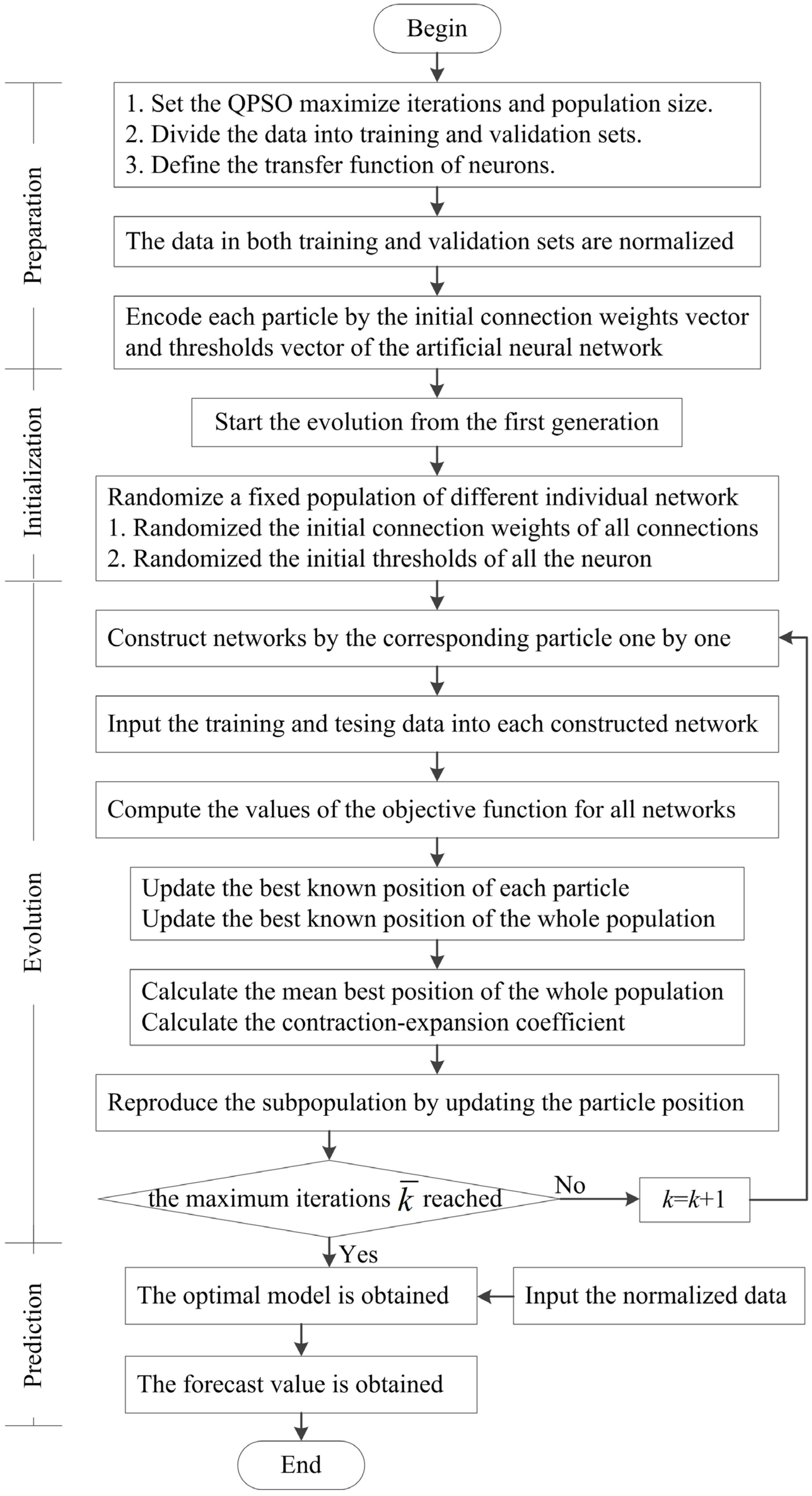
4. Parameters Selection for Artificial Neural Network Based on QPSO Algorithm

In order to obtain better forecast accuracy, the novel QPSO algorithm is employed for parameters selection of BP neural network. In this paper, there is only one node in output layer, which is the daily runoff forecast value. If the node number of input layer and hidden layer are n and m, respectively, the architecture of the ANN neural network is n-m-1. The flow chart of the proposed method is shown in Figure 2, and the fundamental idea of the proposed method can be described as follows:

• Step 0: Set basic parameters for the proposed method.
• Step 0.1: Set maximize iterations $\overline{k}$ and population size M in QPSO.
• Step 0.2: Divide data into training and testing sets.
• Step 0.3: Define transfer function of neurons, which is a sigmoid function in this paper, i.e.:

  $$f\left[x\right]=\frac{1}{1+e^{-x}}$$

  (5)

Step 1: The input and output data in both training and testing sets are normalized to ensure the quality of forecast results.

$$X\text{=}\left\{X_i^{\text{'}}\right\}=a\times \frac{X_i-X_i^{\min }}{X_i^{\max }-X_i^{\min }}+b$$

(6)

where $X_i^{\text{'}}$ and X_i is the normalized value and real value of each vector, respectively; $X_i^{\min }$ and $X_i^{\max }$ are the minimum and maximum value of input or output arrays; a and b are the positive normalized parameters, respectively. Based on large numbers of numerical experiments, we found that when the variable a = 0.2 and b = 0.6 are adopted to normalize the raw data, the forecasting models performs better. Hence, we use the variable a = 0.2 and b = 0.6 for data normalization in this paper.

Step 2: The QPSO algorithm is employed to select the parameters of BP neural network. The ith particle in the kth generation is denoted by x_i(k) = {w_i, b_i}. Here, w_i and b_i represent the connection weights and bias matrix between any two layers of the BP neural network, respectively.

Step 3: Set k = 1, and initialize the parameters w and b of every particle randomly in the searching space, which are the connection weight and bias on each node, respectively.

Step 4: Use the parameters to calculate the fitness of each particle. Here, the fitness is the forecasting error between the output values and the target ones.

Step 4.1: Calculate the outputs of all hidden layer nodes for each training sample.

$$y_j=f\left[{\displaystyle \sum _{i=1}^n{x}_i{w}_{ji}+b_j}\right],j=1,2,\cdots ,m$$

(7)

where w_ji represents the connection weight from the input node i to the hidden node j, b_j stands for bias of neuron j, y_j is the output value of the hidden layer node j.

Step 4.2: Calculate the output data of the BP neural network for each training sample.

$$o_1=f\left[{\displaystyle \sum _{j=1}^m{y}_i{w}_{1j}+b_1}\right]$$

(8)

where w_1j represent the connection weight from hidden node j to the output node 1, b₁ stands for the bias of the neuron; o₁ stands for the output data of network.

Step 4.3: Step 4.1 and 4.2 are repeated until all the training set samples are calculated. Then the forecasting error F is regarded as the fitness of the particle x_i(k).

$$F\left[x_i\left(k\right)\right]=\frac{1}{s}{\displaystyle \sum _{s=1}^S{\left(o_s-t_s\right)}^2}$$

(9)

where o_s and t_s is the sth normalized output value and target value in the training data, respectively. S is the number of training set samples.

Step 5: Update the best known position of each particle and the best known position of the whole population according to the following two formulas:

$$p_i\left(k\right)=\{\begin{array}{ll}{x}_i\left(k\right)& if(k=1)\\ \arg \min \left\{F\left[p_i\left(k-1\right)\right],F\left[x_i\left(k\right)\right]\right\}& otherwise\end{array}$$

(10)

$$gbest\left(k\right)=\{\begin{array}{ll}\arg \min \left\{\underset{1\le i\le M}{\min }\left\{F\left[p_i\left(k\right)\right]\right\},F\left[gbest\left(k-1\right)\right]\right\}& if(k>1)\\ \arg \min \left\{\underset{1\le i\le M}{\min }\left\{F\left[p_i\left(k\right)\right]\right\}\right\}& otherwise\end{array}$$

(11)

Step 6: Calculate the mean best position and the contraction-expansion coefficient with Equations (3) and (4), respectively.

Step 7: Update current position of each particle by the Equation (1).

Step 8: Set k = k+1, if the maximum iterations $\overline{k}$ reached, the flow will go to Step 9, else go back to Step 4.

Step 9: Output the optimal parameter of the BP neural network, which will be used for new data forecasting process.

Step 10: Before starting the forecasting process, the input vector are needed to be normalized by Equation (6), then transmit the processed data into the calibrated artificial neural network model to obtain predictive value. The predictive data need to be renormalized to the original range of output data by Equation (12).

$$\widehat{Y}\text{=}\left\{{\widehat{Y}}_i\right\}=\frac{\left(Y_i^{\text{'}}-b\right)\times \left(Y_i^{\max }-Y_i^{\min }\right)}{a}+Y_i^{\min }$$

(12)

where $Y_i^{\text{'}}$ and ${\widehat{Y}}_i$ are normalized forecasting value and real forecasting value of the output vector, respectively; $Y_i^{\min }$ and $Y_i^{\max }$ are minimum and maximum value of the output arrays, respectively.

Figure 2. Flow chart of the proposed method.

Figure 2. Flow chart of the proposed method.

5. Simulations

5.1. Study Area and Data Used

The study site is Hongjiadu reservoir in Wu River of Guizhou Province in southwest China. The Wu River is the biggest branch at southern bank of Yangtze River. Hongjiadu reservoir is the leading one with multi-year regulation ability of eleven cascade hydropower stations on Wu River. Rainfall produces most of the runoff. Its drainage area is 9900 km² and the mean annual runoff is 155 m³·s⁻¹ at the dam site. The total reservoir storage is 4.95 billion cubic meters and the regulated storage is 3.36 billion cubic meters. Locations of Wu River and Hongjiadu reservoir are shown in Figure 3.

Figure 3. Location of study area.

Figure 3. Location of study area.

All the daily runoff data collected from Hongjiadu reservoir operators is from 1 January 2006 to 31 December 2013. The data set between 1 January 2006 and 31 December 2012 is used for parameters calibration, while that from 1 January 2013 to 31 December 2013 is for testing. Moreover, before applying the proposed method for daily runoff predication, the data should be normalized to avoid numerical difficulties during calculation and guarantee consistency of greater numeric ranges as well as smaller ones. In the modeling process, input and output data sets are linearly scaled to [0.2, 0.8] as shown in Equation (6).

5.2. Performance Assessment Measures

Many performance measure methods have been developed to assess the forecast accuracy. However, so far, there is no unified standard since each measure can reflect one or more characteristics of the forecasting method. Hence, four commonly used metrics are selected to evaluate the forecast results: coefficient of correlation (R), Nash-Sutcliffe efficiency coefficient (NSE), root mean squared error (RMSE) and mean absolute percentage error (MAPE). R evaluates the linear relation between two data sequences, while NSE shows the capability of the model in predicting values away from the mean. The larger the value of R and NSE, the better the performances of the forecasting model. RMSE and MAPE measure the residual error and the mean absolute percentage error between the observed and forecasted data, respectively. The smaller the value of RMSE and MAPE, the better the performances of the forecasting model.

$$R={\displaystyle \sum _{i=1}^n\left[\left(Y_i-\overline{Y}\right)\left({\widehat{Y}}_i-\tilde{Y}\right)\right]}/\sqrt{{\displaystyle \sum _{i=1}^n{\left(Y_i-\overline{Y}\right)}^2{\left({\widehat{Y}}_i-\tilde{Y}\right)}^2}}$$

(13)

$$NSE=1-{\displaystyle \sum _{i=1}^n{\left(Y_i-{\widehat{Y}}_i\right)}^2}/{\displaystyle \sum _{i=1}^n{\left(Y_i-\overline{Y}\right)}^2}$$

(14)

$$RMSE=\sqrt{\frac{1}{n}{\displaystyle \sum _{i=1}^n{\left(Y_i-{\widehat{Y}}_i\right)}^2}}$$

(15)

$$MAPE=\frac{1}{n}{\displaystyle \sum _{i=1}^n\left|\frac{Y_i-{\widehat{Y}}_i}{Y_i}\right|}\times 100$$

(16)

where Y_i and ${\widehat{Y}}_i$ are the observed value and predictive value of ith data, respectively. $\overline{Y}$ and $\tilde{Y}$ represent the mean value of the observed value and predictive value, respectively. n is the total number of data set used for performance evaluation and comparison.

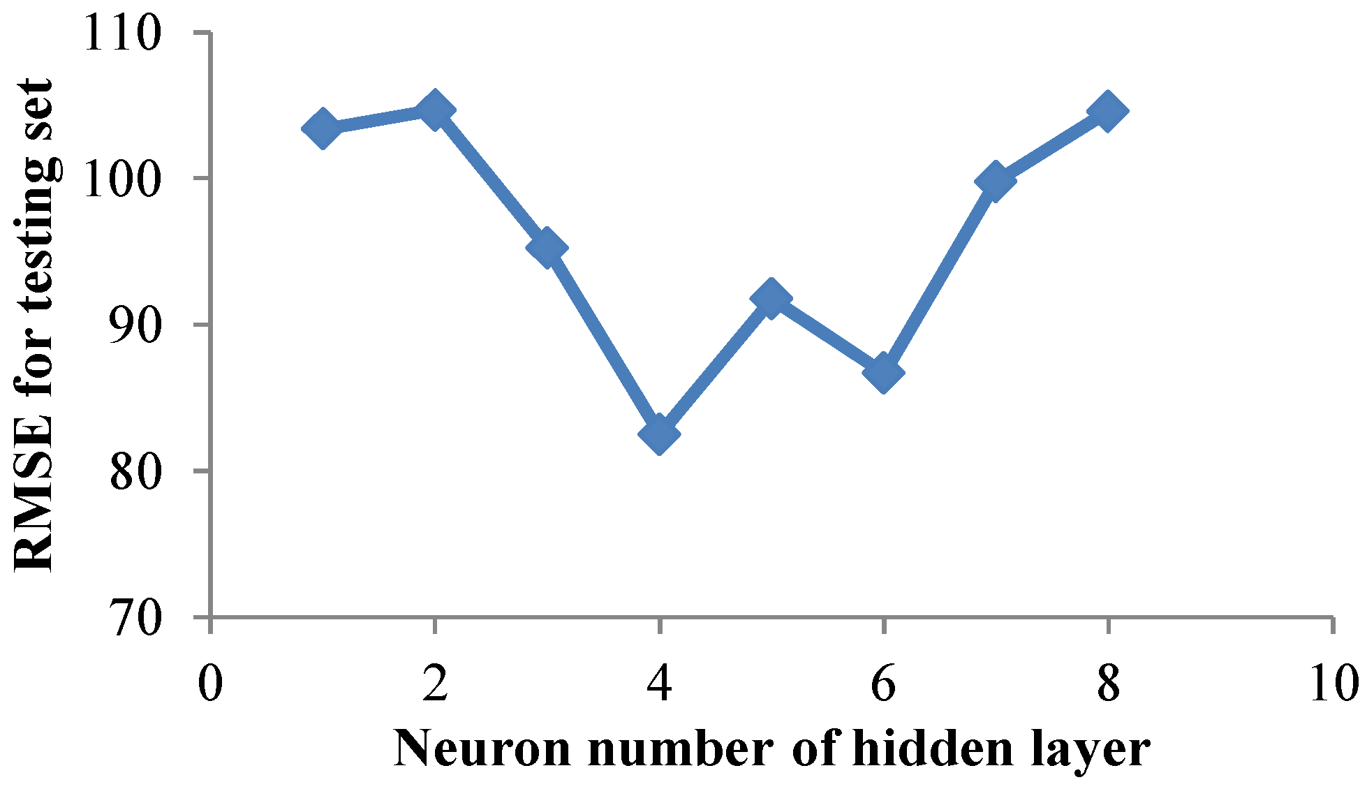
5.3. ANN Model Development

For ANN, proper selection of input variables will be helpful to find the best-fitted model. Based on the analysis of cross correlation coefficient and autocorrelation coefficient, four input combinations with different antecedent rainfalls and runoffs were developed for a comparative purpose. Table 1 summarizes these ANN models used for this study, where Runoff(t), Rainfall(t) are the runoff and rainfall value at the t-th period, respectively. To ensure the generalization capability of ANN, we use the trial and error method to determine the optimal network architecture. According to Chau et al. in 2005, the training process needs to be stopped when the error of the testing set starts to increase and that of the training set is still decreasing. Figure 4 shows the performance for the testing set against various numbers of neurons for model 1. The optimal ANN architecture adopted for model 1 is 2-4-1. The other three models have the same procedures as that for model 1. Table 2 shows the architecture and indices of various ANN forecasting models for Hongjiadu reservoir. We can find that antecedent two-day rainfalls and antecedent two-day runoff should be chosen as predictors, and ANN with the architecture of 4-7-1 performs best at this situation.

Table 1. Inputs and relation for various artificial neural network (ANN) forecasting models.

Model	Inputs	Relation between Output Variable and Input Variables
1	Runoff(t-1),Rainfall(t-1)	Runoff(t)=H[Runoff(t-1),Rainfall(t-1)]
2	Runoff(t-1),Rainfall(t-1),Rainfall(t-2)	Runoff(t)=H[Runoff(t-1),Rainfall(t-1),Rainfall(t-2)]
3	Runoff(t-1),Runoff(t-2),Rainfall(t-1)	Runoff(t)=H[Runoff(t-1),Runoff(t-2),Rainfall(t-1)]
4	Runoff(t-1),Runoff(t-2),Rainfall(t-1),Rainfall(t-2)	Runoff(t)=H[Runoff(t-1),Runoff(t-2),Rainfall(t-1),Rainfall(t-2)]

Table 1. Inputs and relation for various artificial neural network (ANN) forecasting models.

Model	Inputs	Relation between Output Variable and Input Variables
1	Runoff(t-1),Rainfall(t-1)	Runoff(t)=H[Runoff(t-1),Rainfall(t-1)]
2	Runoff(t-1),Rainfall(t-1),Rainfall(t-2)	Runoff(t)=H[Runoff(t-1),Rainfall(t-1),Rainfall(t-2)]
3	Runoff(t-1),Runoff(t-2),Rainfall(t-1)	Runoff(t)=H[Runoff(t-1),Runoff(t-2),Rainfall(t-1)]
4	Runoff(t-1),Runoff(t-2),Rainfall(t-1),Rainfall(t-2)	Runoff(t)=H[Runoff(t-1),Runoff(t-2),Rainfall(t-1),Rainfall(t-2)]

Figure 4. Performance of model 1 against different numbers of nodes in hidden layer.

Figure 4. Performance of model 1 against different numbers of nodes in hidden layer.

Table 2. Architectures and indices of various ANN forecasting models for Hongjiadu reservoir.

Model	Model Architecture	Training				Testing
		R	NSE	RMSE (m3·s−1)	MAPE (%)	R	NSE	RMSE (m3·s−1)	MAPE (%)
1	2-4-1	0.892	0.740	82.490	38.150	0.883	0.747	63.562	35.912
2	3-6-1	0.891	0.737	82.989	37.903	0.903	0.757	62.321	38.417
3	3-5-1	0.893	0.742	82.090	36.493	0.903	0.761	61.792	37.190
4	4-7-1	0.907	0.783	75.286	34.866	0.904	0.773	60.252	35.680

Table 2. Architectures and indices of various ANN forecasting models for Hongjiadu reservoir.

Model	Model Architecture	Training				Testing
		R	NSE	RMSE (m3·s−1)	MAPE (%)	R	NSE	RMSE (m3·s−1)	MAPE (%)
1	2-4-1	0.892	0.740	82.490	38.150	0.883	0.747	63.562	35.912
2	3-6-1	0.891	0.737	82.989	37.903	0.903	0.757	62.321	38.417
3	3-5-1	0.893	0.742	82.090	36.493	0.903	0.761	61.792	37.190
4	4-7-1	0.907	0.783	75.286	34.866	0.904	0.773	60.252	35.680

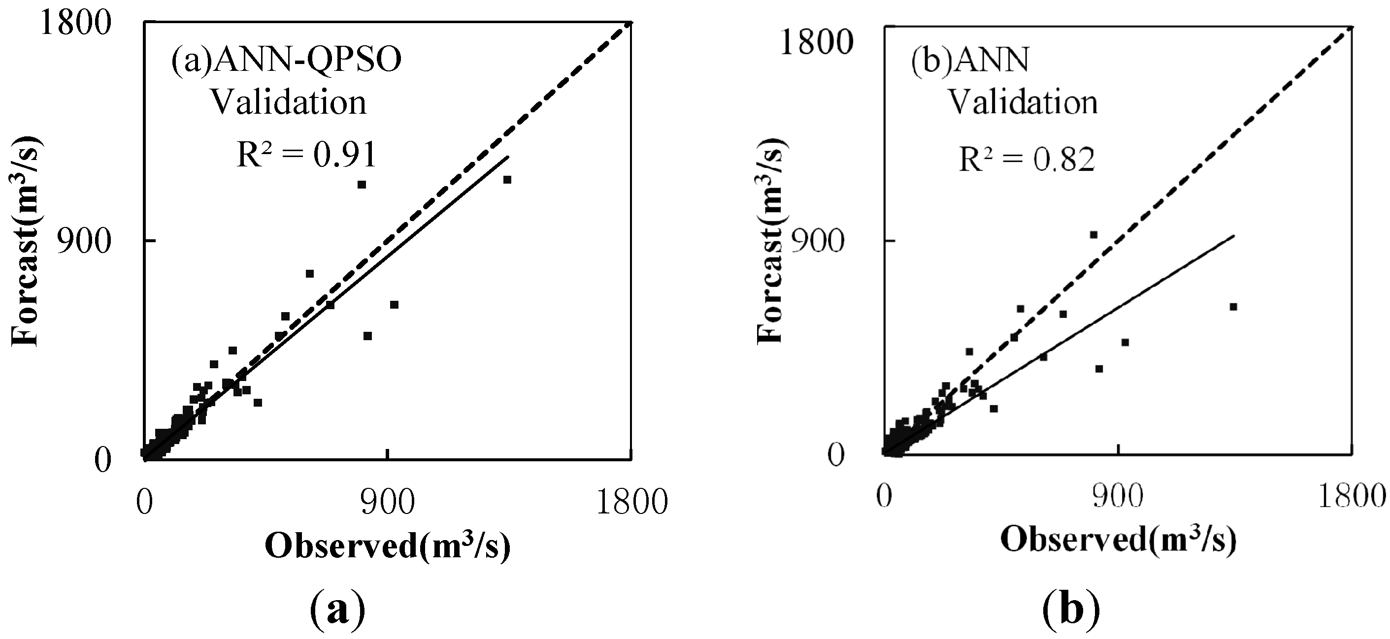
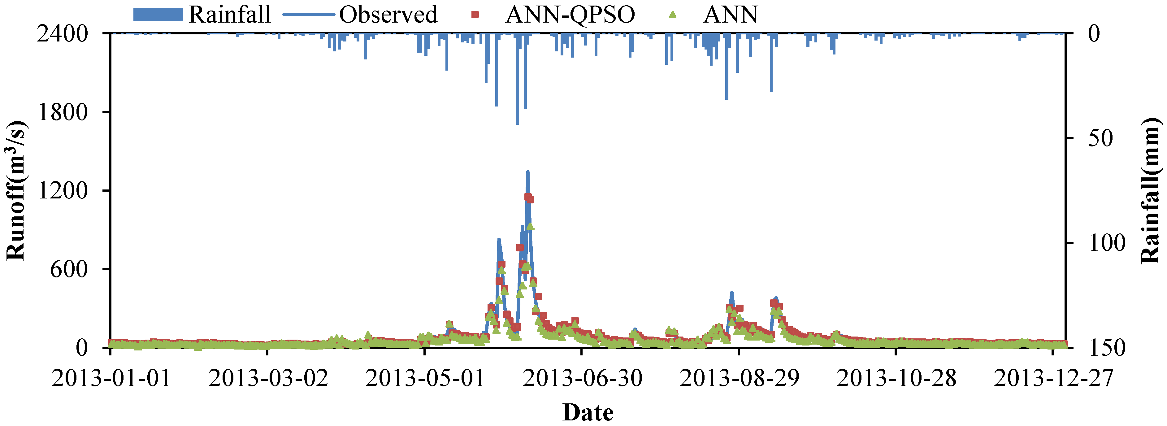
5.4. Comparison of Different Methods

In order to verify the effectiveness of the proposed method, the same training and verification samples are used for these two models, ANN and ANN-QPSO, and the above four quantitative indexes are employed to evaluate their performances. According to the above-mentioned analysis, the neural network architectures of both ANN and ANN-QPSO are 4-7-1 for Hongjiadu reservoir. Moreover, for ANN-QPSO, the number of population is set to be 300 whilst the maximize iterations is 500. The two algorithms are implemented by adopting JAVA language.

Table 3 presents the statistics results using various models developed for Hongjiadu study area. It can be seen that these two methods have different performances during both training and testing periods. Compared to the basic ANN, the proposed method is able to produce better forecast results for the daily runoff forecasting in Hongjiadu reservoir. In the training phase, the ANN-QPSO model improved the ANN forecasting ability with about 28.18% and 48.08% reduction in RMSE and MAPE values, respectively. The improvements of the forecasting results regarding the R and NSE were approximately 3.97% and 13.41%, respectively. In the testing phase, when compared with that of ANN, the statistical values of R and NSE of the proposed method increases by 5.42% and 17.46% respectively, while the value of RMSE and MAPE decreases by 36.34% and 28.81%. Figure 5 shows the convergence characteristic for objective functions of two methods in Hongjiadu reservoir. The objective function of the proposed method uses about 4 s to converge to a small neighborhood of the final result, whilst the ANN nearly stops the searching process since 1 second. In addition, in term of total computing time from Table 3, the ANN-QPSO decreases by 66.56% when compared to that of ANN. Thus, it can be concluded that the proposed method needs less computation time and has higher forecasting accuracy degree and global search capability than conventional ANN.

Table 3. Performance indices of two methods for Hongjiadu reservoir.

Method	Time(s)	Training				Testing
		R	NSE	RMSE (m3·s−1)	MAPE (%)	R	NSE	RMSE (m3·s−1)	MAPE (%)
ANN-QPSO	10.1	0.943	0.888	54.074	18.102	0.953	0.908	38.354	25.401
ANN	30.2	0.907	0.783	75.286	34.866	0.904	0.773	60.252	35.680

Table 3. Performance indices of two methods for Hongjiadu reservoir.

Method	Time(s)	Training				Testing
		R	NSE	RMSE (m3·s−1)	MAPE (%)	R	NSE	RMSE (m3·s−1)	MAPE (%)
ANN-QPSO	10.1	0.943	0.888	54.074	18.102	0.953	0.908	38.354	25.401
ANN	30.2	0.907	0.783	75.286	34.866	0.904	0.773	60.252	35.680

Figure 5. Convergence characteristic of the objective function of two methods for Hongjiadu reservoir (a) ANN-QPSO; (b) ANN.

Figure 5. Convergence characteristic of the objective function of two methods for Hongjiadu reservoir (a) ANN-QPSO; (b) ANN.

The observed peak flow and forecasted peak flow of two models for Hongjiadu reservoir are shown in Table 4. Both ANN-QPSO and ANN models forecast the maximum peak discharge as 1641.8 m³·s⁻¹ and 1258.3 m³·s⁻¹ instead of the observed 1696.4 m³·s⁻¹, corresponding to about 3.2% and 25.8% underestimation, respectively. Furthermore, the absolute averages of the relative error of the ANN-QPSO and ANN models for forecasting the 8 peak flow are 11.6% and 30.9%, respectively. In summary, the ANN-QPSO method performs better than ANN in term of peak flow estimation.

Table 4. Observed peak flow and forecasted peak flow of two models for Hongjiadu reservoir.

Period	Date	Observed Peak (m3·s−1)	Forecasted Peak (m3·s−1)		Relative Error (%)
			ANNP-QPSO	QPSO	ANNP-QPSO	QPSO
Training	2006-06-30	854.3	792.7	747.6	−7.2	−12.5
Training	2007-07-30	1435.8	1234.2	1108.2	−14.0	−22.8
Training	2008-06-22	1663.8	1514.5	861.5	−9.0	−48.2
Training	2009-08-04	628.5	456.4	407.4	−27.4	−35.2
Training	2010-07-11	1076.0	1053.8	806.7	−2.1	−25.0
Training	2011-06-23	561.9	471.6	426.6	−16.1	−24.1
Training	2012-07-26	1696.4	1641.8	1258.3	−3.2	−25.8
Testing	2013-06-09	1343.0	1151.9	622.5	−14.2	−53.6
Average (absolute)					11.6	30.9

Table 4. Observed peak flow and forecasted peak flow of two models for Hongjiadu reservoir.

Period	Date	Observed Peak (m3·s−1)	Forecasted Peak (m3·s−1)		Relative Error (%)
			ANNP-QPSO	QPSO	ANNP-QPSO	QPSO
Training	2006-06-30	854.3	792.7	747.6	−7.2	−12.5
Training	2007-07-30	1435.8	1234.2	1108.2	−14.0	−22.8
Training	2008-06-22	1663.8	1514.5	861.5	−9.0	−48.2
Training	2009-08-04	628.5	456.4	407.4	−27.4	−35.2
Training	2010-07-11	1076.0	1053.8	806.7	−2.1	−25.0
Training	2011-06-23	561.9	471.6	426.6	−16.1	−24.1
Training	2012-07-26	1696.4	1641.8	1258.3	−3.2	−25.8
Testing	2013-06-09	1343.0	1151.9	622.5	−14.2	−53.6
Average (absolute)					11.6	30.9

The above analysis indicates that, for daily runoff forecasting, the proposed model can obtain better results than basic ANN model with significant improvements in terms of four different statistical indicators. Figure 6 and Figure 7 demonstrate the scatter plots of observed data versus forecasted data using ANN and ANN-QPSO models during the training and testing period. The performances of both prediction models in the training period and testing period are respectively shown in Figure 8 and Figure 9. From Figure 6, Figure 7, Figure 8 and Figure 9, it can be clearly seen that the forecasting results of ANN model are inferior to that by the proposed ANN-QPSO model. For example, the model proposed in this paper can obtain the approximate maximum flows which is about 1700 m³·s⁻¹ during the training period while an obvious deviation exists between the original observed data and the forecasted data in ANN model. Hence, the ANN-QPSO model can mimic daily runoff better than that by ANN model.

Figure 6. Scatter plots of observed data vs. forecasted data during the training period. (a) ANN-QPSO; (b) ANN.

Figure 6. Scatter plots of observed data vs. forecasted data during the training period. (a) ANN-QPSO; (b) ANN.

Figure 7. Scatter plots of observed data vs. forecasted data during the testing period. (a) ANN-QPSO; (b) ANN.

Figure 7. Scatter plots of observed data vs. forecasted data during the testing period. (a) ANN-QPSO; (b) ANN.

Figure 8. ANN, ANN-QPSO forecasted data and observed runoff data during the training period.

Figure 8. ANN, ANN-QPSO forecasted data and observed runoff data during the training period.

Figure 9. ANN, ANN-quantum-behaved particle swarm optimization (QPSO) forecasted data and observed runoff data during testing period.

Figure 9. ANN, ANN-quantum-behaved particle swarm optimization (QPSO) forecasted data and observed runoff data during testing period.

6. Conclusions

Globally, hydropower energy has become one of the promising growing clean and renewable energy sources. It is of great significance to accurately predict daily reservoir runoff for integration of hydropower energy in power system. In this research, a novel method called ANN-QSPO, which is based on artificial neural network (ANN) and quantum-behaved particle swarm optimization (QPSO), was developed for daily reservoir runoff forecasting to help reservoirs plan and manage in a more sustainable manner. In the proposed ANN-QSPO method, QPSO was employed to select the ANN optimal parameters and the ANN was used for the prediction after the training process. The proposed approach was compared with ANN model for daily runoff forecasting of Hongjiadu reservoir in southeast China. From the experiment, the results show that the proposed method achieves much better forecast accuracy than basic ANN model. Compared with the statistical values of R and NSE of ANN, the improvements of the proposed method were approximately 3.97% and 13.41% in the training phase, while respectively increases by 5.42% and 17.46% in the testing phase. In term of total computing time, the ANN-QPSO decreases by 66.56% when compared to that of ANN. Thus, QPSO algorithm can act as an alternative training algorithm for the ANN parameters selection.

References

1. Zhang, J.; Cheng, C.T.; Liao, S.L.; Wu, X.Y.; Shen, J.J. Daily reservoir inflow forecasting combining QPF into ANNs model. Hydro. Earth Syst. Sci. 2009, 6, 121–150. [Google Scholar] [CrossRef]
2. Wang, W.C.; Chau, K.W.; Xu, D.M.; Chen, X.Y. Improving forecasting accuracy of annual runoff time series using ARIMA based on EEMD decomposition. Water Resour. Manag. 2015, 29, 1–21. [Google Scholar] [CrossRef] [Green Version]
3. Duan, Q.Y.; Sorooshian, S.; Gupta, V. Effective and efficient global optimization for conceptual rainfall-runoff models. Water Resour. Res. 1992, 28, 1015–1031. [Google Scholar] [CrossRef]
4. Valipour, M.; Banihabib, M.E.; Behbahani, S.M.R. Comparison of the ARMA, ARIMA, and the autoregressive artificial neural network models in forecasting the monthly inflow of Dez dam reservoir. J. Hydrol. 2013, 476, 433–441. [Google Scholar] [CrossRef]
5. Kneis, D.; Bürger, G.; Bronstert, A. Evaluation of medium-range runoff forecasts for a 500 km2 watershed. J. Hydrol. 2012, 414, 341–353. [Google Scholar] [CrossRef]
6. Zhao, R.J. The Xinanjiang model applied in China. J. Hydrol. 1992, 135, 371–381. [Google Scholar]
7. Cheng, C.T.; Ou, C.P.; Chau, K.W. Combining a fuzzy optimal model with a genetic algorithm to solve multi-objective rainfall-runoff model calibration. J. Hydrol. 2002, 268, 72–86. [Google Scholar] [CrossRef]
8. Wang, W.C.; Chau, K.W.; Cheng, C.T.; Qiu, L. A comparison of performance of several artificial intelligence methods for forecasting monthly discharge time series. J. Hydrol. 2009, 374, 294–306. [Google Scholar] [CrossRef]
9. Lin, G.F.; Chen, G.R.; Huang, P.Y. Effective typhoon characteristics and their effects on hourly reservoir inflow forecasting. Adv. Water Resour. 2010, 33, 887–898. [Google Scholar] [CrossRef]
10. Hsu, K.; Gupta, H.V.; Sorroshian, S. Artificial neural network modeling of the rainfall-runoff process. Water Resour. Res. 1995, 31, 2517–2530. [Google Scholar] [CrossRef]
11. Machado, F.; Mine, M.; Kaviski, E.; Fill, H. Monthly rainfall-runoff modelling using artificial neural networks. Hydrol. Sci. J. 2011, 56, 349–361. [Google Scholar] [CrossRef]
12. Duan, Q.Y.; Sorooshian, S.; Gupta, V.K. Optimal use of the SCE-UA global optimization method for calibrating watershed models. J. Hydrol. 1994, 158, 265–284. [Google Scholar] [CrossRef]
13. Duan, Q.Y.; Gupta, V.K.; Sorooshian, S. Shuffled complex evolution approach for effective and efficient global minimization. J. Optim. Theory Appl. 1993, 76, 501–521. [Google Scholar] [CrossRef]
14. Lin, J.Y.; Cheng, C.T.; Chau, K.W. Using support vector machines for long-term discharge prediction. Hydrol. Sci. J. 2006, 51, 599–612. [Google Scholar] [CrossRef]
15. Lima, A.R.; Cannon, A.J.; Hsieh, W.W. Nonlinear regression in environmental sciences by support vector machines combined with evolutionary strategy. Comput. Geosci. 2013, 50, 136–144. [Google Scholar] [CrossRef]
16. Guo, W.J.; Wang, C.H.; Zeng, X.M.; Ma, T.F.; Yang, H. Subgrid parameterization of the soil moisture storage capacity for a distributed rainfall-runoff model. Water 2015, 7, 2691–2706. [Google Scholar] [CrossRef]
17. Kamruzzaman, M.; Shahriar, M.S.; Beecham, S. Assessment of short term rainfall and stream flows in South Australia. Water 2014, 6, 3528–3544. [Google Scholar] [CrossRef]
18. Chau, K.W.; Wu, C.L.; Li, Y.S. Comparison of several flood forecasting models in Yangtz River. J. Hydrol. Eng. 2005, 10, 485–491. [Google Scholar] [CrossRef]
19. Piotrowski, A.P.; Napiorkowski, J.J. Optimizing neural networks for river flow forecasting evolutionary computation methods versus the Levenberg-Marquardt approach. J. Hydrol. 2011, 407, 12–27. [Google Scholar] [CrossRef]
20. Chau, K.W. Particle swarm optimization training algorithm for ANNs in stage prediction of Shing Mun River. J. Hydrol. 2006, 329, 363–367. [Google Scholar] [CrossRef]
21. Asadnia, M.; Chua, L.H.C.; Qin, X.S.; Talei, A. Improved particle swarm optimization based artificial neural network for rainfall-runoff modeling. J. Hydrol. Eng. 2014, 19, 1320–1329. [Google Scholar] [CrossRef]
22. Liu, W.C.; Chung, C.E. Enhancing the predicting accuracy of the water stage using a physical-based model and an artificial neural network-genetic algorithm in a river system. Water 2014, 6, 1642–1661. [Google Scholar] [CrossRef]
23. Wu, C.L.; Chau, K.W. Rainfall-runoff modeling using artificial neural network coupled with singular spectrum analysis. J. Hydrol. 2011, 399, 394–409. [Google Scholar] [CrossRef]
24. Jeong, D.I.; Kim, Y.O. Combining single-value streamflow forecasts—A review and guidelines for selecting techniques. J. Hydrol. 2009, 377, 284–299. [Google Scholar] [CrossRef]
25. Sun, J.; Feng, B.; Xu, W.B. Particle swarm optimization with particles having quantum behavior. In Congress on Evolutionary Computation, 2004 (CEC2004), Proceedings of the 2004 Congress on Evolutionary Computation, Portland, OR, USA, 19–23 June 2004; pp. 325–331.
26. Fang, W.; Sun, J.; Ding, Y.; Wu, X.; Xu, W. A review of quantum-behaved particle swarm optimization. IETE Tech. Rev. 2010, 27, 336–348. [Google Scholar] [CrossRef]
27. Xi, M.; Sun, J.; Xu, W. An improved quantum-behaved particle swarm optimization algorithm with weighted mean best position. Appl. Math. Comput. 2008, 205, 751–759. [Google Scholar] [CrossRef]
28. Feng, Z.K.; Liao, S.L.; Niu, W.J.; Shen, J.J.; Cheng, C.T.; Li, Z.H. Improved quantum-behaved particle swarm optimization and its application in optimal operation of hydropower stations. Adv. Water Sci. 2015, 26, 413–422. (in Chinese). [Google Scholar]
29. Sun, C.; Lu, S. Short-term combined economic emission hydrothermal scheduling using improved quantum-behaved particle swarm optimization. Expert Syst. Appl. 2010, 37, 4232–4241. [Google Scholar] [CrossRef]
30. Eberhart, R.; Kennedy, J. A new optimizer using particle swarm theory. In Proceedings of the 6th International Symposium on Micro Machine and Human Science, New York, NY, USA, 4–6 October 1995; pp. 39–43.
31. Gaing, Z.L. Particle swarm optimization to solving the economic dispatch considering the generator constraints. IEEE Trans. Pow. Syst. 2003, 18, 1187–1195. [Google Scholar] [CrossRef]
32. Clerc, M.; Kennedy, J. The particle swarm-explosion, stability, and convergence in a multidimensional complex space. IEEE Trans. Evol. Comput. 2002, 6, 58–73. [Google Scholar] [CrossRef]
33. Ren, C.; An, N.; Wang, J.; Li, L.; Hu, B.; Shang, D. Optimal parameters selection for BP neural network based on particle swarm optimization: A case study of wind speed forecasting. Knowl. Based Syst. 2014, 56, 226–239. [Google Scholar] [CrossRef]