Pressure-Discharge Law of Local Tanks Connected to a Water Distribution Network: Experimental and Mathematical Results

Abstract

In many Mediterranean countries, users store water resources in private tanks, which are typically located on rooftops. These local reservoirs are generally connected directly to the water distribution network (WDN). This installation scheme causes a disconnection of the WDN from the users, and thus, the users’ water supply is no longer linked to their consumption, which changes the network operating conditions from the designed conditions. For WDNs characterized by the presence of several private tanks, specific models have to be developed to correctly simulate the operation of the WDN while accounting for reservoirs located between the hydraulic network and users. Some mathematical models that are able to reproduce the tank emptying/filling cycles have already been developed, which combine a tank continuity equation with a float valve emitter law. In the present work, a new emitter law is proposed that improves the predictability of actual models. The new formulation takes into account the variation of the emitter coefficient and of the discharge area during the phases of the filling process of private tanks. Specifically, hyperbolic tangent laws were adopted. A comparison between the proposed mathematical model and the experimental data demonstrated the ability of the new law to estimate the flow discharging into private tanks independently of the float valve branch and of the pressure in the network. The developed model can easily be implemented in hydrodynamic models to take private tanks into account.

1. Introduction

Water distribution networks (WDNs) should be able to deliver a required quantity of water at sufficient pressure under different design and operational situations. The majority of the hydraulic models for WDNs developed for design and management generally account for customer demands as water withdrawal concentrated in nodes and assume that these demands are fixed a priori in the model [1], independent of nodal heads, and are fully supplied (demand-driven analysis). In fact, in demand-driven simulation methods, the available discharge in demand nodes is always equal to the required discharge, and the network is assumed to be able to provide the required demand under any circumstances due to the assumed independence between flow and pressure in the node.

However, as is known, the discharge of any node is proportional to its head, and demand-driven analysis is unable to fully account for the relationship between nodal outflows and pressure variations. The evaluation of the discharge on the basis of the population connected to the network, which is related to the per capita consumption (PCC) value, can be considered a good estimate of the discharge at each node only when the hydraulic pressures at the nodes themselves are adequate for the demands, whereas under pressure-deficient conditions, the actual flow supplied to the consumers might decrease and some nodes might not be able to supply any discharge [2]. Therefore, although a demand-driven analysis may be satisfactory under normal working conditions, it becomes inadequate when the network operates under pressure-deficient conditions (which may be due to its improper design or insufficient water supply from water sources, unplanned pipe outages or unexpected pipe breaks, valve failures, pump breakdowns or excessive consumption [3]). Under such conditions, the demand-driven formulation leads to unrealistic solutions for the hydraulic analysis of WDNs, and the simulation model has to incorporate a nodal outflow discharge model (head-driven analysis) [1].

According to the head-driven simulation method, different outflow-pressure relationships can be considered for controlled (as well as uncontrolled) consumptions, fully consistent with the pressure at all nodes.

Over the past three decades, various relationships have been proposed to link the available discharge to the nodal pressure. These relationships are divided into two categories: discontinuous and continuous ones. The analysis of hydraulic networks assuming that the demands are dependent on the head/pressure status began with Bhave [4], who defined the minimum required nodal head value for normal working conditions and suggested a relationship that falls in the former category. This relationship admits that full demand is available for heads with a higher than the minimum required value: a binary concept is used to express the pressure-outflow relation in which there is no discharge below the minimum required head in each node and in which the full demand is available for heads with a higher than the minimum required value. Tabesh et al. [5] stated that this relation similarly cannot be a good estimator of the relationship between the outflow discharge and pressure at a demand node.

On the other hand, continuous laws attempt to consider the link between pressure and outflow discharge for the entire variation domain continuously. Several authors (see [2,6,7,8,9,10,11,12,13,14]) proposed a number of pressure/discharge relations in an attempt to represent the relationship between flow and pressure at a model node.

These formulations can take into account the pressure distribution in the water network, but cannot be used when the service pipe fills a roof tank or a basement tank. In many situations, when the network does not operate under normal conditions and when water supplies are inadequate to meet consumers’ continuous demands, an unequal distribution of water resulting from the pressure head distribution being different from the designed distribution may cause serious disadvantages in terms of users’ supply. This problem is more severe in the presence of water shortages or intermittent distribution (see [15,16]). When users experience water resource rationing due to water shortages, a common strategy adapted by users is to install private tanks to meet their own needs when the network operates under pressure conditions. The local private storage (e.g., a roof tank or a basement tank) interposed between the water meter and the users delivers water to customers via gravity or pumping systems, according to the position of the water storage, i.e., on the roof or in the basement, respectively. Such local water storage volumes are indeed very common in countries (e.g., in the Mediterranean area) where the water supply is seasonally intermittent. In this operative scheme, the water demand of the customers is supplied by the tank, which is subject to filling/emptying cycles, connected to the hydraulic system.

Therefore, private tanks modify the demand profile of normal domestic users. The replenishment of the tank is controlled by proportional float valves that open partially or completely as a function of the water level (under the assumption that the node required pressure is sufficient to supply the tank). During periods of low consumption and when the tank is full, the water level does not fall enough to induce the valve to open completely, and it dampens the instantaneous water demand; consequently, the flow rate passing through the meter is considerably lower than the user’s demand. To correctly model the actual water flows from the network to the users’ systems when water roof tanks are present in the network, it is necessary to evaluate the pressure-consumption law taking into account the hydraulic behavior of the reservoir governed by the ball valve.

In WDNs characterized by the presence of several private tanks, in which the classic head/discharge relationships cannot be employed, specific models need to be developed to correctly simulate the operation of the WDN while accounting for reservoirs located between the hydraulic network and the users [17]. Modeling the inflow/outflow process of the tank needs to consider the occurrence of a pressure-dependent water demand at the node (classic head/discharge relationship) when the tank is not full and when the valve is completely open, as well as the closure of the orifice when the tank is completely filled. Recently, Giustolisi et al. [17] considered two different valve controls: ON/OFF and a linear opening of the orifice with volume.

In fact, the orifice feeding inline tanks are controlled by floating valves that follow a nonlinear behavior depending on the valve type; therefore, to correctly analyze the effects of inline private tanks in WDN models, an accurate discharge law is needed. A mathematical model capable of reproducing the tank emptying/filling cycles has been developed by Criminisi et al. [18], which combines a tank continuity equation with a float valve emitter law. This tank model has recently been validated against experimental data [19], showing that although the emitter law well reproduces the experimental data, some deviations are observed at the start of valve opening and closing.

This work proposes a modified version of the emitter law of Criminisi et al. [18]. This new formulation is able to reproduce the entire experimental dataset. The mathematical model of the new emitter law is validated for two different valve branches, thus achieving a formula that can be used irrespective of the tank and valve geometry. The developed model can easily be implemented in hydrodynamic models to take private tanks into account.

2. Overview of the Head-Discharge Relationship

Since the early 1980s, many researchers have realized that the nodal discharge cannot be considered constant and that it is necessary to apply a relationship between nodal head and nodal discharge. Bhave [4] was probably the first to consider the relationship between nodal flows and heads. He introduced the concept of nodal availability, which assumes the following:

$$\left\{\begin{array}{cc}{Q}_j=Q_j^{req}\hfill & \text{if }{H}_j\ge H_j^{min}\hfill \\ \\ Q_j=0\hfill & \text{if }{H}_j<H_j^{min}\hfill \end{array}\right.$$

(1)

where $H_j$ represents the available total head at demand node j, $H_j^{min}$ represents the pressure head below which service at demand node j is unsatisfactory and therefore unacceptable, $Q_j$ is the outflow at node j and $Q_j^{req}$ is the required discharge at the node itself.

Reddy and Elango [8] proposed a head-dependent analysis assuming uncontrolled outlets completely dependent on residual heads according to:

$$Q_j=S_j{\left(H_j-H_j^{min}\right)}^{0.5}$$

(2)

where $S_j$ is a node constant.

None of these approaches properly depict the deficient network performance for reliability purposes. Equation (1) disregards a partial flow ($0<Q_j<Q_j^{req}$) available at a node, whereas Equation (2) provides unrestricted flow at a node, such that $Q_j$ may be greater than $Q_j^{req}$.

Germanopoulos [6] proposed the following formula for calculating the available outflows at demand nodes:

$$\left\{\begin{array}{cc}{Q}_j=Q_j^{req}\hfill & \text{if }{H}_j\ge H_j^{des}\hfill \\ \\ Q_j=Q_j^{req}\left[1-b_{j}exp\left(-c_j·{\displaystyle \frac{H_j-H_j^{min}}{H_j^{des}-H_j^{min}}}\right)\right]\hfill & \text{if }{H}_j^{min}<H_j<H_j^{des}\hfill \\ \\ Q_j=0\hfill & \text{if }{H}_j\le H_j^{min}\hfill \end{array}\right.$$

(3)

If the head at a node $H_j$ is equal to or less than the minimum pressure head value $H_j^{min}$, there will be no discharge; for heads lower than $H_j^{des}$, the desired/required at the node j, the network is not able to fully supply the required demand; if $H_j=H_j^{des}$, then $Q_j$ = 0.932, if the empirical coefficients $b_j$ and $c_j$ are equal to 10 and five, respectively; and $Q_j^{req}$ is different from the expected value $Q_j^{req}$ [20].

Comparison between the head/discharge relations shows that the relationship proposed by Wagner et al. [7] and Chandapillai [2] is the most suitable one for computing the head-dependent discharge, as noted by Gupta and Bhave [10] and Tabesh et al. [5].

The relationship of Wagner et al. [7] arises from the general orifice formulation:

$$Q_j={\left({\displaystyle \frac{H_j-H_j^{min}}{K_j}}\right)}^{1/n}$$

(4)

where $K_j$ is the resistance coefficient for node j, whose value depends on the characteristics of the service connection at that node, and n is the head exponent, which is considered to be between 1.5 and two [5], although more accurate values for each node may be determined by calibration. When $Q_j$ = $Q_j^{req}$ (the demand), $H_j$ = $H_j^{des}$ and:

$${\displaystyle \frac{1}{K_j^{1/n}}}={\displaystyle \frac{Q_j^{req}}{{(H_j^{des}-H_j^{min})}^{1/n}}}$$

(5)

substituting in Equation (4):

$$\left\{\begin{array}{cc}{Q}_j=Q_j^{req}\hfill & \text{if }{H}_j\ge H_j^{des}\hfill \\ \\ Q_j=Q_j^{req}{\left({\displaystyle \frac{H_j-H_j^{min}}{H_j^{des}-H_j^{min}}}\right)}^{1/n}\hfill & \text{if }{H}_j^{min}<H_j<H_j^{des}\hfill \\ \\ Q_j=0\hfill & \text{if }{H}_j\le H_j^{min}\hfill \end{array}\right.$$

(6)

This relationship is a continuous function, with upper and lower bounds consistent with the real behavior of a WDN.

Gupta and Bhave [10] presented a comprehensive comparison of the head-discharge formulations developed by various researchers ([2,4,7,21]), introducing the equation:

$$\left\{\begin{array}{cc}{Q}_j=Q_j^{req}\hfill & \text{if }{H}_j\ge H_j^{des}\hfill \\ \\ 0<Q_j=Q_j^{req}·\left[1-{10}^{-c_j·{\displaystyle \frac{H_j-H_j^{min}}{H_j^{des}-H_j^{min}}}}\right]<Q_j^{req}\hfill & \text{if }{H}_j^{min}<H_j<H_j^{des}\hfill \\ \\ Q_j=0\hfill & \text{if }{H}_j\le H_j^{min}\hfill \end{array}\right.$$

(7)

Tanyimboh and Tabesh [22] and Tabesh [23] showed that this correction addresses some weaknesses of Germanopoulos’s equation; however, when $H_j=H_j^{des}$, a small change in the value of $c_j$ might decrease the value of $Q_j$ in comparison with $Q_j^{req}$.

Later, Tucciarelli et al. [11], Ackley [12], Tanyimboh et al. [13], Tanyimboh et al. [14] and Tanyimboh and Templeman [24] proposed new expressions that are able to improve precision. In particular, Tanyimboh and Templeman [24] proposed the following relationship:

$$\left\{\begin{array}{cc}{Q}_j=Q_j^{req}\hfill & \text{if }{H}_j\ge H_j^{des}\hfill \\ \\ 0<Q_j=Q_j^{req}·{\displaystyle \frac{exp\left({\alpha }_j+{\beta }_j{H}_j\right)}{1+exp\left({\alpha }_j+{\beta }_j{H}_j\right)}}<Q_j^{req}\hfill & \text{if }{H}_j^{min}<H_j<H_j^{des}\hfill \\ \\ Q_j=0\hfill & \text{if }{H}_j\le H_j^{min}\hfill \end{array}\right.$$

(8)

where the parameters ${\alpha }_j$ and ${\beta }_j$ can be determined via calibration of relevant field data. Tanyimboh and Templeman [24] proposed two equations to calculate ${\alpha }_j$ and ${\beta }_j$, given by:

$${\alpha }_j=\frac{-4.595·H_j^{des}-6.907·H_j^{min}}{H_j^{des}-H_j^{min}};{\beta }_j=\frac{11.502}{H_j^{des}-H_j^{min}}$$

(9)

Bhave [4], Reddy and Elango [8], Germanopoulos [6], Wagner et al. [7], Gupta and Bhave [10], Tabesh [23] and many others studied the relationship between head and discharge only up to $H_j^{des}$, but they did not present any relationship for values greater than the minimum required head pressure. To overcome this deficiency, Wu et al. [25] presented the following formula:

$$\left\{\begin{array}{cc}{Q}_j=0\hfill & \text{if }{P}_j\le 0\hfill \\ \\ Q_j=Q_j^{req}·{\left({\displaystyle \frac{P_j}{P_j^{des}}}\right)}^{\alpha }\hfill & \text{if }{P}_j<P_j^{thres}\hfill \\ \\ Q_j=Q_j^{req}·{\left({\displaystyle \frac{P_j^{thres}}{P_j^{des}}}\right)}^{\alpha }\hfill & \text{if }{P}_j\ge P_j^{thres}\hfill \end{array}\right.$$

(10)

where α is the exponent of the pressure demand relationship, $P_i$ is the available pressure at node j, $P_j^{des}$ is the minimum required pressure at the node and $P_j^{thres}$ is the threshold pressure (for values greater than this, the nodal demand is fully supplied, and the discharge no longer increases and remains constant). The pressure threshold must be greater than or equal to the reference pressure at which the target demand is met. When the nodal pressure drops to or falls below zero, the demand is virtually zero. When the nodal pressure reaches the minimum required value, the demand is fully supplied, and when increasing the nodal pressure over the required value, the nodal discharge does not remain constant, but increases, reaching its maximum value when the nodal pressure reaches the threshold. This threshold exists for most types of consumptions, but in certain cases, such as leakage, there is no such threshold, and the discharge always increases with pressure [1].

Finally, in the paper recently reported by Tabesh et al. [1], starting from Wagner et al. [7], they considered nodal discharge under four conditions:

$$\left\{\begin{array}{cc}{Q}_j=0\hfill & \text{if }{H}_j\le H_j^{min}\hfill \\ \\ Q_j=Q_j^{req}·{\left({\displaystyle \frac{H_j-H_j^{min}}{H_j^{des}-H_j^{min}}}\right)}^{1/n}\hfill & \text{if }{H}_j^{min}<H_j\le H_j^{des}\hfill \\ \\ Q_j=Q_a+Q_b·{\left({\displaystyle \frac{H_j-H_j^{min}}{H_j^{des}-H_j^{min}}}\right)}^{1/n}\hfill & \text{if }{H}_j^{des}<H_j\le H_j^{max}\hfill \\ \\ Q_j=Q_a+Q_b·{\left({\displaystyle \frac{H_j^{max}-H_j^{min}}{{\mathrm{H}}_j^{des}-H_j^{min}}}\right)}^{1/n}\hfill & \text{if }{H}_j>H_j^{max}\hfill \end{array}\right.$$

(11)

in which $H_j^{max}$ is the threshold head, $Q_a=a·Q_j^{req}$ is the volumetric portion of the available discharge and $Q_b=b·Q_j^{req}$ is the head-dependent portion of the available discharge, with $a+b=1$ and $H_j^{max}=c{H}_j^{des}$ [5]. In their study, Tabesh et al. [5] assumed that c = 2. The second condition is for head values between the minimum required value and the threshold value, in which the available discharge increases and passes the required discharge. This available discharge is categorized into two groups: volumetric discharge and head-dependent discharge.

3. The Mathematical Models to Estimate the Flow Rate in Inline Tanks

The pressure-discharge relation used in the WDN continuity equation is one of the most important components of hydraulic models based on head-driven simulation methods. This work proposes a demand model that takes into account the interposition of local storage supplying water to customers, describing the effect of the floating valve on the demand profile. A modified version of Criminisi et al. [18] is described below. The proposed model is able to represent tank inflow process taking into account the float valve characteristics as a function of the tank water level. The model is based on the combination of the tank continuity equation:

$$Q_{up}-D=\frac{\mathrm{d}V}{\mathrm{d}t}=A\frac{\mathrm{d}h}{\mathrm{d}t}$$

(12)

and the float valve emitter law, consistent with the Torricelli law (the kinetic component is considered to be negligible):

$$Q_{up}=C_v{a}_v\sqrt{2g(H-z_r)}$$

(13)

where D and $Q_{up}$ are the user water demand and the discharge, respectively, t is the time and V is the storage volume with area A and variable water depth h. $C_v$ is the float valve emitter coefficient; $a_v$ is the valve discharge area; H the hydraulic head over the distribution network; $z_r$ is the height of the floating valve; and g is the acceleration due to gravity. Both the float valve emitter coefficient and the discharge area are dependent on the floater position, that is on the water level in the tank.

Criminisi et al. [18] proposed an exponential law for the float valve emitter coefficient, which is given by:

$$C_v=f\left(h\right)=\left\{\begin{array}{cc}{C}_v=C_v^{*}\hfill & \text{if }h\le h_{min}\hfill \\ \\ C_v=C_v^{*}·{\left({\displaystyle \frac{h_{max}-h}{h_{max}-h_{min}}}\right)}^m\hfill & \text{if }h>h_{min}\hfill \end{array}\right.$$

(14)

where $h_{min}$ and $h_{max}$ are the water depths when the valve is fully open and fully closed, respectively. $C_v^{*}$ is the emitter coefficient of the fully open valve, and m is a shape coefficient that generally ranges between 0.5 and two, which is experimentally estimated. The authors also proposed a similar law for the discharge area $a_v$:

$$a_v=f\left(h\right)=\left\{\begin{array}{cc}{a}_v=a_v^{*}\hfill & \text{if }h\le h_{min}\hfill \\ \\ a_v=a_v^{*}·{\left({\displaystyle \frac{h_{max}-h}{h_{max}-h_{min}}}\right)}^n\hfill & \text{if }h>h_{min}\hfill \end{array}\right.$$

(15)

where $a_v^{*}$ is the effective area of the fully-open valve; the coefficient n, similar to the coefficient m, has to be determined experimentally. However, to reduce the number of equations, the discharge area can be kept constant and equal to $a_v^{*}$.

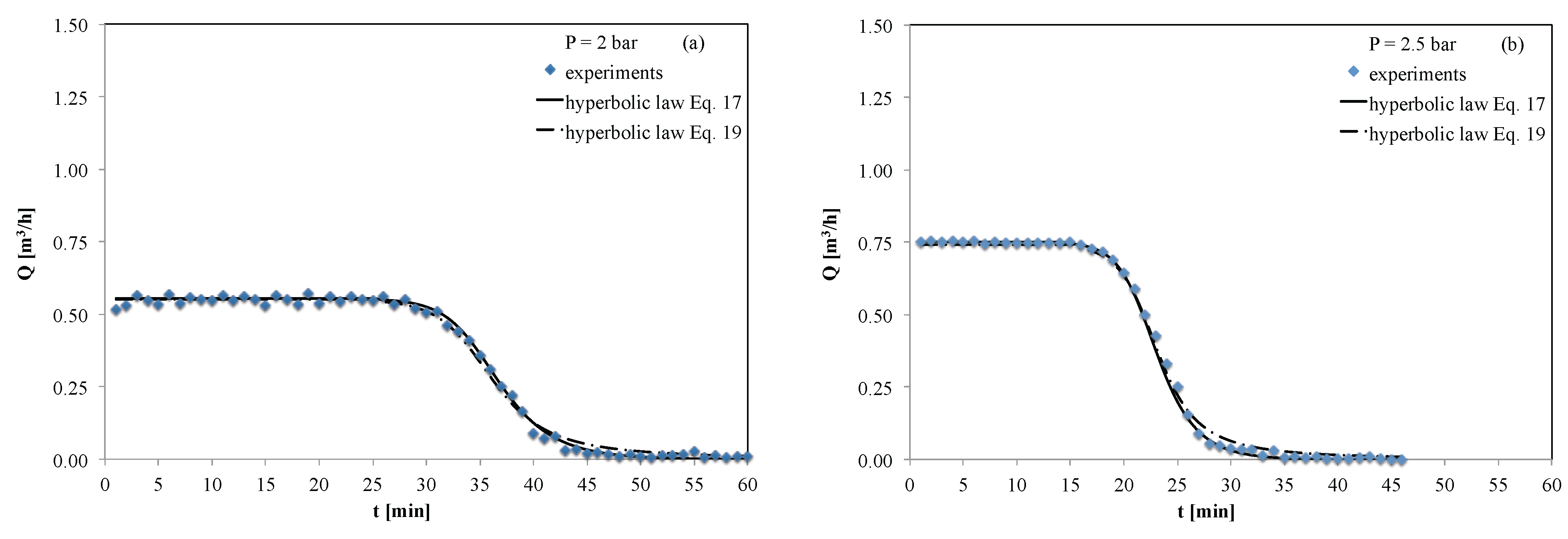
As recently observed by De Marchis et al. [19], although the system of Equations (13) and (14) is able to capture the valve-closing phase, some deviations are observed, particularly at the beginning and at the end of the valve closure. Aiming to reduce the inaccuracy level of the float valve model, a simple mathematical model is proposed here to reproduce the supply system in water tanks. Specifically, a new formulation of the emitter coefficient is proposed, as follows:

$$C_v=f\left(h\right)=\left\{\begin{array}{cc}{C}_v=C_v^{*}\hfill & \text{if }h\le h_{min}\hfill \\ \\ C_v=C_v^{*}·\text{tanh}\left(m·{\displaystyle \frac{h_{max}-h}{h_{max}-h_{min}}}\right)\hfill & \text{if }h>h_{min}\hfill \end{array}\right.$$

(16)

Equation (16) was obtained through the best fit to the laboratory measurements, used to compare the proposed pressure-discharge relationship for demands, when a tank is present. Introducing Equation (16) into Equation (13), it is obtained:

$$\left\{\begin{array}{cc}{Q}_{up}=0\hfill & \text{if }{H}_j\le z_r\hfill \\ \\ Q_{up}=C_v^{*}{a}_v\sqrt{2g(H-z_r)}\hfill & \text{if }h\le h_{min}\hfill \\ \\ Q_{up}=C_v^{*}·\text{tanh}\left(m·{\displaystyle \frac{h_{max}-h}{h_{max}-h_{min}}}\right)a_v\sqrt{2g(H-z_r)}\hfill & \text{if }h>h_{min}\hfill \\ \\ Q_{up}=0\hfill & \text{if }h\ge h_{max}\hfill \end{array}\right.$$

(17)

Following Criminisi et al. [18], the system of Equation (16) was integrated considering a specific equation for the discharge area $a_v$. Similar to Equation (16), a hyperbolic tangent law has been considered:

$$a_v=f\left(h\right)=\left\{\begin{array}{cc}{a}_v=a_v^{*}\hfill & \text{if }h\le h_{min}\hfill \\ \\ a_v=a_v^{*}·\text{tanh}\left(n·{\displaystyle \frac{h_{max}-h}{h_{max}-h_{min}}}\right)\hfill & \text{if }h>h_{min}\hfill \end{array}\right.$$

(18)

The coefficient n of Equation (18) was calibrated through laboratory experiments. Adding Equation (18) into Equation (17), the equation for the flow rate discharging into the water tank reads:

$$\left\{\begin{array}{cc}{Q}_{up}=0\hfill & \text{if }H\le z_r\hfill \\ \\ Q_{up}=C_v^{*}{a}_v^{*}\sqrt{2g(H-z_r)}\hfill & \text{if }h\le h_{min}\hfill \\ \\ Q_{up}=C_v^{*}{a}_v^{*}·\text{tanh}\left(m{\displaystyle \frac{h_{max}-h}{h_{max}-h_{min}}}\right)\text{tanh}\left(n{\displaystyle \frac{h_{max}-h}{h_{max}-h_{min}}}\right)\sqrt{2g(H-z_r)}\hfill & \text{if }h>h_{min}\hfill \\ \\ Q_{up}=0\hfill & \text{if }h\ge h_{max}\hfill \end{array}\right.$$

(19)

4. Experimental Setup

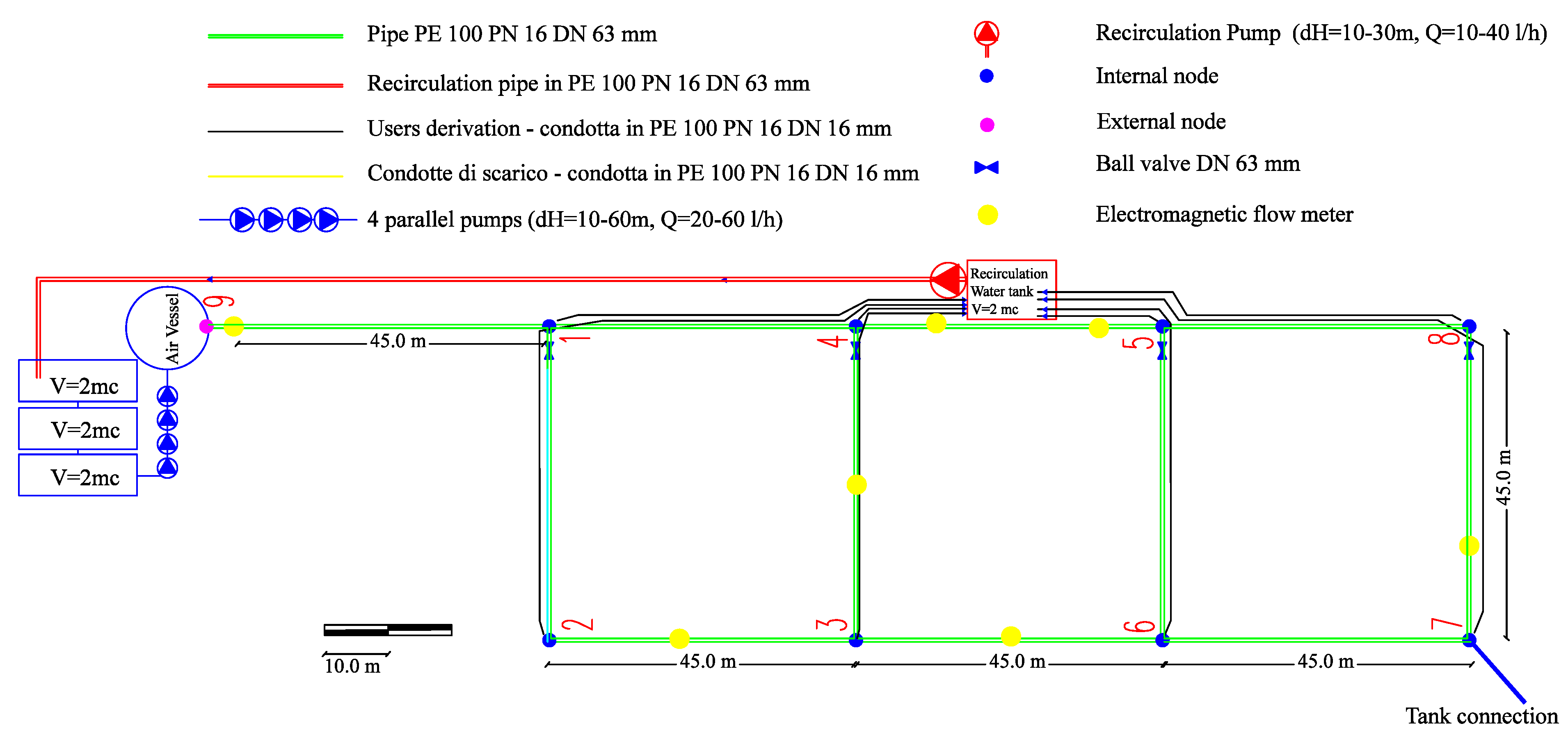
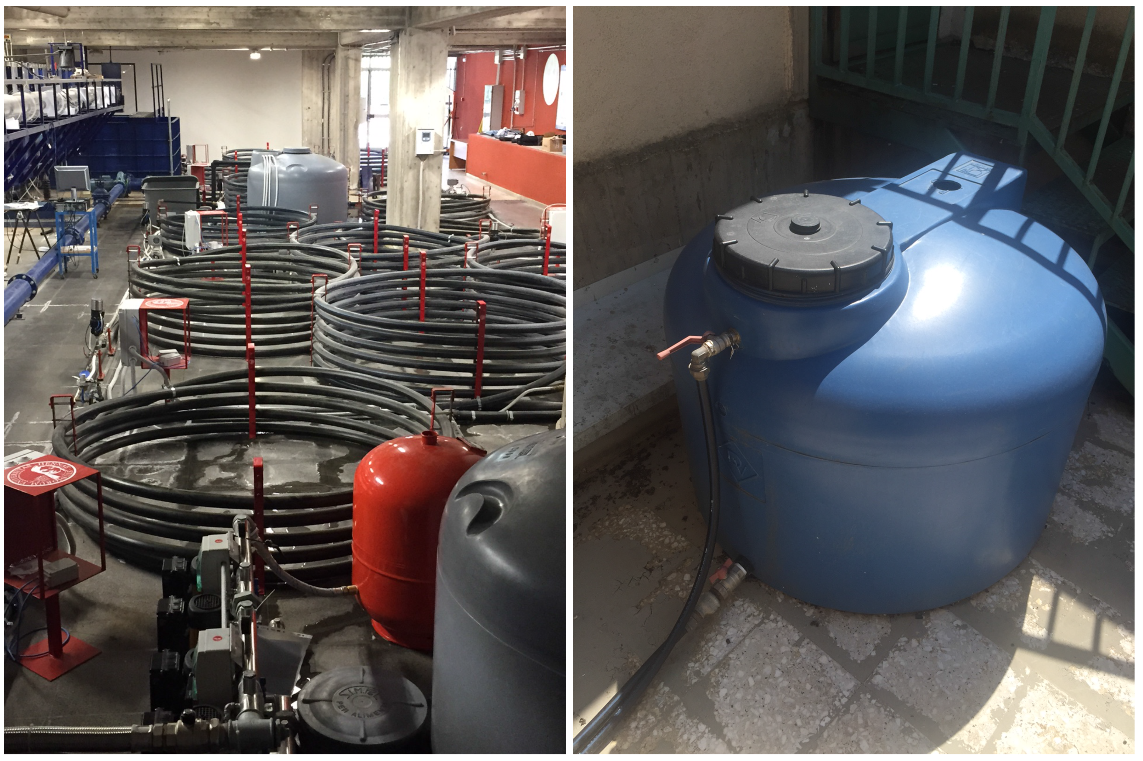
The experiments were conducted at the Environmental Hydraulic Laboratory of the University of Enna (Italy). The flow facility is composed of a water distribution network of high-density polyethylene (HDPE 100 PN16) pipes, designed with three main loops (M = 3), eight internal nodes (N = 8), one external node (S = 1) and eleven pipes (L = 11) with a diameter (DN) of 63 mm. In Figure 1 is plotted a schematic representation of the network. All pipes are enveloped in concentric circles, with a mean diameter of approximately 2 m (as shown in Figure 2a, where a picture of the laboratory is reported), thus achieving a length of approximately 45 m. Four ball valves are located in four different pipes, thereby enabling simulations of networks having one, two or three loops, as well as an inline pipe of approximately 500 m. Figure 1 presents a schematic representation of the water distribution network. The network is fed by four pumps (P), which operate in parallel, connected to three water tanks having a capacity of 2 m${}^3$ each. All of the pumps are equipped with an inverter, thereby enabling changes in the speed rotation and variations in the water head in a range from 10 to 60 m. The system is monitored by 7 electromagnetic flow meters located in Pipes 9–1, 4–5, 3–6, 2–3, 3–6 and 7–8 of the network. Pressure cells and multi-jet water meters are distributed over the entire network at each node position. The network is designed to model the effect of real losses and of apparent losses. The apparent loss are analyzed through a private tank, which is located on the roof of the laboratory at approximately 17.5 m above the network level and is connected to the system through a high-density polyethylene (HDPE 100 PN16) pipe that is 30 m long with a diameter of 12.7 mm. The tank filling process is governed by a float ball valve, BS 1212 type. 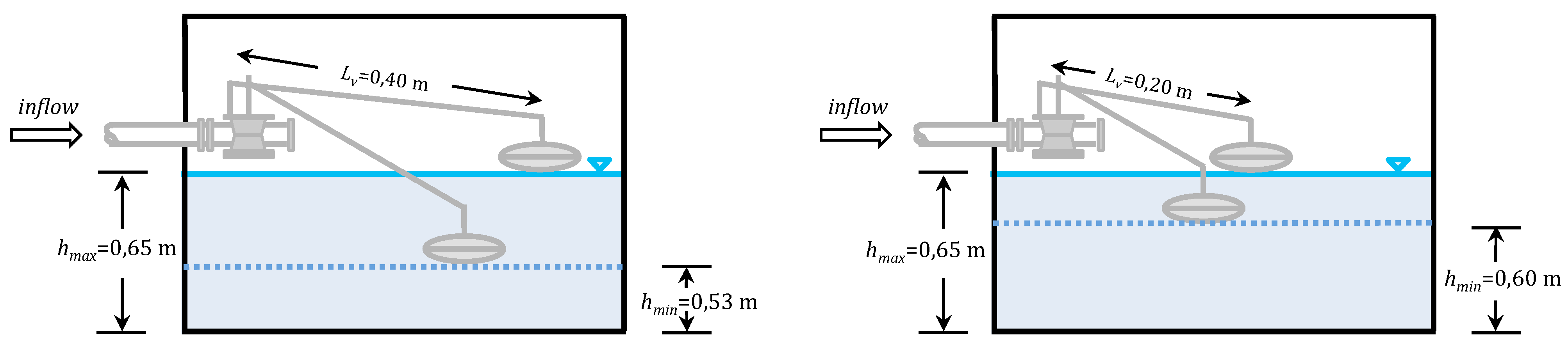Figure 3 presents a schematic of the water tank and float valve. Figure 2 shows a view of the laboratory and of the roof tank. Details on the water distribution system can be found in De Marchis et al. [19].

Figure 1. Layout of the water distribution network.

Figure 1. Layout of the water distribution network.

Experiments

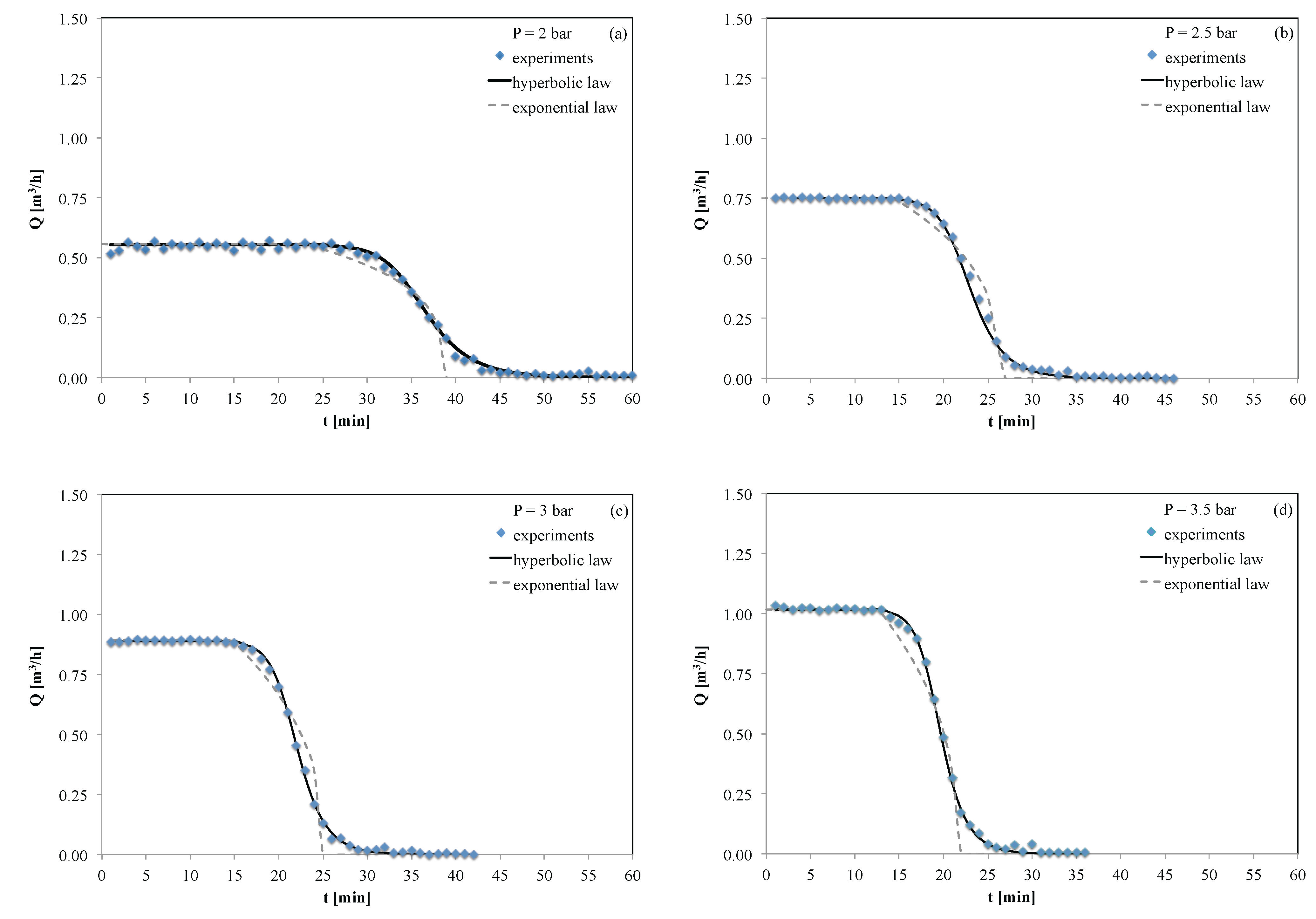
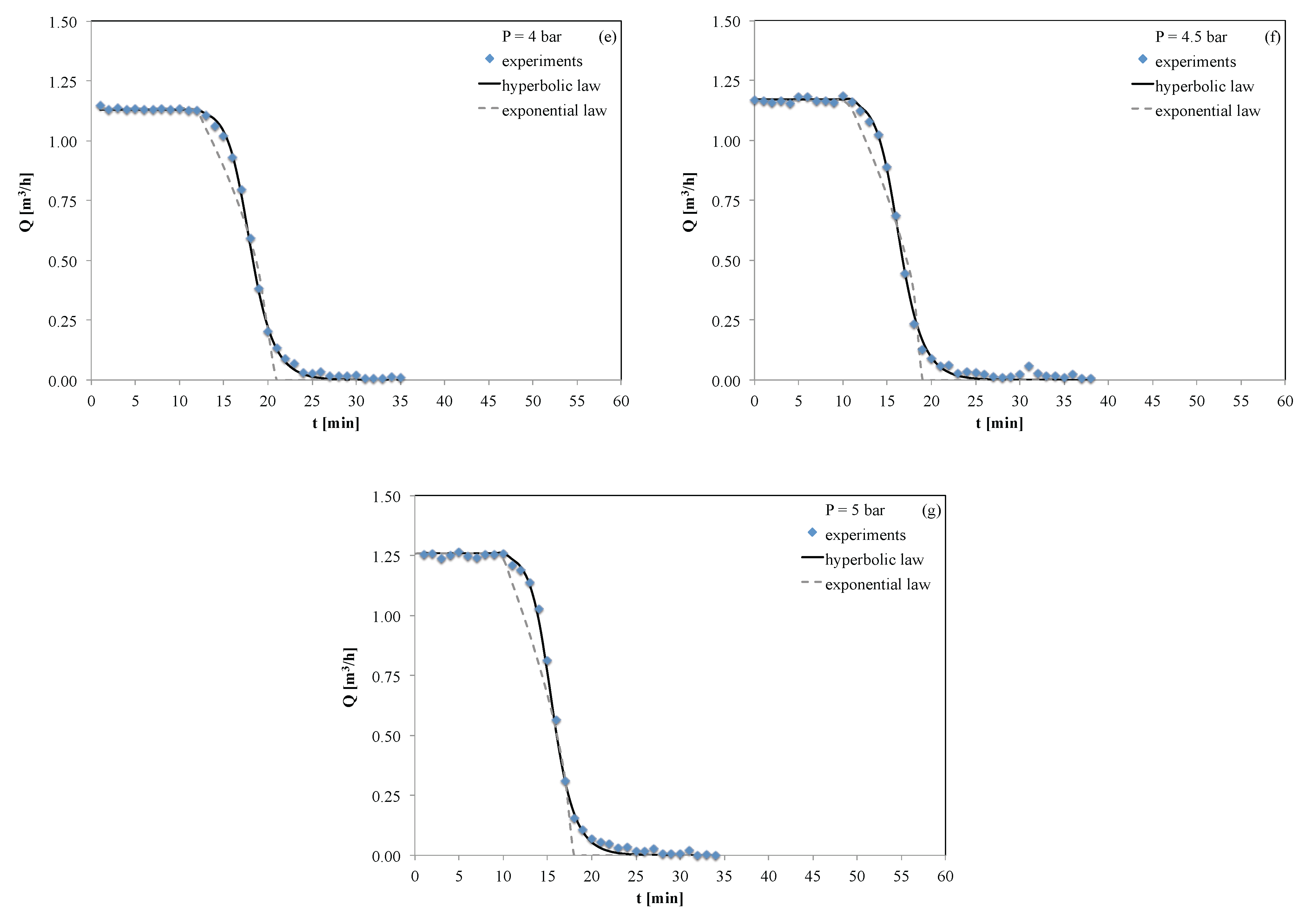
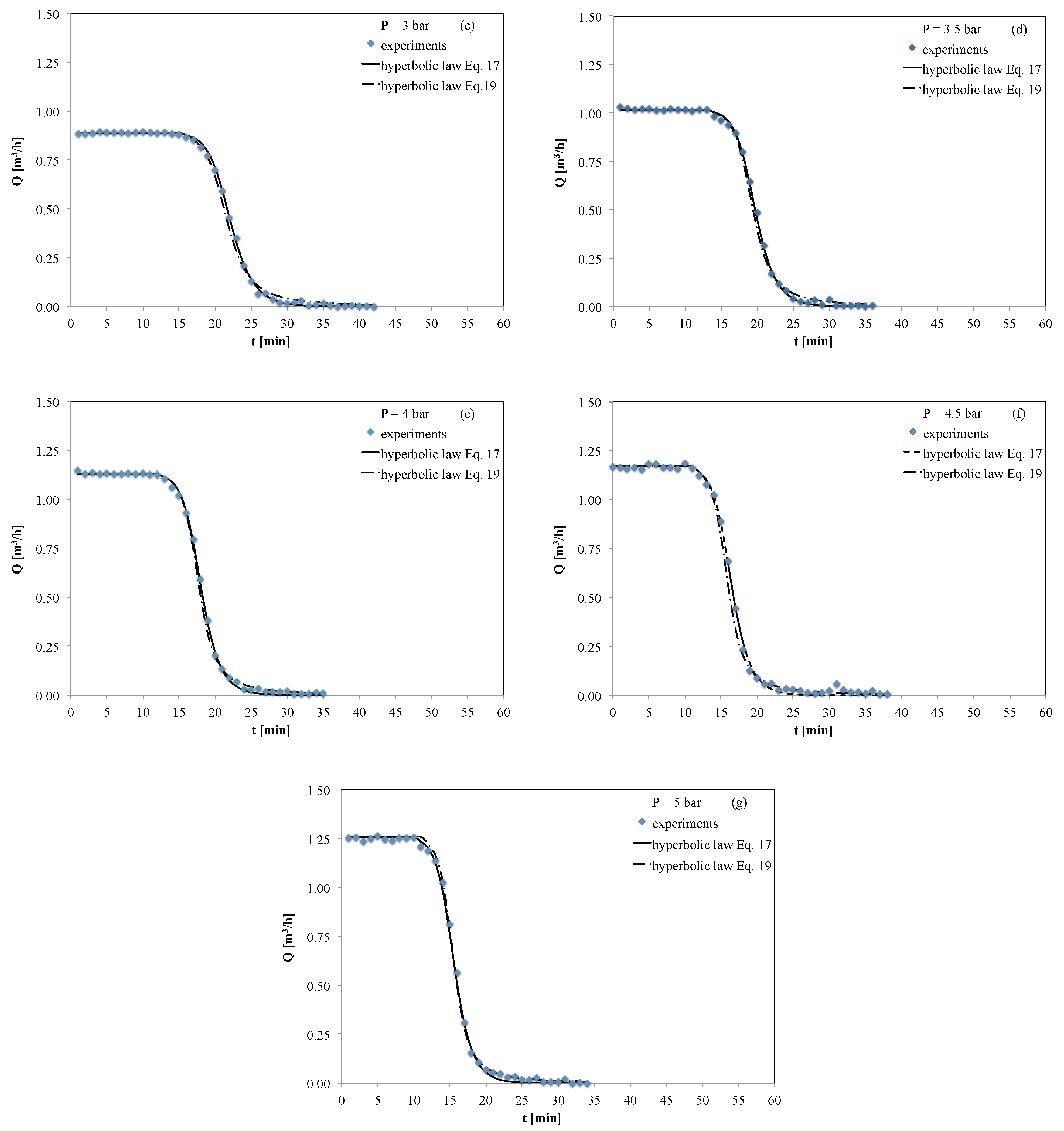
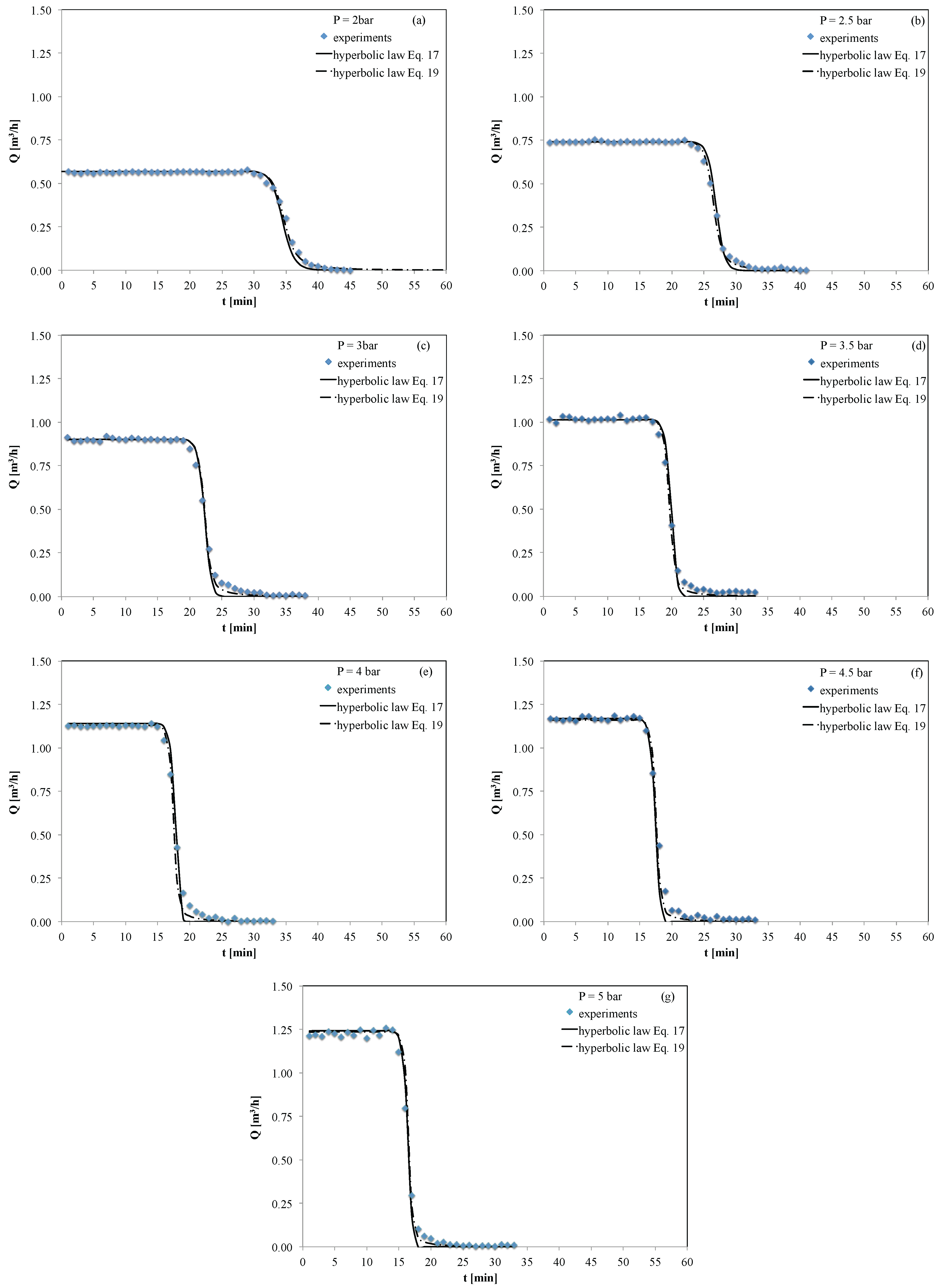
To determine the optimal empirical law to calculate the flow discharging into the local reservoir, two set of experiments were conducted in which the length of the float valve branch was modified. Specifically, in the first set of simulations, a branch with a length of approximately 40 cm was installed (Test Case 1 (TC1)), whereas in the second set of experiments, the float valve was equipped with a branch of approximately 20 cm (TC2); see Figure 3. In the first test case, the float valve starts to close when the water level inside the tank reaches a depth of $h_{min}$ = 0.53 cm, whereas when the water depth is $h_{max}$ = 0.65 cm, the valve can be considered completely closed. In contrast, in TC2, $h_{min}$ = 0.60 cm. In all cases, the experiments were performed considering that at the beginning of each test, the water tank was empty, and then, the tank is filled considering the daily water supply of the user (350 L per inhabitant per day); this condition simulates a daily intermittent network in which the tank is filled every two days, and it is emptied on the day in which water supply is not guaranteed (see [15,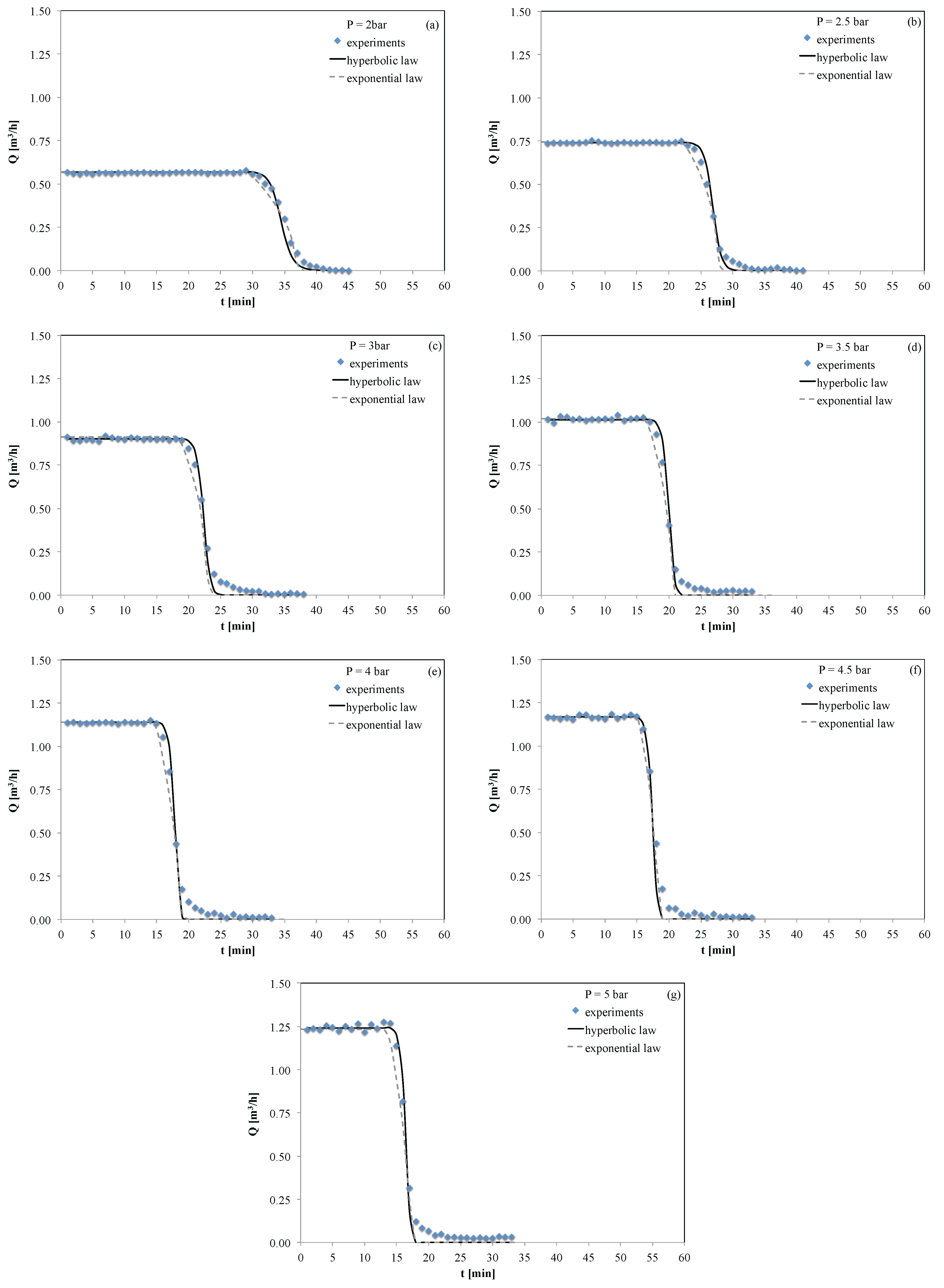26]). For each test case, four scenarios were simulated by changing the pressure from 2 bar to 5 bar, with a step of 0.5 bar. The water volume flowing into the tank was estimated using the electromagnetic flow meter of the ABB IM/WM type (with an accuracy of 0.4%) installed in the inlet pipe, downstream of the pump station. The hydraulic head H used in Equation (13) to estimate $Q_{up}$ was measured using a piezoresistive pressure transducer Gems sensor 3100 series (with an accuracy of 0.1%) located in Node 7. The data were collected using a sampling rate of 1 Hz. Each experiment was repeated twice, and the average value was considered. The experiments were used to calibrate the empirical law proposed in the present study.

Figure 2. Layout of the water distribution network and view of the roof tank.

Figure 2. Layout of the water distribution network and view of the roof tank.

Figure 3. Layout of the water tank and the float valve. Left: short branch; right: long branch.

Figure 3. Layout of the water tank and the float valve. Left: short branch; right: long branch.

5. Results

The proposed mathematical model is able to reproduce the flow discharging into a local tank. The discharge is controlled by a float valve calibrated on the basis of experimental data. Initially, the experimental data were compared to the exponential law proposed by Criminisi et al. [18] (Equation (14)) and to the proposed hyperbolic tangent law (Equation (16)), suggested here, considering the discharge area $a_v$ as being constant. At a later stage, the analytical results from the hyperbolic tangent law, obtained considering a constant discharge area $a_v$ = cost, were compared to the results achieved from the system of Equations (16) and (18), thus considering the effective reduction of the float valve area.

5.1. Comparison between Experiments and Mathematical Laws, Considering a Constant Discharge Area $a_v$

Figure 4 compares data collected from the TC1 tests with results obtained from the analytical law proposed by Criminisi et al. [18] and from the hyperbolic law proposed in this work. Experiments were performed for different pressure values in the range between two and five bar, with a step of 0.5 bar. In the present analysis, the lowest value of pressure, equal to two bar, was chosen considering that the water tank is located on the roof of the laboratory at approximately 17.5 m above the pump station, where the two bar is measured. In this way, it was possible to analyze also low pressures, typical of the head-driven models. Overall, as expected, the more the hydraulic head increases, the more the flow rate Q increases. The filling process becomes increasingly shorter, and the front of the curve, which is representative of the closure phase of the valve, progressively increases its slope, consistent with a more rapid closure of the valve. From Figure 4a, it can be observed that the filling process is completed in 60 min, collecting approximately 350 L. The same amount of water volume is stored in approximately 35 min when the water head pressure is five bar (see Figure 4g). The comparison between the experimental data and hyperbolic laws clearly shows that although both equations are able to capture the experimental results, the line representative of Equation (16) perfectly reproduces the filling process. Equations (14) and (16) clearly overlap each other until $h<h_{min}$. When $h>h_{min}$, the exponential law exhibits deviations from the measured data, whereas the proposed hyperbolic tangent law perfectly reproduces the experimental flow rate during the entire filling process. The collected data reported in Figure 4 have been averaged to achieve one data point per minute.

The obtained results demonstrate the ability of the proposed model to estimate the flow discharging into a private tank when the discharge is governed by a float valve. The hyperbolic tangent law can be thus used in numerical codes to improve the node demand models in cases characteristic of Mediterranean countries, where users address water scarcity conditions through the use of local reservoirs.

Figure 4. Test Case 1. Flow rate during the tank filling process, considering a constant value of $a_v$. ⧫: experiments; bold line: hyperbolic law; dashed line: exponential law. (a) Pressure two bar; (b) pressure 2.5 bar; (c) pressure three bar; (d) pressure 3.5 bar; (e) pressure four bar; (f) pressure 4.5 bar; (g) pressure five bar.

Figure 4. Test Case 1. Flow rate during the tank filling process, considering a constant value of $a_v$. ⧫: experiments; bold line: hyperbolic law; dashed line: exponential law. (a) Pressure two bar; (b) pressure 2.5 bar; (c) pressure three bar; (d) pressure 3.5 bar; (e) pressure four bar; (f) pressure 4.5 bar; (g) pressure five bar.

To verify the effectiveness of the proposed hyperbolic tangent law, the mathematical model was compared to a second set of laboratory experiments, previously indicated as TC2. Figure 5 plots the flow rate data collected using a short branch adopting the same pressure conditions used for the TC1 experimental sets. The TC1 and TC2 experimental setups are characterized by two different values of the valve branch: 0.40 m for the TC1 setup and 0.20 m for the TC2 setup. As long as the water inside the tank is lower than $h_{min}$, the TC2 experimental data overlap with the TC1 results, whereas for $h>h_{min}$, the valve closure is clearly more rapid than that observed in TC1. Once again, Criminisi et al. [18] and the proposed hyperbolic law reproduce the experimental data well. Even though the exponential law seems to reproduce the collected data, also in this case, the hyperbolic law, given by Equation (16), shows a better agreement than Equation (14). Comparing the fitting of the hyperbolic tangent law shown in Figure 4 and Figure 5, it can be observed that a worse agreement is verified for TC2. This is necessary for obtaining a universal law for the coefficient m. In fact, as shown in Figure 6, the values of the coefficient m are clearly aligned for both the TC1 and TC2 experimental series of data. Finally, to predict the flow rate $Q_{up}$, the Torricelli law, Equation (13) and the emitter coefficient equation, Equation (16), must be completed using the linear dependence of m with the water head through the equation:

$$m=-0.018H+3.35$$

(20)

Figure 5. Test Case 2. Flow rate during the tank filling process, considering a constant value of $a_v$. ⧫: experiments; bold line: hyperbolic law; dashed line: exponential law. (a) Pressure two bar; (b) pressure 2.5 bar; (c) pressure three bar; (d) pressure 3.5 bar; (e) pressure four bar; (f) pressure 4.5 bar; (g) pressure five bar.

Figure 5. Test Case 2. Flow rate during the tank filling process, considering a constant value of $a_v$. ⧫: experiments; bold line: hyperbolic law; dashed line: exponential law. (a) Pressure two bar; (b) pressure 2.5 bar; (c) pressure three bar; (d) pressure 3.5 bar; (e) pressure four bar; (f) pressure 4.5 bar; (g) pressure five bar.

Figure 6. Variation of the coefficient m with the pressure (P). ⧫: Test Case 1; •: Test Case 2; thin line: interpolation curve. (a) Hyperbolic tangential law. Thin line equation: m = −0.018H + 3.35; (b) exponential law. Thin line equation: m = 0.0027H + 0.23 [19].

Figure 6. Variation of the coefficient m with the pressure (P). ⧫: Test Case 1; •: Test Case 2; thin line: interpolation curve. (a) Hyperbolic tangential law. Thin line equation: m = −0.018H + 3.35; (b) exponential law. Thin line equation: m = 0.0027H + 0.23 [19].

The emitter parameter $C_v^{*}$ of the open valve, plotted in Figure 7 decreases with pressure depending on the increase in local head loss due to the valve, and, as reported in the preliminary research of De Marchis et al. [19], the variation is not linear; in the analyzed case, it is well interpolated by the following power law:

$$C_v^{*}=C_{v0}+d·{(P-P_0)}^{-k}$$

(21)

where $C_{v0}$ is a horizontal asymptote equal to 0.276, $P_0$ is a vertical asymptote equal to 11.1 and b and n are shape coefficients calibrated to 6.24 and 1.27, respectively.

Figure 7. Variation of the emitter coefficient $C_v^{*}$ with P. •: Test Case 1; ⧫: Test Case 2; bold line: interpolation law: $C_v^{*}$ = $C_{v0}+d·{(P-P_0)}^{-k}$.

Figure 7. Variation of the emitter coefficient $C_v^{*}$ with P. •: Test Case 1; ⧫: Test Case 2; bold line: interpolation law: $C_v^{*}$ = $C_{v0}+d·{(P-P_0)}^{-k}$.

5.2. Comparison between Experiments and Mathematical Laws, Considering a Variable Discharge Area $a_v$

Although the above results demonstrate the ability of the proposed numerical model to capture a fast closure of the float valve, some deviations were observed when the valve closure is nearly complete, at least for the short branch. To improve the model, a hyperbolic tangent law for the discharge area $a_v$ was considered, through Equation (18). Figure 8 and Figure 9 show comparisons between the experimental data and the proposed mathematical laws, Equations (17) and (19) for the TC1 and TC2 experimental setups, respectively. Figure 8 shows that for the TC1 results, both of the mathematical laws show a good agreement and overlap each other with no substantial differences. This result confirms that both of the laws can be considered valid tools for modeling the inline tank filling process. On the other hand, in Figure 9, it can be observed that when the hyperbolic tangent law is used for the discharge area $a_v$, a better agreement with the experiments is achieved, particularly at the final part of the closing phase. Hence, it can be concluded that when a hyperbolic tangent law is used for both coefficients $C_v$ and $a_v$, the model is able to perfectly reproduce the supply system in WDNs that are characterized by the presence of private tanks installed by users. Note that both Equations (17) and (19) have the same computational cost when implemented in the numerical model. Regardless, the primary goal of Equation (19) is that the coefficients m and n have a constant value for all pressures and for both of the valve branches. Specifically, the results presented in Figure 8 and Figure 9, achieved through Equation (19), have been obtained by assigning m=2.5 and n=4. Interestingly, when the hyperbolic tangent law governs the discharge area $a_v$ variation, a slight improvement in the performance of the model is observed, and Equation (20), which is representative of the linear variation of the coefficient m, must not be considered, thereby reducing the number of equations to resolve in numerical models. This is an important result, particularly when it is necessary to solve WDNs possessing many supply nodes.

Table 1 collects the values of the coefficients $C_v^{*}$, m and n achieved by fitting the experimental data for both the exponential and hyperbolic laws. As expected, the coefficient $C_v^{*}$ has the same values independent of the float valve. In contrast, the coefficients m and n are strictly affected by the law of the discharge, e.g., exponential or hyperbolic. However, note that when the discharge into the tank is calculated using a hyperbolic law, both for the emitter coefficient and for the discharge area, the coefficients m and n achieve a constant value for all types of branches and for the entire pressure interval considered.

Table 1. Coefficients of the float valve laws achieved for the experimental law and for the proposed hyperbolic laws. TCI, Test Case 1.

Test Case	Equation	Coefficient	2 bar	2.5 bar	3 bar	3.5 bar	4 bar	4.5 bar	5 bar
TC1	Equation (14)	m	0.30	0.30	0.32	0.33	0.35	0.37	0.38
TC2	Equation (14)	m	0.29	0.30	0.30	0.32	0.33	0.35	0.37
TC1	Equation (17)	m	2.94	2.88	2.80	2.67	2.57	2.49	2.42
TC2	Equation (17)	m	2.95	2.87	2.76	2.68	2.57	2.50	2.40
All cases	Equation (19)	m	2.50	2.50	2.50	2.50	2.50	2.50	2.50
All cases	Equation (19)	n	4.00	4.00	4.00	4.00	4.00	4.00	4.00
TC1	Equation (21)	$C_v^{*}$	0.61	0.43	0.39	0.37	0.36	0.35	0.33
TC2	Equation (21)	$C_v^{*}$	0.62	0.45	0.39	0.38	0.37	0.36	0.35

Table 1. Coefficients of the float valve laws achieved for the experimental law and for the proposed hyperbolic laws. TCI, Test Case 1.

Test Case	Equation	Coefficient	2 bar	2.5 bar	3 bar	3.5 bar	4 bar	4.5 bar	5 bar
TC1	Equation (14)	m	0.30	0.30	0.32	0.33	0.35	0.37	0.38
TC2	Equation (14)	m	0.29	0.30	0.30	0.32	0.33	0.35	0.37
TC1	Equation (17)	m	2.94	2.88	2.80	2.67	2.57	2.49	2.42
TC2	Equation (17)	m	2.95	2.87	2.76	2.68	2.57	2.50	2.40
All cases	Equation (19)	m	2.50	2.50	2.50	2.50	2.50	2.50	2.50
All cases	Equation (19)	n	4.00	4.00	4.00	4.00	4.00	4.00	4.00
TC1	Equation (21)	$C_v^{*}$	0.61	0.43	0.39	0.37	0.36	0.35	0.33
TC2	Equation (21)	$C_v^{*}$	0.62	0.45	0.39	0.38	0.37	0.36	0.35

Figure 8. Test Case 1. Comparison between the flow rate during the tank filling process obtained considering a constant value of $a_v$ and a hyperbolic law for $a_v$. ⧫: experiments; dashed line: Equation (17); bold line: Equation (19). (a) Pressure 2 bar; (b) pressure 2.5 bar; (c) pressure three bar; (d) pressure 3.5 bar; (e) pressure four bar; (f) pressure 4.5 bar; (g) pressure five bar.

Figure 8. Test Case 1. Comparison between the flow rate during the tank filling process obtained considering a constant value of $a_v$ and a hyperbolic law for $a_v$. ⧫: experiments; dashed line: Equation (17); bold line: Equation (19). (a) Pressure 2 bar; (b) pressure 2.5 bar; (c) pressure three bar; (d) pressure 3.5 bar; (e) pressure four bar; (f) pressure 4.5 bar; (g) pressure five bar.

Figure 9. Test Case 2. Comparison between the flow rate during the tank filling process obtained considering a constant value of $a_v$ and a hyperbolic law for $a_v$. ⧫: experiments; dashed line: Equation (17); bold line: Equation (19). (a) Pressure two bar; (b) pressure 2.5 bar; (c) pressure three bar; (d) pressure 3.5 bar; (e) pressure four bar; (f) pressure 4.5 bar; (g) pressure five bar.

Figure 9. Test Case 2. Comparison between the flow rate during the tank filling process obtained considering a constant value of $a_v$ and a hyperbolic law for $a_v$. ⧫: experiments; dashed line: Equation (17); bold line: Equation (19). (a) Pressure two bar; (b) pressure 2.5 bar; (c) pressure three bar; (d) pressure 3.5 bar; (e) pressure four bar; (f) pressure 4.5 bar; (g) pressure five bar.

6. Conclusions

In this study, the pressure-discharge relations used to calculate the flow rate in inline private tanks have been analyzed. In several countries, water distribution networks are directly connected to local reservoirs, which are used by users to collect water during periods of water scarcity conditions. Private water tanks greatly affect the hydraulic behavior of the network, modifying users’ demand patterns. To help mathematical models correctly simulate this demand configuration while taking into account these specific installations, a new mathematical formulation has been proposed and validated against experimental data. The analysis has been performed considering a wide range of experimental head pressures. A new pressure-discharge relation has been proposed, which is more reliable than some previous relationships proposed in the literature. A hyperbolic tangent law is proposed for the emitter coefficient $C_v$ of the head-discharge relationship and for the discharge area $a_v$ of the float valve. The mathematical model has been compared to existing float valve laws and to laboratory experiments, which were performed considering seven different pressure values in two branches characterized by different lengths. The results demonstrate the ability of the proposed hyperbolic tangent law to reproduce the filling process, both when the valve is completely open and during the valve closure period. The mathematical system obtained can be used in the steady state and in the transient model, and it is able to correctly estimate the supplied demand when private tanks equipped with float valves are installed in the network.

References

1. Tabesh, M.; Shirzad, A.; Arefkhani, V.; Mani, A. A comparative study between the modified and available demand driven based models for head driven analysis of water distribution networks. Urban Water J. 2014, 11, 221–230. [Google Scholar] [CrossRef]
2. Chandapillai, J. Realistic simulation of water distribution system. J. Transp. Eng. 1991, 117, 258–263. [Google Scholar] [CrossRef]
3. Puleo, V.; Fontanazza, M.C.; Notaro, V.; de Marchis, M.; Freni, G.; la Loggia, G. Pumps as turbines (PATs) in water distribution networks affected by intermittent service. J. Hydroinform. 2014, 16, 259–271. [Google Scholar] [CrossRef]
4. Bhave, P.R. Node flow analysis of water distribution systems. J. Transp. Eng. 1981, 107, 457–467. [Google Scholar]
5. Tabesh, M.; Tanyimboh, T.T.; Burrows, R. Head driven simulation of water supply networks. Eng. Trans. A Basics 2001, 15, 11–22. [Google Scholar]
6. Germanopoulos, G. A technical note on the inclusion of pressure dependent demand and leakage terms in water supply network models. Civil Eng. Syst. 1985, 2, 171–179. [Google Scholar] [CrossRef]
7. Wagner, J.M.; Shamir, U.; Marks, D.H. Water distribution reliability: Simulation methods. J. Water Res. Plan. Manag. 1988, 114, 276–294. [Google Scholar] [CrossRef]
8. Reddy, L.S.; Elango, K. Analysis of water distribution networks with head dependent outlets. Civil Eng. Syst. 1989, 6, 102–110. [Google Scholar] [CrossRef]
9. Jowitt, P.W.; Xu, C. Predicting pipe failure effects in water distribution networks. J. Water Res. Plan. Manag. 1993, 119, 18–31. [Google Scholar] [CrossRef]
10. Gupta, R.; Bhave, P.R. Comparison of methods for predicting deficient-network performance. J. Water Res. Plan. Manag. 1996, 122, 214–217. [Google Scholar] [CrossRef]
11. Tucciarelli, T.; Criminisi, A.; Termini, D. Leak analysis in pipeline systems by means of optimal valve regulation. J. Hydraul. Eng. 1999, 125, 277–285. [Google Scholar] [CrossRef]
12. Ackley, J.R.L.; Tanyimboh, T.T.; Tahar, B.; Templeman, A.B. Head-driven analysis of water distribution systems. In Computer and Control in Water Industry, Water Software Systems: Theory and Applications; Ulanicki, B., Ed.; Research Studies Press: Baldock, Hertfordshire, UK, 2001; pp. 183–192. [Google Scholar]
13. Tanyimboh, T.T.; Tabesh, M.; Burrows, R. Appraisal of source head methods for calculating reliability of water distribution networks. J. Water Res. Plan. Manag. 2001, 127, 206–213. [Google Scholar] [CrossRef]
14. Tanyimboh, T.T.; Templeman, A.B. A new nodal outflow function for water distribution networks. In Proceedings of the 4th International Conference on Engineering Computational Technology (CD-ROM), Lisbon, Portugal, 7–9 September 2004; Civil-Comp Press: Stirling, UK, 2004; p. 64. [Google Scholar]
15. De Marchis, M.; Fontanazza, C.M.; Freni, G.; la Loggia, G.; Napoli, E.; Notaro, V. A model of the filling process of an intermittent distribution network. Urban Water J. 2010, 7, 321–333. [Google Scholar] [CrossRef]
16. Freni, G.; de Marchis, M.; Napoli, E. Implementation of pressure reduction valves in a dynamic water distribution numerical model to control the inequality in water supply. J. Hydroinform. 2014, 16, 207–217. [Google Scholar] [CrossRef] [Green Version]
17. Giustolisi, O.; Berardi, L.; Laucelli, D. Modeling Local Water Storages Delivering Customer Demands in WDN Models. J. Hydraul. Eng. 2014, 140, 89–104. [Google Scholar] [CrossRef]
18. Criminisi, A.; Fontanazza, C.M.; Freni, G.; la Loggia, G. Evaluation of the apparent losses caused by water meter under-registration in intermittent water supply. Water Sci. Technol. 2009, 60, 2373–2382. [Google Scholar] [CrossRef] [PubMed]
19. De Marchis, M.; Fontanazza, C.M.; Freni, G.; Milici, B.; Puleo, V. Experimental investigation for local tank inflow model. Procedia Eng. 2014, 89, 656–663. [Google Scholar] [CrossRef]
20. Shirzad, A.; Tabesh, M.; Farmani, R.; Mohammadi, M. Pressure-Discharge Relations with Application to Head-Driven Simulation of Water Distribution Networks. J. Water Resour. Plan. Manag. 2013, 139, 660–670. [Google Scholar] [CrossRef]
21. Fujiwara, O.; Ganesharajah, T. Reliability assessment of water supply systems with storage and distribution networks. Water Resour. Res. 1993, 29, 2917–2924. [Google Scholar] [CrossRef]
22. Tabesh, M.; Tanyimboh, T.T. Discussion of comparison of methods for predicting deficient network performance. J. Water Res. Plan. Manag. 1997, 123, 369–370. [Google Scholar]
23. Tabesh, M. Implications of the Pressure Dependency of Outflows on Data Management, Mathematical Modeling and Reliability Assessment of Water Distribution Systems. Ph.D. Thesis, Liverpool University, Liverpool, UK, 1998. [Google Scholar]
24. Tanyimboh, T.T.; Templeman, A.B. Seamless pressure deficient water distribution system model. Water Manag. 2010, 163, 389–396. [Google Scholar] [CrossRef] [Green Version]
25. Wu, Z.Y.; Wang, P.H.; Walski, T.M.; Yang, S.Y.; Bowdler, D.; Baggett, C.C. Extended global-gradient algorithm for pressure-dependent water distribution analysis. J. Water Res. Plan. Manag. 2009, 135, 13–22. [Google Scholar] [CrossRef]
26. De Marchis, M.; Fontanazza, C.M.; Freni, G.; la Loggia, G.; Napoli, E.; Notaro, V. Analysis of the impact of intermittent distribution by modeling the network-filling process. J. Hydroinform. 2011, 13, 358–373. [Google Scholar] [CrossRef]