Simulating Flash Floods at Hourly Time-Step Using the SWAT Model

 ,
,  , ,
, , 
Abstract
1. Introduction
2. Materials and Methods
2.1. Study Design
2.2. Hydrological Models Description
2.2.1. The SWAT Model
2.2.2. The MARINE Model
2.3. Study Area, Selected Flood Events and Input Data
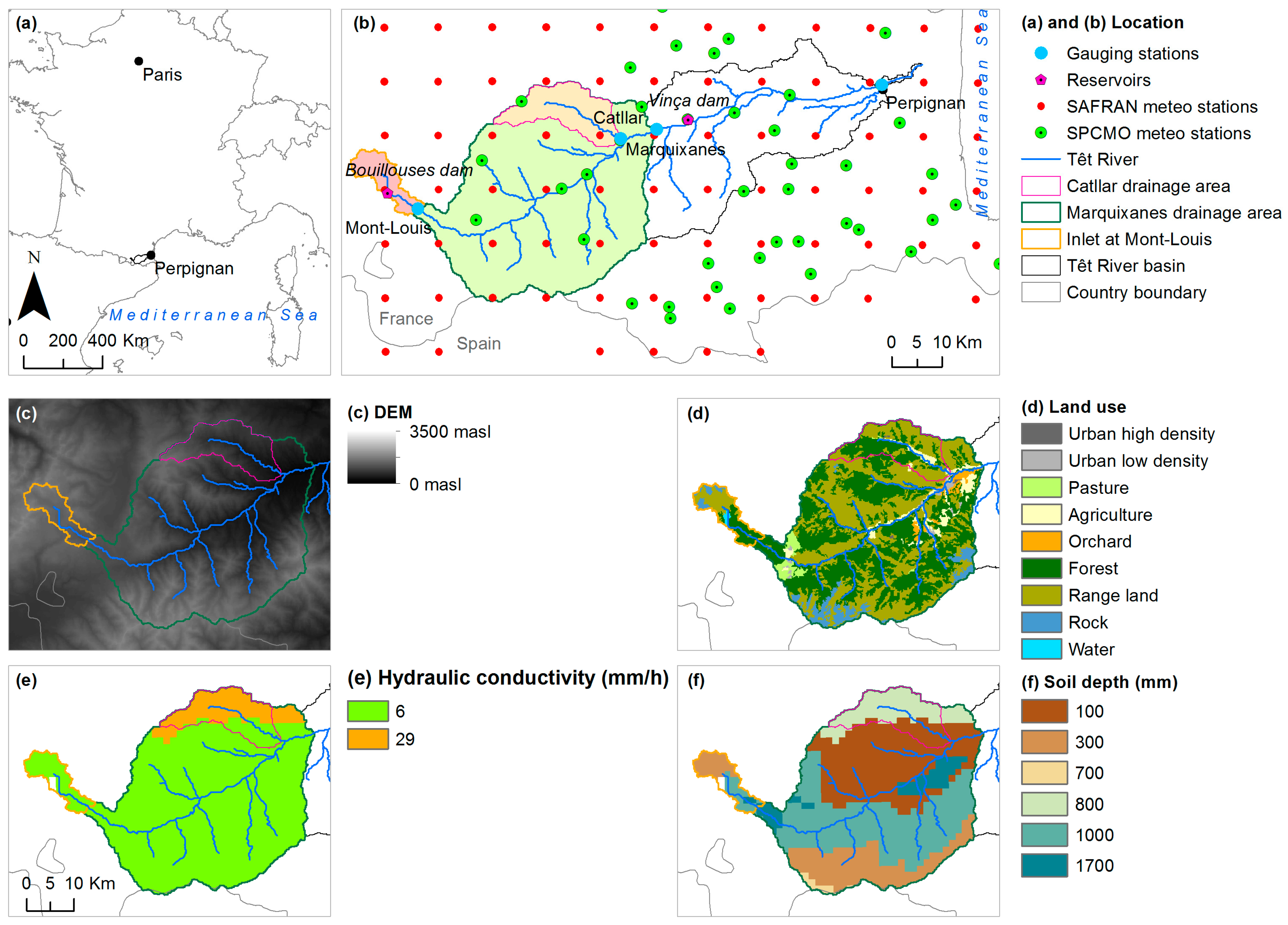
2.3.1. The Têt Watershed
2.3.2. Selected Flash Flood Events
2.3.3. Data Selection for Models’ Set up and Comparison
- Topography was described for both models with the SRTM 90 m digital elevation model [51]
- Land use maps were derived for both models from the 100 m 2006 Corine Land Cover map (Source: European Environmental Agency)
- A common map of soil depth and soil texture was computed based on the Food and Agriculture Organization (FAO) Digital Soil Map of the World (Source: Land and Water Development Division, FAO, Rome), with associated soil properties from the French National Institute of Agronomic Research (INRA). MARINE assumes homogeneous soil profiles and estimates soil classes according to pedotransfer function [52], each soil class being associated to saturated water content, suction and saturated hydraulic conductivity.
2.4. Sensitivity Analysis and Model Calibration and Validation
2.4.1. Procedure for the SWAT Model
- Model delineated with 15 km2 minimum drainage area and simulation at a daily time-step
- Model delineated with 15 km2 minimum drainage area and simulation at an hourly time-step
- Model delineated with 1 km2 minimum drainage area and simulation at an hourly time-step
2.4.2. Procedure for the MARINE Model
3. Results and Discussion
3.1. Time-Continuous Discharge Simulation with SWAT
3.1.1. Parameters’ Sensitivity and Calibration
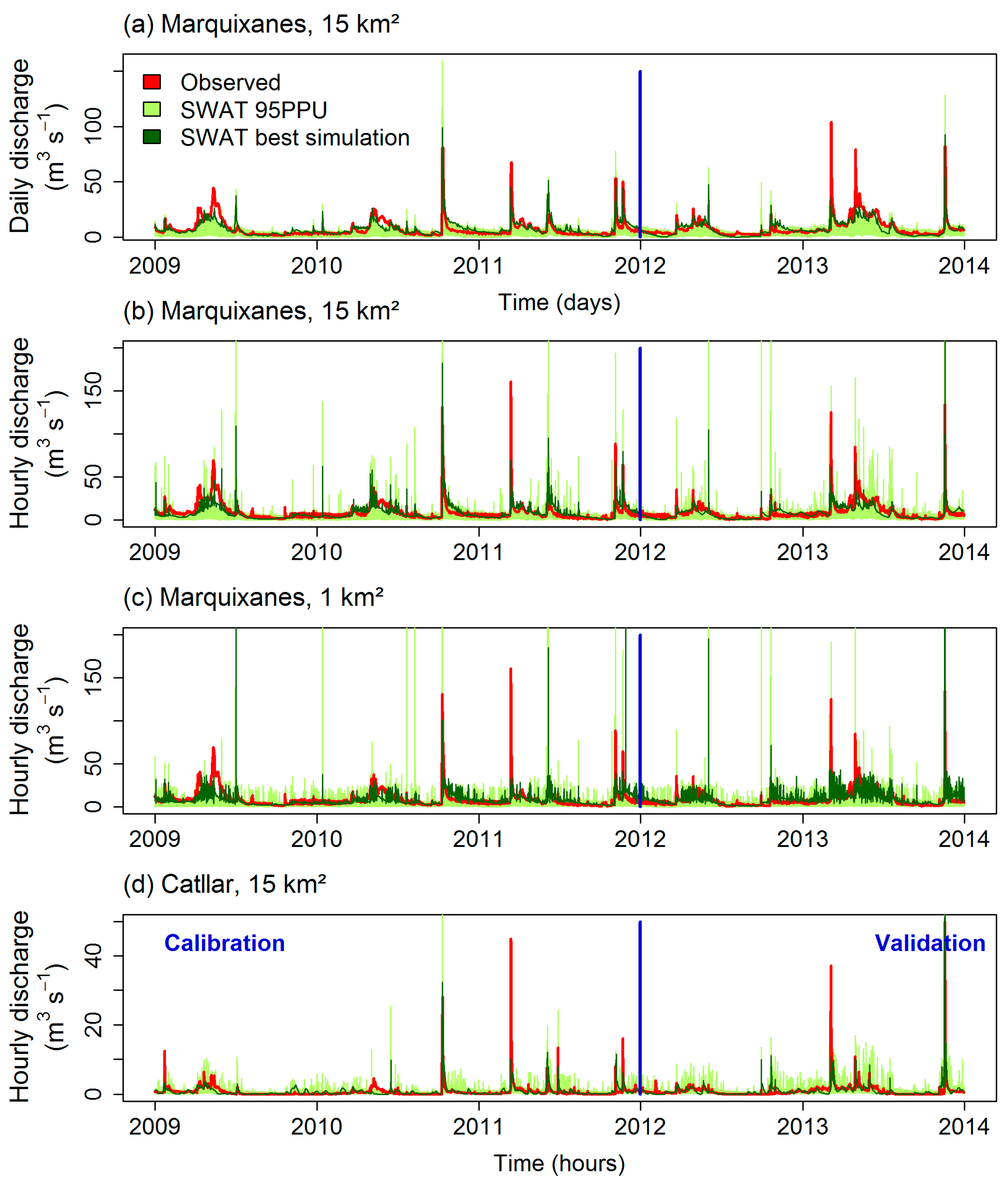
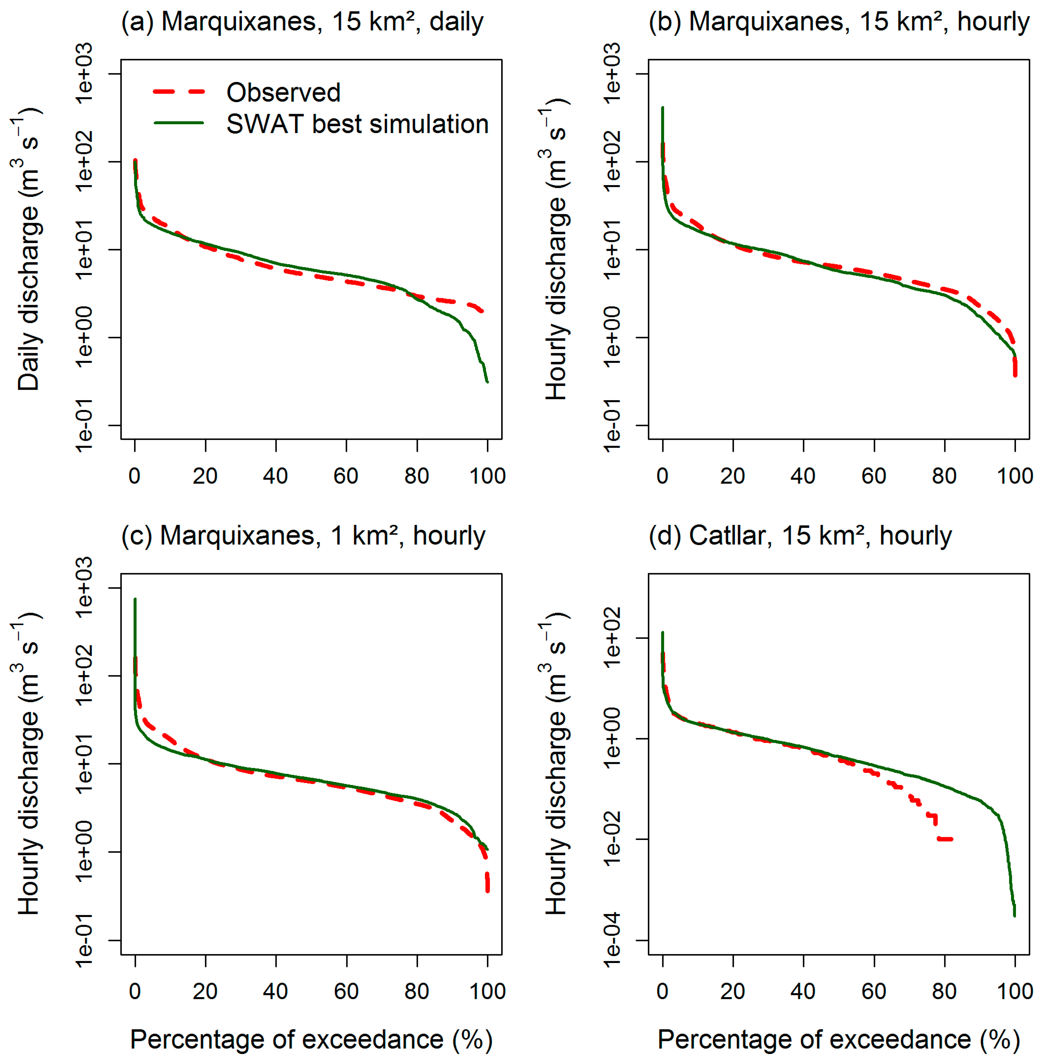
3.1.2. Discharge Calibration and Validation Results in the Main Channel
3.2. Event-Scale Discharge Simulation with MARINE
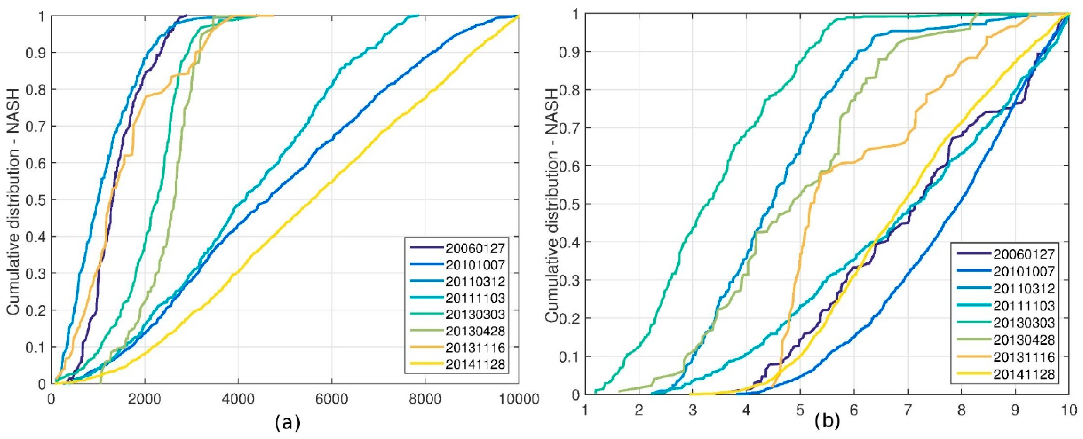
3.2.1. Parameters’ Sensitivity and Calibration
- Most of the behavioral simulations were for CZ values greater than 7 and CKSS values greater than 5000 for the autumn events (20101007, 20111103, 20141128). Most of the behavioral simulations were for CZ values smaller than 5 and CKSS values smaller than 3000 for the spring events (20110312, 20130303, 20130428);
- Two events exhibited different behavior: 20131116 and 20060127. The autumn event 20131116 presented a PDF of CZ that flattened in the middle part indicating no behavioral simulations for CZ values between 5 and 7. The shape of the PDF of CKSS was similar to the shape of the spring events. Concerning the winter event 20060127, the shape of the PDF of CZ was similar to the shape of the autumn events, whereas the shape of the PDF of CKSS was similar to the shape of the spring events.
3.2.2. Discharge Calibration and Validation Results in the Main Channel
3.3. SWAT as a Reliable Tool to Simulate Flash Floods
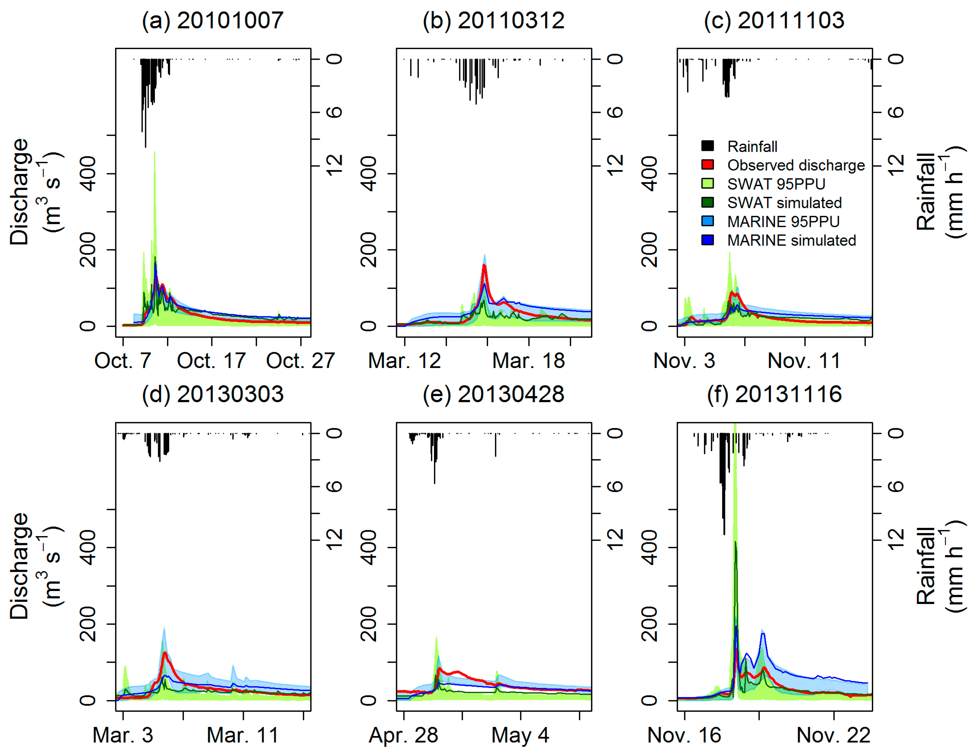
3.3.1. Discharge Simulation
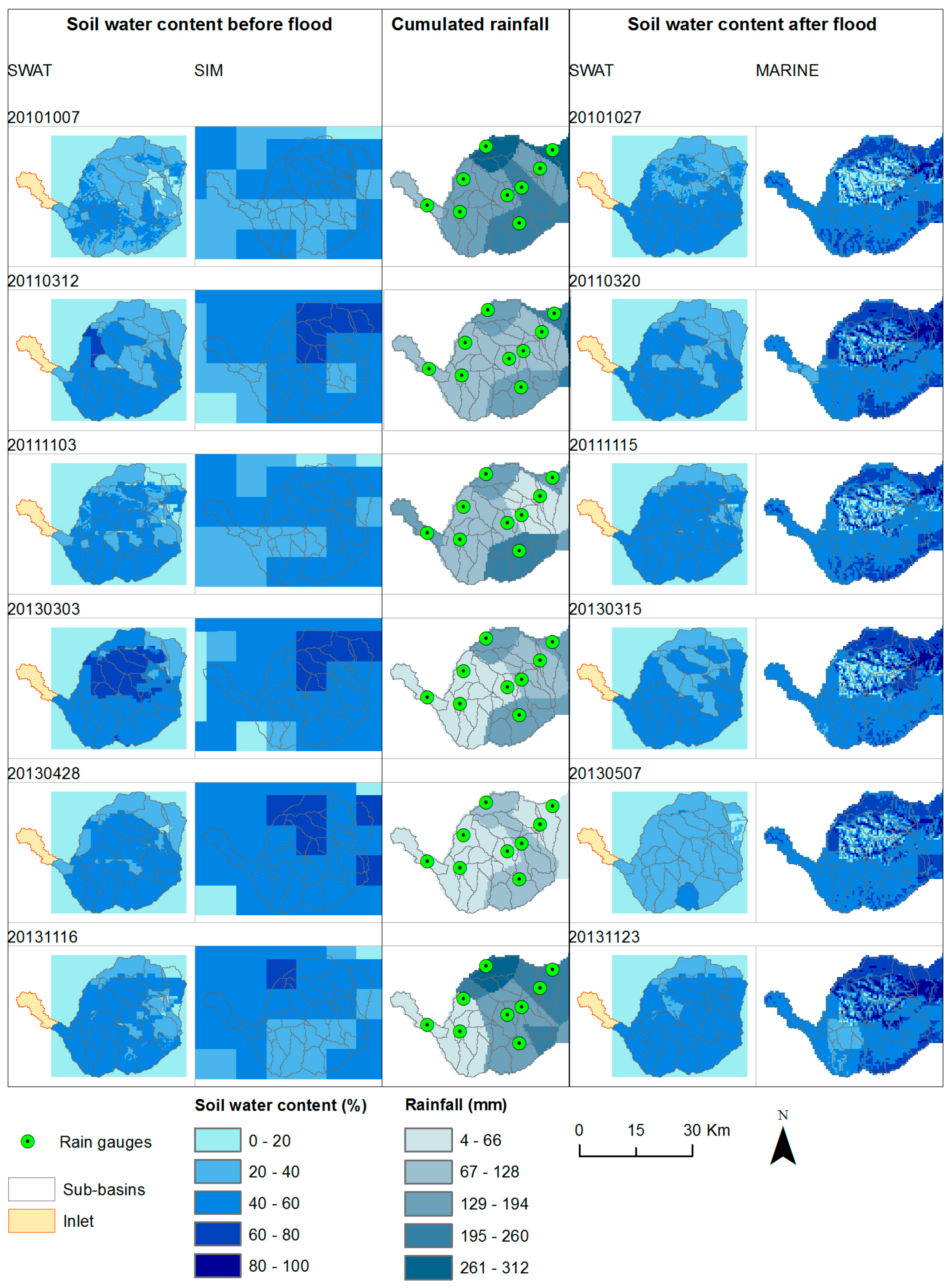
3.3.2. Soil Water Content
3.3.3. Sensitive Parameters
4. Conclusions
- During flash floods, the fully-distributed MARINE model better simulated peak discharge and peak timing, whereas the lumped SWAT model better simulated recession discharge and exported water volume;
- Overall, the latter suggests that both SWAT and MARINE performed equally satisfactorily during floods, especially considering that SWAT was calibrated and validated time-continuously over both low and high flow periods, whereas MARINE calibration and validation was focused on floods only. This also suggests that the simulation performance of the two modelling approaches was not limited by the described processes and by the different calibration procedures, but rather by the rainfall and soil data;
- Due to the limitations in rainfall and soil data, the performance of the SWAT model at the hourly time-step were not necessarily improved by the decreasing in the size of the minimum drainage area when delineating sub-basins. They were also not improved when separately calibrating a smaller sub-catchment.
Supplementary Materials
Acknowledgments
Author Contributions
Conflicts of Interest
Appendix A
- Input data: MARINE requires rainfall and soil moisture data for the initialization. SWAT requires more daily climate data to calculate potential evapotranspiration including maximum and minimum air temperature, solar radiation, relative air humidity, wind speed. In SWAT, the impact of the uncertainty related to initial soil moisture data is minimized by the use of a warm up period;
- Parameterization: SWAT is triggered by a high number of empirical parameters (23 parameters, whereas MARINE strives to offer a parsimonious model (5 parameters);
- Time discretization: SWAT is time-continuous (with a daily or sub-daily time-step) whereas MARINE is event-based (sub-daily time-step). Typically, MARINE uses a calculation time-step of 5 min (which may be adapted for numerical convergences);
- Spatial discretization: in SWAT spatial discretization is based on homogeneous units of land use/soil/slope or HRUs (lumped approach) whereas it is based on grid cells for MARINE (fully distributed approach). Hence, unlike HRUs, MARINE grid cells are connected and spatially referenced;
- Rainfall data is interpolated with Thiessen polygons in both SWAT and MARINE. SWAT associates rainfall stations to the sub-basins based on the shortest distance between each sub-basin centroid and each station. The same association is done by MARINE but with cells instead of sub-basins;
- Calibration and validation: MARINE is calibrated and validated on a number of flash flood events whereas SWAT is calibrated and validated on a continuous time period (several months to several years) including both low flow and high flow periods.
- Soil description is class-based in both models;
- The river section descriptions are different: MARINE distinguishes the main channel and the floodplain, whereas SWAT mainly considers the main channel.
- Snowfall, percolation and evapotranspiration are modelled in SWAT, not in MARINE;
- Infiltration is modelled explicitly in both models using the Green and Ampt method;
- Full hydrologic balance is computed by SWAT for each HRU and then aggregated at basin scale, whereas MARINE computes the water balance for each cell resolving the Saint-Venant and Darcy equations and then routes water from cell to cell;
- Water is routed through the channel network using the variable storage coefficient method for SWAT, the kinematic wave approximation of the Saint-Venant equations for MARINE;
- MARINE distinguishes between surface flow-generating processes (infiltration excess runoff and saturation excess runoff), not SWAT.
References
- Merz, B.; Kreibich, H.; Schwarze, R.; Thieken, A. Review article “Assessment of economic flood damage”. Nat. Hazards Earth Syst. Sci. 2010, 10, 1697–1724. [Google Scholar] [CrossRef]
- The MerMex Group. Marine ecosystems’ responses to climatic and anthropogenic forcings in the Mediterranean. Prog. Oceanogr. 2011, 91, 97–166. [Google Scholar] [CrossRef]
- The European Union (EU). Directive 2007/60/EC of the European Parliament and of the Council of 23 October 2007 on the Assessment and Management of Flood Risks; EU: Brussels, Belgium, 2007. [Google Scholar]
- Boithias, L.; Sauvage, S.; Taghavi, L.; Merlina, G.; Probst, J.L.; Sánchez-Pérez, J.M. Occurrence of metolachlor and trifluralin losses in the Save river agricultural catchment during floods. J. Hazard. Mater. 2011, 196, 210–219. [Google Scholar] [CrossRef] [PubMed]
- Boithias, L.; Choisy, M.; Souliyaseng, N.; Jourdren, M.; Quet, F.; Buisson, Y.; Thammahacksa, C.; Silvera, N.; Latsachack, K.; Sengtaheuanghoung, O.; et al. Hydrological regime and water shortage as drivers of the seasonal incidence of diarrheal diseases in a tropical montane environment. PLoS Negl. Trop. Dis. 2016, 10, e0005195. [Google Scholar] [CrossRef] [PubMed]
- Chu, Y.; Salles, C.; Cernesson, F.; Perrin, J.L.; Tournoud, M.G. Nutrient load modelling during floods in intermittent rivers: An operational approach. Environ. Model. Softw. 2008, 23, 768–781. [Google Scholar] [CrossRef]
- Reoyo-Prats, B.; Aubert, D.; Menniti, C.; Ludwig, W.; Sola, J.; Pujo-Pay, M.; Conan, P.; Verneau, O.; Palacios, C. Multicontamination phenomena occur more often than expected in Mediterranean coastal watercourses: Study case of the Têt River (France). Sci. Total Environ. 2017, 579, 10–21. [Google Scholar] [CrossRef] [PubMed]
- Roussiez, V.; Ludwig, W.; Radakovitch, O.; Probst, J.-L.; Monaco, A.; Charrière, B.; Buscail, R. Fate of metals in coastal sediments of a Mediterranean flood-dominated system: An approach based on total and labile fractions. Estuar. Coast. Shelf Sci. 2011, 92, 486–495. [Google Scholar] [CrossRef]
- Zettam, A.; Taleb, A.; Sauvage, S.; Boithias, L.; Belaidi, N.; Sánchez-Pérez, J.M. Modelling Hydrology and Sediment Transport in a Semi-Arid and Anthropized Catchment Using the SWAT Model: The Case of the Tafna River (Northwest Algeria). Water 2017, 9, 216. [Google Scholar] [CrossRef]
- Giorgi, F. Climate change hot-spots. Geophys. Res. Lett. 2006, 33, L08707. [Google Scholar] [CrossRef]
- Intergovernmental Panel on Climate Change (IPCC). Climate Change 2014: Impacts, Adaptation, and Vulnerability. Working Group II Contribution to the IPCC Fifth Assessment Report; IPCC: Geneva, Switzerland, 2014. [Google Scholar]
- Intergovernmental Panel on Climate Change (IPCC). Climate Change 2013: The Physical Science Basis. Contribution of Working Group I to the Fifth Assessment Report of the Intergovernmental Panel on Climate Change; Stocker, T.F., Qin, D., Plattner, G.-K., Tignor, M., Allen, S.K., Boschung, J., Nauels, A., Xia, Y., Bex, V., Midgley, P.M., Eds.; Cambridge University Press: Cambridge, UK; New York, NY, USA, 2013; 1535p. [Google Scholar]
- Ducrocq, V.; Braud, I.; Davolio, S.; Ferretti, R.; Flamant, C.; Jansa, A.; Kalthoff, N.; Richard, E.; Taupier-Letage, I.; Ayral, P.-A.; et al. HyMeX-SOP1: The field campaign dedicated to heavy precipitation and flash flooding in the northwestern Mediterranean. Bull. Am. Meteorol. Soc. 2014, 95, 1083–1100. [Google Scholar] [CrossRef]
- Llasat, M.C.; Marcos, R.; Llasat-Botija, M.; Gilabert, J.; Turco, M.; Quintana-Seguí, P. Flash flood evolution in North-Western Mediterranean. Atmos. Res. 2014, 149, 230–243. [Google Scholar] [CrossRef]
- Norbiato, D.; Borga, M.; Degli Esposti, S.; Gaume, E.; Anquetin, S. Flash flood warning based on rainfall thresholds and soil moisture conditions: An assessment for gauged and ungauged basins. J. Hydrol. 2008, 362, 274–290. [Google Scholar] [CrossRef]
- Garambois, P.A.; Larnier, K.; Roux, H.; Labat, D.; Dartus, D. Analysis of flash flood-triggering rainfall for a process-oriented hydrological model. Atmos. Res. 2014, 137, 14–24. [Google Scholar] [CrossRef]
- Gaume, E.; Bain, V.; Bernardara, P.; Newinger, O.; Barbuc, M.; Bateman, A.; Blaškovičová, L.; Blöschl, G.; Borga, M.; Dumitrescu, A.; et al. A compilation of data on European flash floods. J. Hydrol. 2009, 367, 70–78. [Google Scholar] [CrossRef]
- Jonkman, S.N. Global perspectives on loss of human life caused by floods. Nat. Hazards 2005, 34, 151–175. [Google Scholar] [CrossRef]
- Llasat, M.C.; Llasat-Botija, M.; Petrucci, O.; Pasqua, A.A.; Rosselló, J.; Vinet, F.; Boissier, L. Towards a database on societal impact of Mediterranean floods within the framework of the HYMEX project. Nat. Hazards Earth Syst. Sci. 2013, 13, 1337–1350. [Google Scholar] [CrossRef]
- Jeong, J.; Williams, J.R.; Merkel, W.H.; Arnold, J.G.; Wang, X.; Rossi, C.G. Improvement of the Variable Storage Coefficient Method with Water Surface Gradient as a Variable. Trans. ASABE 2014, 57, 791–801. [Google Scholar] [CrossRef]
- Jeong, J.; Kannan, N.; Arnold, J.; Glick, R.; Gosselink, L.; Srinivasan, R. Development and Integration of Sub-hourly Rainfall–Runoff Modeling Capability within a Watershed Model. Water Resour. Manag. 2010, 24, 4505–4527. [Google Scholar] [CrossRef]
- Roux, H.; Labat, D.; Garambois, P.-A.; Maubourguet, M.-M.; Chorda, J.; Dartus, D. A physically-based parsimonious hydrological model for flash floods in Mediterranean catchments. Nat. Hazards Earth Syst. Sci. 2011, 11, 2567–2582. [Google Scholar] [CrossRef]
- Jeong, J.; Kannan, N.; Arnold, J.G.; Glick, R.; Gosselink, L.; Srinivasan, R.; Harmel, R.D. Development of sub-daily erosion and sediment transport algorithms for SWAT. Trans. ASABE 2011, 54, 1685–1691. [Google Scholar] [CrossRef]
- Garambois, P.A.; Roux, H.; Larnier, K.; Labat, D.; Dartus, D. Characterization of catchment behaviour and rainfall selection for flash flood hydrological model calibration: Catchments of the eastern Pyrenees. Hydrol. Sci. J. 2015, 60, 424–447. [Google Scholar] [CrossRef]
- Garambois, P.A.; Roux, H.; Larnier, K.; Labat, D.; Dartus, D. Parameter regionalization for a process-oriented distributed model dedicated to flash floods. J. Hydrol. 2015, 525, 383–399. [Google Scholar] [CrossRef]
- Garambois, P.A.; Roux, H.; Larnier, K.; Castaings, W.; Dartus, D. Characterization of process-oriented hydrologic model behavior with temporal sensitivity analysis for flash floods in Mediterranean catchments. Hydrol. Earth Syst. Sci. 2013, 17, 2305–2322. [Google Scholar] [CrossRef]
- Arnold, J.G.; Moriasi, D.N.; Gassman, P.W.; Abbaspour, K.C.; White, M.J.; Srinivasan, R.; Santhi, C.; Harmel, R.D.; Van Griensven, A.; Van Liew, M.W.; et al. SWAT: Model use, calibration, and validation. Trans. ASABE 2012, 55, 1491–1508. [Google Scholar] [CrossRef]
- Arnold, J.G.; Srinivasan, R.; Muttiah, R.S.; Williams, J.R. Large area hydrologic modeling and assessment. I. Model development. J. Am. Water Resour. Assoc. 1998, 34, 73–89. [Google Scholar] [CrossRef]
- Furl, C.; Sharif, H.; Jeong, J. Analysis and simulation of large erosion events at central Texas unit source watersheds. J. Hydrol. 2015, 527, 494–504. [Google Scholar] [CrossRef]
- Kannan, N.; White, S.M.; Worrall, F.; Whelan, M.J. Sensitivity analysis and identification of the best evapotranspiration and runoff options for hydrological modelling in SWAT-2000. J. Hydrol. 2007, 332, 456–466. [Google Scholar] [CrossRef]
- Maharjan, G.R.; Park, Y.S.; Kim, N.W.; Shin, D.S.; Choi, J.W.; Hyun, G.W.; Jeon, J.-H.; Ok, Y.S.; Lim, K.J. Evaluation of SWAT sub-daily runoff estimation at small agricultural watershed in Korea. Front. Environ. Sci. Eng. 2013, 7, 109–119. [Google Scholar] [CrossRef]
- Bauwe, A.; Tiedemann, S.; Kahle, P.; Lennartz, B. Does the Temporal Resolution of Precipitation Input Influence the Simulated Hydrological Components Employing the SWAT Model? JAWRA J. Am. Water Resour. Assoc. 2017, 53, 997–1007. [Google Scholar] [CrossRef]
- Yang, X.; Liu, Q.; He, Y.; Luo, X.; Zhang, X. Comparison of daily and sub-daily SWAT models for daily streamflow simulation in the Upper Huai River Basin of China. Stoch. Environ. Res. Risk Assess. 2016, 30, 959–972. [Google Scholar] [CrossRef]
- Green, W.H.; Ampt, G.A. Studies on soil physics, 1. The flow of air and water through soils. J. Agric. Sci. 1911, 4, 11–24. [Google Scholar] [CrossRef]
- Mein, R.; Larson, C. Modeling infiltration during a steady rain. Water Resour. Res. 1973, 9, 384–394. [Google Scholar] [CrossRef]
- Chow, V.T.; Maidment, D.R.; Mays, L.W. Applied Hydrology; McGrawHill: New York, NY, USA, 1988. [Google Scholar]
- Sloan, P.G.; Moore, I.D. Modeling subsurface stormflow on steeply sloping forested watersheds. Water Resour. Res. 1984, 20, 1815–1822. [Google Scholar] [CrossRef]
- Arnold, J.G.; Allen, P.M. Estimating hydrologic budgets for three Illinois watersheds. J. Hydrol. 1996, 176, 57–77. [Google Scholar] [CrossRef]
- Williams, J.R. Flood routing with variable travel time or variable storage coefficients. Trans. ASAE 1969, 12, 100–103. [Google Scholar] [CrossRef]
- Overton, D.E. Muskingum flood routing of upland streamflow. J. Hydrol. 1966, 4, 185–200. [Google Scholar] [CrossRef]
- Giannoni, F.; Roth, G.; Rudari, R. A Semi-Distributed Rainfall-Runoff Model Based on a Geomorphologic Approach. Phys. Chem. Earth B 2000, 25, 665–671. [Google Scholar] [CrossRef]
- Liu, Z.; Todini, E. Towards a comprehensive physically-based rainfall-runoff model. Hydrol. Earth Syst. Sci. 2002, 6, 859–881. [Google Scholar] [CrossRef]
- Saulnier, G.M. Information Pédologique Spatialisée et Traitements Topographiques Améliorés Dans la Modélisation Hydrologique par Topmodel. Ph.D. Thesis, INP Grenoble, Grenoble, France, 1996. (In French). [Google Scholar]
- Habets, F.; Boone, A.; Champeaux, J.L.; Etchevers, P.; Franchistéguy, L.; Leblois, E.; Ledoux, E.; Le Moigne, P.; Martin, E.; Morel, S.; et al. The SAFRAN-ISBA-MODCOU hydrometeorological model applied over France. J. Geophys. Res. 2008, 113, D06113. [Google Scholar] [CrossRef]
- Tramblay, Y.; Bouvier, C.; Martin, C.; Didon-Lescot, J.-F.; Todorovik, D.; Domergue, J.-M. Assessment of initial soil moisture conditions for event-based rainfall–runoff modelling. J. Hydrol. 2010, 387, 176–187. [Google Scholar] [CrossRef]
- Vincendon, B.; Ducrocq, V.; Saulnier, G.-M.; Bouilloud, L.; Chancibault, K.; Habets, F.; Noilhan, J. Benefit of coupling the ISBA land surface model with a TOPMODEL hydrological model version dedicated to Mediterranean flash-floods. J. Hydrol. 2010, 394, 256–266. [Google Scholar] [CrossRef]
- Garcia-Esteves, J.; Ludwig, W.; Kerhervé, P.; Probst, J.-L.; Lespinas, F. Predicting the impact of land use on the major element and nutrient fluxes in coastal Mediterranean rivers: The case of the Têt River (Southern France). Appl. Geochem. 2007, 22, 230–248. [Google Scholar] [CrossRef]
- Kim, J.-H.; Ludwig, W.; Schouten, S.; Kerhervé, P.; Herfort, L.; Bonnin, J.; Sinninghe-Damsté, J.S. Impact of flood events on the transport of terrestrial organic matter to the ocean: A study of the Têt River (SW France) using the BIT index. Org. Geochem. 2007, 38, 1593–1606. [Google Scholar] [CrossRef]
- Lespinas, F.; Ludwig, W.; Heussner, S. Hydrological and climatic uncertainties associated with modeling the impact of climate change on water resources of small Mediterranean coastal rivers. J. Hydrol. 2014, 511, 403–422. [Google Scholar] [CrossRef]
- Ludwig, W.; Serrat, P.; Cesmat, L.; Garcia-Esteves, J. Evaluating the impact of the recent temperature increase on the hydrology of the Têt River (Southern France). J. Hydrol. 2004, 289, 204–221. [Google Scholar] [CrossRef]
- Jarvis, A.; Reuter, H.I.; Nelson, A.; Guevara, E. Hole-Filled Seamless SRTM Data V4, International Centre for Tropical Agriculture (CIAT). Available online: http://srtm.csi.cgiar.org (accessed on 12 November 2014).
- Rawls, W.J.; Brakensiek, D.L. A procedure to predict Green Ampt infiltration parameters. In Proceedings of the National Conference on Advances in Infiltration, Chicago, IL, USA, 12–13 December 1983; pp. 102–112. [Google Scholar]
- Durand, Y.; Brun, E.; Merindol, G.; Guyomarch, G.; Lesaffre, B.; Martin, E. A meteorological estimation of relevant parameters for snow models. Ann. Glaciol. 1993, 18, 65–71. [Google Scholar] [CrossRef]
- Quintana-Seguí, P.; Le Moigne, P.; Durand, Y.; Martin, E.; Habets, F.; Baillon, M.; Canellas, C.; Franchisteguy, L.; Morel, S. Analysis of Near-Surface Atmospheric Variables: Validation of the SAFRAN Analysis over France. J. Appl. Meteorol. Climatol. 2008, 47, 92–107. [Google Scholar] [CrossRef]
- Vidal, J.-P.; Martin, E.; Franchistéguy, L.; Baillon, M.; Soubeyroux, J.-M. A 50-year high-resolution atmospheric reanalysis over France with the Safran system. Int. J. Climatol. 2010, 30, 1627–1644. [Google Scholar] [CrossRef]
- Abbaspour, K.C.; Yang, J.; Maximov, I.; Siber, R.; Bogner, K.; Mieleitner, J.; Zobrist, J.; Srinivasan, R. Modelling hydrology and water quality in the pre-alpine/alpine Thur watershed using SWAT. J. Hydrol. 2007, 333, 413–430. [Google Scholar] [CrossRef]
- Abbaspour, K.C.; Rouholahnejad, E.; Vaghefi, S.; Srinivasan, R.; Yang, H.; Kløve, B. A continental-scale hydrology and water quality model for Europe: Calibration and uncertainty of a high-resolution large-scale SWAT model. J. Hydrol. 2015, 524, 733–752. [Google Scholar] [CrossRef]
- Abbaspour, K.C.; Johnson, C.A.; Van Genuchten, M.T. Estimating uncertain flow and transport parameters using a sequential uncertainty fitting procedure. Vadose Zone J. 2004, 3, 1340–1352. [Google Scholar] [CrossRef]
- Moriasi, D.N.; Gitau, M.W.; Pai, N.; Daggupati, P. Hydrologic and Water Quality Models: Performance Measures and Evaluation Criteria. Trans. ASABE 2015, 58, 1763–1785. [Google Scholar] [CrossRef]
- Ratto, M.; Tarantola, S.; Saltelli, A. Sensitivity analysis 1I1 model calibration: GSA-GLUE approach. Comput. Phys. Commun. 2001, 136, 212–224. [Google Scholar] [CrossRef]
- Jin, X.; Xu, C.-Y.; Zhang, Q.; Singh, V. Parameter and modeling uncertainty simulated by glue and a formal bayesian method for a conceptual hydrological model. J. Hydrol. 2010, 383, 147–155. [Google Scholar] [CrossRef]
- Li, L.; Xia, J.; Xu, C.-Y.; Singh, V. Evaluation of the subjective factors of the glue method and comparison with the formal bayesian method in uncertainty assessment of hydrological models. J. Hydrol. 2010, 390, 210–221. [Google Scholar] [CrossRef]
- Kamali, B.; Abbaspour, K.; Yang, H. Assessing the Uncertainty of Multiple Input Datasets in the Prediction of Water Resource Components. Water 2017, 9, 709. [Google Scholar] [CrossRef]
- Jajarmizadeh, M.; Sidek, L.M.; Harun, S.; Salarpour, M. Optimal Calibration and Uncertainty Analysis of SWAT for an Arid Climate. Air Soil Water Res. 2017, 10, 1–14. [Google Scholar] [CrossRef]
- Polanco, E.I.; Fleifle, A.; Ludwig, R.; Disse, M. Improving SWAT model performance in the upper Blue Nile Basin using meteorological data integration and subcatchment discretization. Hydrol. Earth Syst. Sci. 2017, 21, 4907–4926. [Google Scholar] [CrossRef]
- Rouholahnejad, E.; Abbaspour, K.C.; Srinivasan, R.; Bacu, V.; Lehmann, A. Water resources of the Black Sea Basin at high spatial and temporal resolution. Water Resour. Res. 2014, 50, 5866–5885. [Google Scholar] [CrossRef]
- Kouchi, D.H.; Esmaili, K.; Faridhosseini, A.; Sanaeinejad, S.H.; Khalili, D.; Abbaspour, K.C. Sensitivity of Calibrated Parameters and Water Resource Estimates on Different Objective Functions and Optimization Algorithms. Water 2017, 9, 384. [Google Scholar] [CrossRef]
- Gong, Y.; Shen, Z.; Liu, R.; Wang, X.; Chen, T. Effect of Watershed Subdivision on SWAT Modeling with Consideration of Parameter Uncertainty. J. Hydrol. Eng. 2010, 15, 1070–1074. [Google Scholar] [CrossRef]
- Jha, M.; Gassman, P.W.; Secchi, S.; Gu, R.; Arnold, J. Effect of watershed subdivision on swat flow, sediment, and nutrient predictions. J. Am. Water Resour. Assoc. 2004, 40, 811–825. [Google Scholar] [CrossRef]
- Hornberger, G.M.; Spear, R.C. An approach to the preliminary analysis of environmental systems. J. Environ. Manag. 1981, 12, 7–18. [Google Scholar]
- Carpenter, T.M.; Georgakakos, K.P. Intercomparison of lumped versus distributed hydrologic model ensemble simulations on operational forecast scales. J. Hydrol. 2006, 329, 174–185. [Google Scholar] [CrossRef]
- Michaud, J.; Sorooshian, S. Comparison of simple versus complex distributed runoff models on a midsized semiarid watershed. Water Resour. Res. 1994, 30, 593–605. [Google Scholar] [CrossRef]
- Moore, J.M.; Cole, S.J.; Bell, V.A.; Jones, D.A. Issues in flood forecasting: Ungauged basins, extreme floods and uncertainty. In Frontiers in Flood Research; IAHS Publication No. 305; Centre for Ecology and Hydrology, International Association of Hydrological Sciences Press: Wallingford, UK, 2006; pp. 103–122. [Google Scholar]
- Grusson, Y.; Anctil, F.; Sauvage, S.; Sánchez-Pérez, J.M. Testing the SWAT Model with Gridded Weather Data of Different Spatial Resolutions. Water 2017, 9, 54. [Google Scholar] [CrossRef]
- Omani, N.; Srinivasan, R.; Karthikeyan, R.; Smith, P. Hydrological Modeling of Highly Glacierized Basins (Andes, Alps, and Central Asia). Water 2017, 9, 111. [Google Scholar] [CrossRef]
- Braud, I.; Roux, H.; Anquetin, S.; Maubourguet, M.-M.; Manus, C.; Viallet, P.; Dartus, D. The use of distributed hydrological models for the Gard 2002 flash flood event: Analysis of associated hydrological processes. J. Hydrol. 2010, 394, 162–181. [Google Scholar] [CrossRef]
- Creutin, J.-D.; Borga, M. Radar hydrology modifies the monitoring of flash-flood hazard. Hydrol. Process. 2003, 17, 1453–1456. [Google Scholar] [CrossRef]


| Events | Dates of Flood Start and Flood End | Season | Observed | SWAT Simulated | MARINE Simulated | ||||||
|---|---|---|---|---|---|---|---|---|---|---|---|
| Peak Discharge (m3 s−1) | Time of Peak (UTC) | Volume (×106 m3) | Peak Discharge (m3 s−1) | Time of Peak (UTC) | Volume (×106 m3) | Peak Discharge (m3 s−1) | Time of Peak (UTC) | Volume (×106 m3) | |||
| 20060127 | 27/01/2006 14/02/2006 | Winter | 52 | 30/01 11:18 | 22.3 | - | - | - | 76 | 31/01 13:59 | 47.1 |
| 20101007 | 07/10/2010 27/10/2010 | Autumn | 123 | 11/10 15:59 | 38.3 | 182 | 11/10 14:00 | 54.1 | 165 | 11/10 14:35 | 62.1 |
| 20110312 | 12/03/2011 20/03/2011 | Spring | 159 | 15/03 21:16 | 21.5 | 70 | 15/03 21:00 | 15.5 | 112 | 15/03 21:16 | 31.6 |
| 20111103 | 03/11/2011 15/11/2011 | Autumn | 88 | 06/11 15:25 | 21.9 | 67 | 06/11 10:00 | 23.0 | 56 | 07/11 00:02 | 29.4 |
| 20130303 | 03/03/2013 15/03/2013 | Spring | 132 | 06/03 09:00 | 33.7 | 62 | 06/03 02:00 | 24.9 | 66 | 06/03 06:52 | 38.1 |
| 20130428 | 28/04/2013 07/05/2013 | Spring | 94 | 29/04 19:38 | 33.5 | 67 | 29/04 15:00 | 17.2 | 47 | 29/04 19:38 | 26.3 |
| 20131116 | 16/11/2013 23/11/2013 | Autumn | 165 | 18/11 01:15 | 20.4 | 416 | 18/11 01:00 | 19.3 | 196 | 18/11 01:45 | 36.0 |
| 20141128 | 28/11/2014 08/12/2014 | Autumn | 358 | 01/12 00:52 | 56.4 | - | - | - | 462 | 30/11 14:07 | 55.9 |
| Parameter | Input File | Description | Type of Change | Sensitivity Rank | Initial Ranges | Calibrated Ranges | ||
|---|---|---|---|---|---|---|---|---|
| Min | Max | Min | Max | |||||
| CN2 | .mgt | Initial Soil Conservation Service (SCS) runoff curve number for moisture condition II (-) | R | 3 * | −0.1 | 0.1 | −0.1 | 0.1 |
| ALPHA_BF | .gw | Baseflow alpha factor (1/days) | V | 16 | 0.01 | 1 | 0.01 | 1 |
| GW_DELAY | .gw | Groundwater delay time (days) | V | 12 | 0 | 500 | 0 | 500 |
| GW_REVAP | .gw | Groundwater “revap“ coefficient (-) | V | 11 | 0.02 | 0.2 | 0.02 | 0.2 |
| GWQMN | .gw | Threshold depth of water in the shallow aquifer required for return flow to occur (mm H2O) | V | 10 | 0 | 5,000 | 0 | 5,000 |
| RCHRG_DP | .gw | Deep aquifer percolation fraction (-) | V | 4 * | 0.01 | 0.99 | 0.3 | 0.99 |
| REVAPMN | .gw | Threshold depth of water in the shallow aquifer for “revap” or percolation to the deep aquifer to occur (mm H2O) | V | 18 | 0 | 750 | 0 | 750 |
| CH_K2 | .rte | Effective hydraulic conductivity in main channel alluvium (mm/h) | V | 5 * | 0 | 127 | 30 | 127 |
| CH_N2 | .rte | Manning‘s “n“ value for the main channel (m−1/3 s) | V | 1 * | 0.014 | 0.15 | 0.045 | 0.15 |
| CH_K1 | .sub | Effective hydraulic conductivity in tributary channel alluvium (mm/h) | V | 7 | 0 | 127 | 0 | 127 |
| CH_N1 | .sub | Manning‘s “n“ value for the tributary channel (m−1/3 s) | V | 14 | 0.014 | 0.15 | 0.014 | 0.15 |
| TLAPS | .sub | Precipitation lapse rate (°C/km) | V | 6 | −8 | −4 | −8 | −4 |
| PLAPS | .sub | Temperature lapse rate (mm H2O/km) | V | 2 * | 0 | 500 | 0 | 200 |
| ESCO | .hru | Soil evaporation compensation factor (-) | V | 15 | 0.7 | 0.95 | 0.7 | 0.95 |
| EPCO | .hru | Plant uptake compensation factor (-) | V | 22 | 0.7 | 1 | 0.7 | 1 |
| LAT_TTIME | .hru | Lateral flow travel time (days) | V | 13 | 0 | 180 | 0 | 60 |
| CANMX | .hru | Maximum canopy storage (mm H2O) | V | 20 | 0 | 100 | 0 | 100 |
| OV_N | .hru | Manning‘s “n“ value for overland flow (m−1/3 s) | V | 8 | 0.01 | 0.6 | 0.01 | 0.6 |
| SOL_K | .sol | Saturated hydraulic conductivity (mm/h) | R | 19 | −0.1 | 0.1 | −0.1 | 0.1 |
| SOL_AWC | .sol | Available water capacity of the soil layer (mm H2O/mm soil) | R | 17 | −0.1 | 0.1 | −0.1 | 0.1 |
| SOL_BD | .sol | Moist bulk density (g/cm3) | R | 9 | −0.1 | 0.1 | −0.1 | 0.1 |
| SOL_CBN | .sol | Organic carbon content (%) | R | 23 | −0.1 | 0.1 | −0.1 | 0.1 |
| SURLAG | .bsn | Surface runoff lag coefficient (-) | V | 21 | 0.05 | 24 | 0.05 | 24 |
| Parameter | Description | Initial Ranges | Units | Sensitivity Ranks | Fitted Values | |||||||||
|---|---|---|---|---|---|---|---|---|---|---|---|---|---|---|
| Min | Max | 20061027 | 20101007 | 20110312 | 20111103 | 20130303 | 20130428 | 20131116 | 20141128 | Average | ||||
| Correction coefficient of the soil thicknesses | 0.1 | 20 | - | 2 | 1 | 2 | 2 | 2 | 3 | 3 | 1 | 2.0 | 5.1 | |
| Correction coefficient of the hydraulic conductivities | 0.1 | 20 | - | 4 | 3 | 5 | 3 | 5 | 5 | 2 | 2 | 3.6 | 19.6 | |
| Correction coefficient of the soil lateral transmissivities | 100 | 10,000 | - | 1 | 2 | 1 | 1 | 1 | 1 | 1 | 3 | 1.4 | 1336.1 | |
| Manning’s roughness coefficient of the river bed | 1 | 30 | m−1/3 s | 3 | 4 | 3 | 4 | 4 | 2 | 4 | 4 | 3.5 | 9.2 | |
| Manning’s roughness coefficient of the flood plain | 1 | 20 | m−1/3 s | 5 | 5 | 4 | 5 | 3 | 4 | 5 | 5 | 4.5 | 15.4 | |
| Stations | Minimum Drainage Area | Time-Step | Simulation Period | p-Factor (-) | r-Factor (-) | R2 (-) | NS (-) | PBIAS (%) |
|---|---|---|---|---|---|---|---|---|
| Marquixanes | 15 km2 | Daily | Calibration | 0.86 | 1.05 | 0.65 | 0.65 | −4.7 |
| Validation | 0.85 | 0.98 | 0.66 | 0.64 | 13.5 | |||
| 15 km2 | Hourly | Calibration | 0.75 | 1 | 0.56 | 0.54 | 13.4 | |
| Validation | 0.84 | 1.05 | 0.49 | 0.45 | 7.6 | |||
| 1 km2 | Hourly | Calibration | 0.70 | 0.92 | 0.10 | −0.28 | 18.7 | |
| Validation | 0.83 | 1.05 | 0.28 | 0.21 | 0.6 | |||
| Catllar | 15 km2 | Hourly | Calibration | 0.53 | 0.79 | 0.48 | 0.46 | −34.3 |
| Validation | 0.63 | 0.83 | 0.35 | 0.32 | 17.2 |
| Model | 20061027 | 20101007 | 20110312 | 20111103 | 20130303 | 20130428 | 20131116 | 20141128 |
|---|---|---|---|---|---|---|---|---|
| MARINE | −0.55 | 0.80 * | 0.71 * | 0.60 * | 0.60 * | 0.38 | 0.39 | 0.64 |
| SWAT daily 15 km2 | - | 0.76 | 0.44 | 0.83 | 0.21 | −1.12 | 0.82 | - |
| SWAT hourly 15 km2 | - | 0.59 | 0.27 | 0.54 | 0.24 | −0.84 | −0.80 | - |
| SWAT hourly 1 km2 | - | −0.09 | −0.34 | 0.17 | −0.14 | −1.43 | −1.99 | - |
© 2017 by the authors. Licensee MDPI, Basel, Switzerland. This article is an open access article distributed under the terms and conditions of the Creative Commons Attribution (CC BY) license (http://creativecommons.org/licenses/by/4.0/).
Share and Cite
Boithias, L.; Sauvage, S.; Lenica, A.; Roux, H.; Abbaspour, K.C.; Larnier, K.; Dartus, D.; Sánchez-Pérez, J.M. Simulating Flash Floods at Hourly Time-Step Using the SWAT Model. Water 2017, 9, 929. https://doi.org/10.3390/w9120929
Boithias L, Sauvage S, Lenica A, Roux H, Abbaspour KC, Larnier K, Dartus D, Sánchez-Pérez JM. Simulating Flash Floods at Hourly Time-Step Using the SWAT Model. Water. 2017; 9(12):929. https://doi.org/10.3390/w9120929
Chicago/Turabian StyleBoithias, Laurie, Sabine Sauvage, Anneli Lenica, Hélène Roux, Karim C. Abbaspour, Kévin Larnier, Denis Dartus, and José Miguel Sánchez-Pérez. 2017. "Simulating Flash Floods at Hourly Time-Step Using the SWAT Model" Water 9, no. 12: 929. https://doi.org/10.3390/w9120929
APA StyleBoithias, L., Sauvage, S., Lenica, A., Roux, H., Abbaspour, K. C., Larnier, K., Dartus, D., & Sánchez-Pérez, J. M. (2017). Simulating Flash Floods at Hourly Time-Step Using the SWAT Model. Water, 9(12), 929. https://doi.org/10.3390/w9120929