1. Introduction
Distributed hydrologic models are useful tools for the simulation of hydrologic processes, planning and management of water resources, investigation of water quality, and prediction of the impact of climate and landuse changes worldwide [
1,
2,
3,
4,
5]. The successful application of hydrologic models, however, depends on proper calibration/validation and uncertainty analysis [
6].
Process-based distributed hydrologic models are generally characterized by a large number of parameters, which are often not measurable and must be calibrated. Calibration is performed by carefully selecting the values for model input parameters (within their respective uncertainty ranges) and by comparing model simulation (outputs) for a given set of assumed conditions with observed data for the same conditions [
7].
Hydrological model predictions are affected by four sources of error, leading to uncertainties in the results of the model. These are: 1- input errors (e.g., errors in rainfall, landuse map, pollutant source inputs); 2- model structure/model hypothesis errors (e.g., errors and simplifications in the description of physical processes); 3- errors in the observations used to calibrate/validate the model (e.g., errors in measured discharge and sediment); and 4- errors in the parameters, which arise from a lack of knowledge of the parameters at the scale of interest (e.g., hydraulic conductivity, Soil Conservation Service (SCS) curve number). These sources of error are commonly acknowledged in many studies (e.g., Montanari et al. [
8]).
Over the years, a variety of optimization algorithms have been developed for calibration and uncertainty analysis, such as the Generalized Likelihood Uncertainty Estimation method (GLUE) [
9], the Sequential Uncertainty Fitting procedure (SUFI-2) [
10], Parameter Solution (ParaSol) [
11], and Particle Swarm Optimization (PSO) [
12,
13]. Although these algorithms differ in their search strategies, their goal is to find a set of the best parameter ranges, satisfying a desired threshold assigned to an objective function. Furthermore, many objective functions have also been developed and are in common usage, such as Nash-Sutcliffe efficiency (
NSE) [
14], the root mean square error (
RMSE), the observations standard deviation ratio (
RSR) [
15], and Kling-Gupta efficiency (
KGE) [
16], to name just a few.
A comparison of the performance of hydrological models under different optimization algorithms [
17,
18,
19,
20] and objective functions [
21,
22] has been the subject of some scrutiny in the literature. Examples of this are the work of Arsenault et al. [
19], who compared ten optimization algorithms in terms of the method performance with respect to model complexity, basin type, convergence speed, and computing power for three hydrological models. Wu and Chen [
20] compared three calibration methods (SUFI-2, GLUE, and ParaSol) within the same modeling framework and showed that SUFI-2 was able to provide more reasonable and balanced predictive results than GLUE and ParaSol. Wu and Liu [
21] examined four potential objective functions and suggested SAR as a reasonable choice. In a more comprehensive study, Muleta [
22] examined the sensitivity of model performance to nine widely used objective functions in an automated calibration procedure. Less attention, however, has been paid to the optimized parameter values obtained under different optimization algorithms and objective functions, in addition to their impact on the interpretation of hydrological processes in the studied watersheds.
In this study, we examine the sensitivity of optimized model parameters to different optimization algorithms and objective functions, as well as their impacts on the calculation of water resources in two different watersheds in Iran. The current paper focuses on the GLUE, SUFI-2, and PSO algorithms and the objective functions
R2,
bR2,
NSE,
MNS,
RSR,
SSQR,
KGE, and
PBIAS (see
Table 1 for a definition of the function). To achieve our objectives, we used the Soil and Water Assessment Tool (SWAT) [
23] in the Salman Dam Basin (SDB) and Karkheh River Basin (KRB). For model calibration, we used SWAT-CUP [
24], which couples five optimization algorithms to SWAT, allowing the use of different objective functions for SUFI-2 and PSO algorithms.
3. Results
3.1. Sensitivity of Model Performance to the Objective Functions Used in SUFI-2 Algorithm
Based on the criteria of
Table 4, all objective functions performed better than satisfactory, except for
PBIAS in the calibration stage (
Table 5). In the validation, the Barak station did not have satisfactory results for six of the objective functions. This could be due to extensive water management and human activities in the upstream of Barak during the validation period.
For an illustration example, we plotted the best and the worst calibration results for the T.Karzin sub-basin in SDB in
Figure 2. The discharges based on
NSE were quite similar and close to the observation, while
PBIAS showed a systematic delay in the recession leg of the discharge.
In KRB, all objective functions performed better than satisfactory for all sub-basins except in Payepol (
Table 5). For KRB, we obtained similar results to Ashraf Vaghefi et al. [
3], who also modeled this watershed with SWAT. They reported larger uncertainties in the southern parts of the Karkheh Dam (i.e., Payepol station), because of higher water management activities. While in the northern part of the Dam (i.e., Afarine and Jologir stations), the uncertainties were smaller, and in general, model performance was better [
3].
At the Payepol station, the validation results were better than the calibration results because the Karkheh Dam was constructed after the validation period. However, the results from some objective functions like NSE and RSR were still unsatisfactory in Payepol.
To compare the closeness of the final discharges in all objective functions, we calculated the correlation coefficient table (
Table 6). The high correlation coefficients among the best simulated discharges in KRB show that most objective functions led to similar results. As in SDB, in KRB,
PBIAS displayed the worst correlation with the other methods.
We conclude here that the final results of the monthly discharges in our two case studies are not very sensitive to the objective functions in the SUFI-2 algorithm. In our two case studies, except PBIAS, other objective functions produce equally acceptable simulation results. However, this is not a general conclusion because in other regions, where, for example, snow melt is dominant, a certain objective function that targets a specific feature of the discharge may perform better and be more desirable.
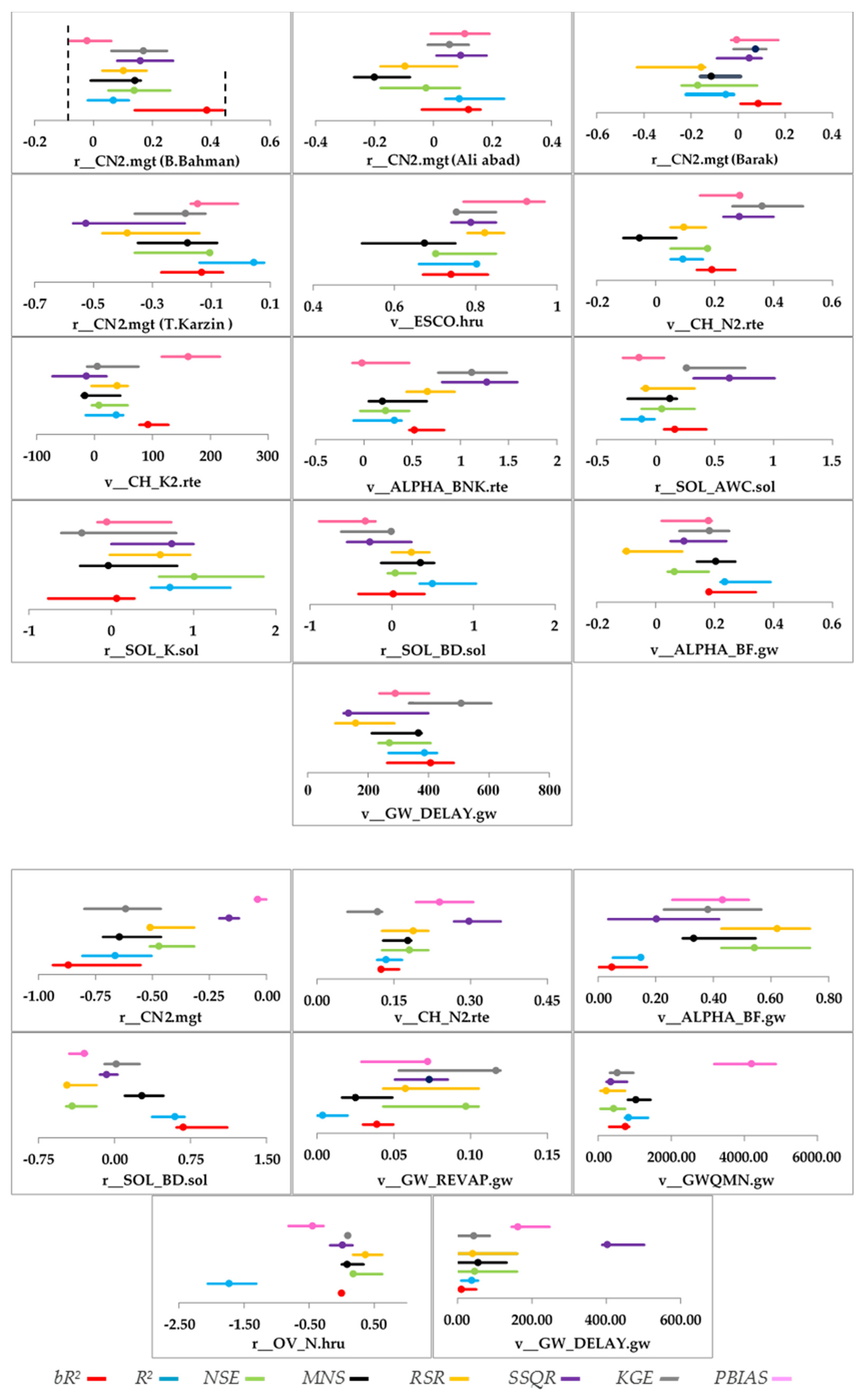
3.2. Sensitivity of Model Parameters to Objective Functions
In SUFI-2, parameters are always expressed as distributions, beginning with a wider distribution and ending up with a narrower distribution after calibration. In this study, we used a uniform distribution to express the parameter uncertainty. The parameters obtained by each objective function in the SDB and KRB study sites showed significantly different ranges (
Figure 3), even though the simulated discharges were not significantly different. This illustrates the concept of parameter “non-uniqueness” and the concept of “conditionality” of the calibrated parameters. An unconditional parameter range is a parameter range that is independent of the objective function used in calibration. By this definition, the unconditional parameter range of CN2 for B.Bahman would be the range indicated by the broken line in
Figure 3. However, this translates into a very large parameter uncertainty. This indicates that there is a significant uncertainty associated with the choice of objective functions with respect to parameter ranges.
Using the Kruskal-Wallis test, we determined which parameter ranges were significantly different from the others (
Table 7). As an example, the parameter CN2 for the upstream sub-basins of the B.Bahman outlet were not significantly different for
NSE,
SSQR, and
KGE, while they were significantly different for all other objective functions. A careful analysis of the results in
Table 7 reveals that there is no clear pattern of similarity or differences between the objective functions. However, it is clearly indicated that the
NSE method has the most common parameters with other objective functions, followed by
RSR and
KGE.
3.3. Sensitivity of Water Resources Components to the Objective Functions
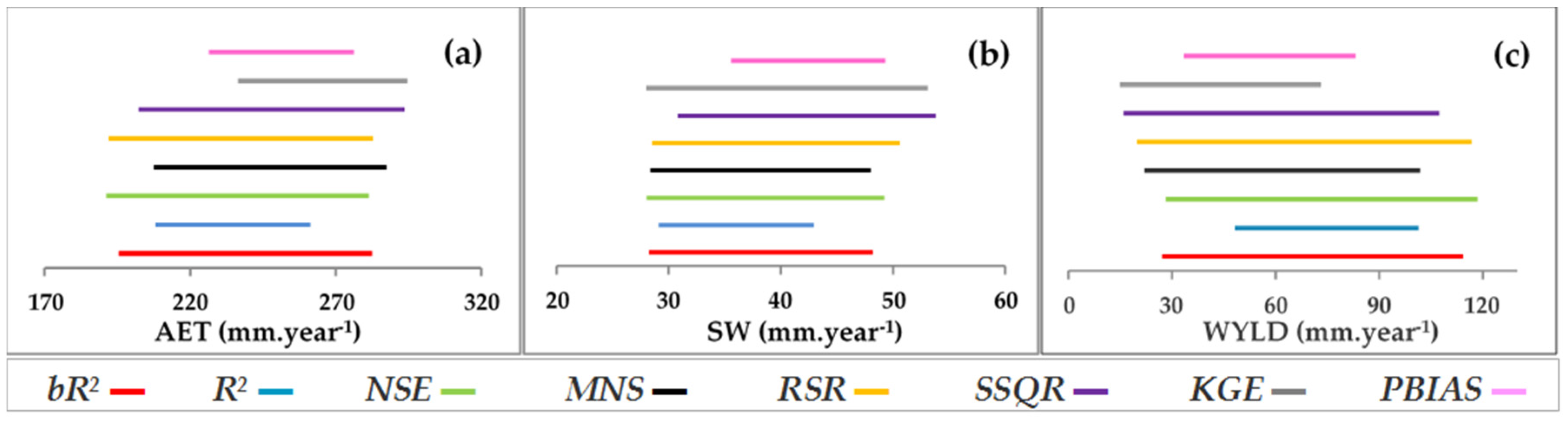
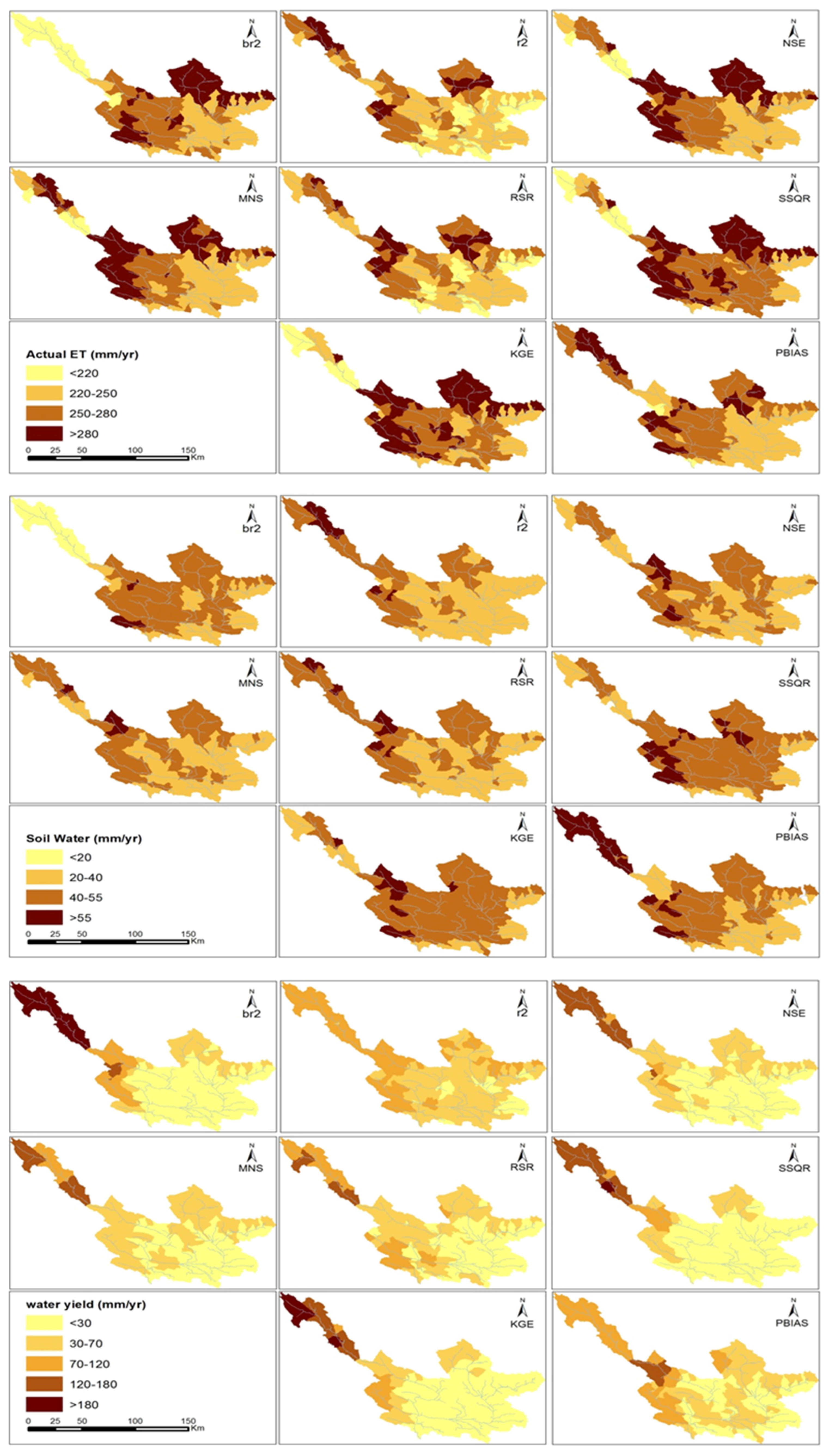
Next, we calculated the water resource components for parameters obtained by different objective functions. To show this, we calculated the actual evapotranspiration (AET), soil water (SW), and water yield (WYLD) (
Figure 4). The long-term annual averages of these variables in SDB, based on the best parameter values given by different objective functions, show significant differences. Furthermore, it is seen that the regional water resources maps of AET, SW, and WYLD exhibit significant differences in their spatial distributions (
Figure 5).
Faramarzi et al. [
2] reported a range of 120–300 mm·year
−1 in their national model for AET for the same region. In the current study, the minimum and maximum values of the annual average AET were determined by
RSR and
KGE as being 191 and 295 mm·year
−1, respectively (
Figure 4a). These values are within the uncertainty ranges reported by Faramarzi et al. [
2]. The results of SW and WYLD in SDB (
Figure 4b,c) also corresponded well with the values reported by Faramarzi et al. [
2].
3.4. Sensitivity of Calibration Performance and Model Parameters to Optimization Algorithms Using NSE
In SDB, the maximum
NSE values in all three optimization techniques were higher than 0.6; hence, they all achieved satisfactory results (
Table 8). The
p-factor values verify that most of the observed discharges were bracketed by the 95PPU of simulations by SUFI-2, followed by GLUE and PSO during the calibration and validation periods. Using a threshold value of
NSE ≥ 0.5, the SUFI-2 algorithm found 214 behavioral solutions in 480 simulations, while PSO and GLUE achieved 477 and 283 behavioral solutions in 1440 simulations, respectively. Although PSO and GLUE used a larger number of simulations, the
p-factor and
d-factor of SUFI-2 show a better performance than GLUE, followed by PSO. This would probably be expected as the latter two algorithms were not allowed to fully exploit the parameter spaces due to the limited number of runs. However, in this study, we used relatively good initial parameter values and uncertainty ranges, and all of the methods obtained quite similar and satisfactory results.
In KRB, GLUE and PSO were not successful in calibrating the SWAT model based on the defined conditions (i.e., initial parameter ranges, number of simulation runs, and behavioral threshold value), as there were no behavioral parameter sets. The SUFI-2 algorithm achieved satisfactory simulations of discharge, with
NSE = 0.53 and
NSE = 0.51 for the calibration and validation periods, respectively. The
p-factor was 55% and the
d-factor was around 1, indicating a reasonable uncertainty in the calibration and verification results (
Table 8). More than 100 behavioral solutions in 480 simulations were found with
NSE ≥ 0.5, while only three behavioral solutions were found by GLUE and no behavioral solution was found by PSO in the 2400 simulation (
Table 8). Yang et al. [
17] calibrated the Chaohe Basin in China and showed that the application of SUFI-2 based on the Nash–Sutcliffe coefficient used the smallest number of model runs to achieve similar prediction results to GLUE. Additionally, in the current study, in both watersheds, the SUFI-2 algorithm used the smallest number of runs to achieve similar results to GLUE and PSO. As already mentioned, GLUE and PSO in KRB were not allowed to fully explore the parameter spaces, which is the reason for their relatively poor performances here.
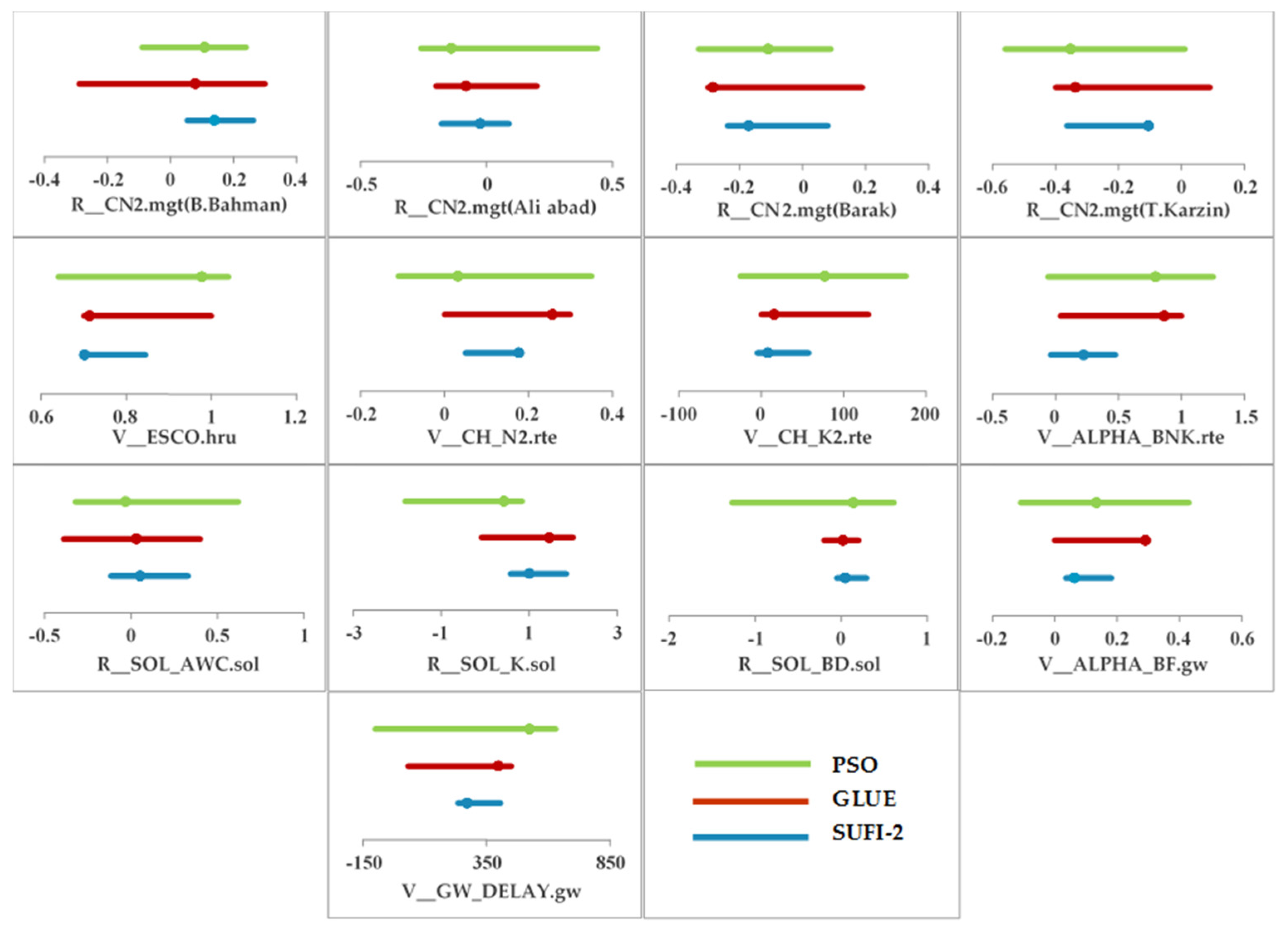
Although all three algorithms underestimated the monthly discharge at SDB, they obtained similarly good results based on the performance criteria given by Moriasi et al. [
15] (
Figure 6) and (
Table 9). The calibrated parameters estimated by the three algorithms have larger overlaps than those by different objective functions (
Figure 7). PSO provided the widest ranges of parameter uncertainty, followed by GLUE and SUFI-2.
Based on multiple comparison tests, half of the calibrated parameter ranges obtained by SUFI-2, GLUE, and PSO were significantly different in SDB. Between GLUE-PSO, SUFI2-GLUE, and SUFI2-PSO, five, four, and four parameters out of 18 were found not to be significantly different from each other, respectively. Overall, the sensitivity of the parameters to different objective functions was found to be larger than the sensitivity to optimization algorithms. This is expected because objective functions solve different problems, while calibration methods basically solve the same problem.
4. Conclusions
We investigated the sensitivity of parameters, model calibration performance, and water resource components to different objective functions (R2, bR2, NSE, MNS, RSR, SSQR, KGE, and PBIAS) and optimization algorithms (e.g., SUFI-2, GLUE, and PSO) using SWAT in two watersheds. The following conclusions could be drawn:
- 1)
In most cases, different objective functions with one optimization algorithm (in this case SUFI-2) led to satisfactory calibration/validation results for river discharges in both case studies. However, the calibrated parameters were significantly different in each case, leading to different water resource estimates.
- 2)
Different optimization algorithms with one objective function (in this case NSE) also produced satisfactory calibration/validation results for river discharges in both case studies. However, the calibrated parameters were significantly different in each case, resulting in significantly different water resources estimates.
Finally, the important message of this work is that the calibration/validation performance may not be sensitive to the choice of optimization algorithm and objective function, but the parameters obtained may be significantly different. As parameters represent processes, the choice of calibration algorithm and objective function may be critical in interpreting the model results in terms of important watershed processes.


