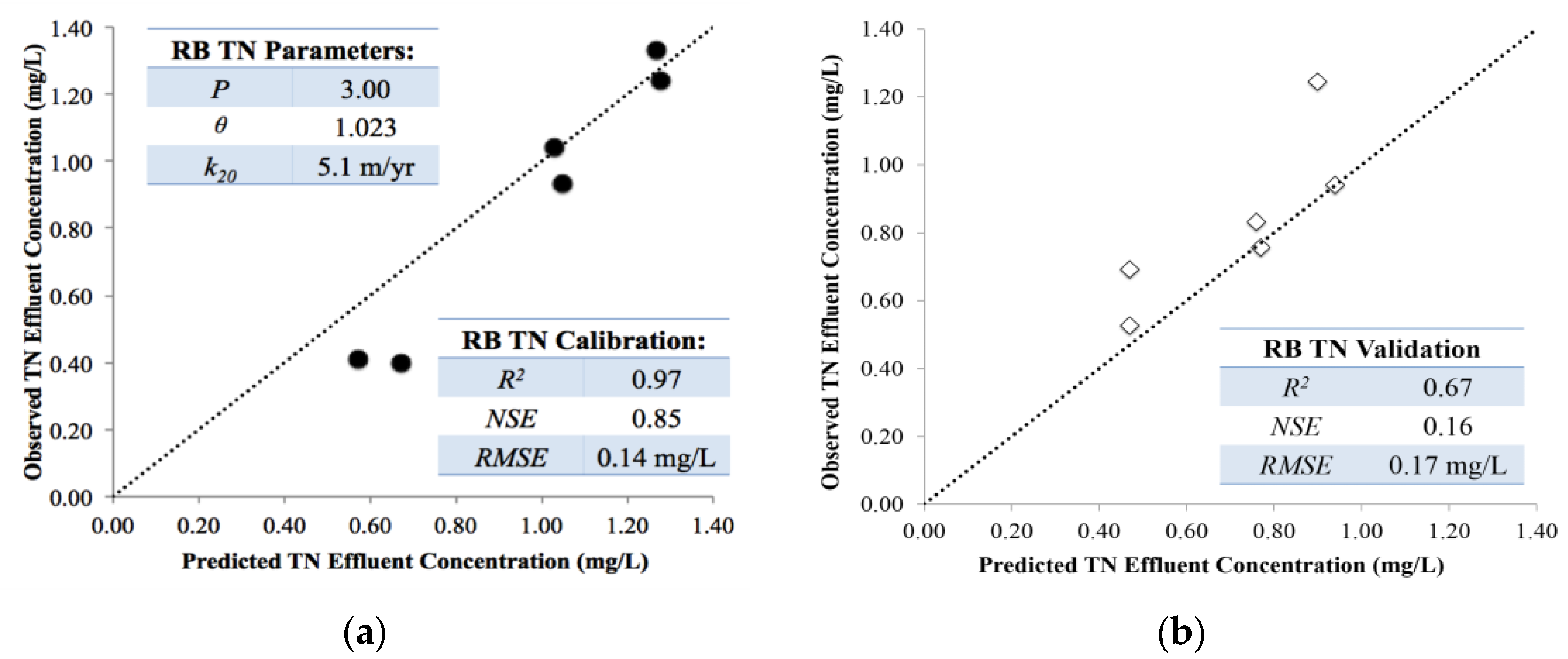
3.1. Individual CSW Calibration and Validation: Resultant Reaction Rate Parameters
Modeling fitting (reaction rate) parameters and statistical evaluations were generated for both calibration and validation datasets for each pollutant and CSW (
Figure 2). The reaction rates for each evaluation are summarized in
Table 5.
The apparent number of TIS (
P) ranged from 1.4 to 7.6 for each pollutant and CSW (
Table 6). This range fell well within the scope of tanks in series values (1–10) derived from conservative tracer experiments compiled by Kadlec and Wallace (2008) [
3] and simulations conducted by Persson et al. (1999) [
36] for treatment wetlands. The mean and median
P values ranged from 3.0 to 4.0 (
Table 5), similar to the value (3.0) recommended for initial modeling estimates and for use in treatment wetland design [
3,
36,
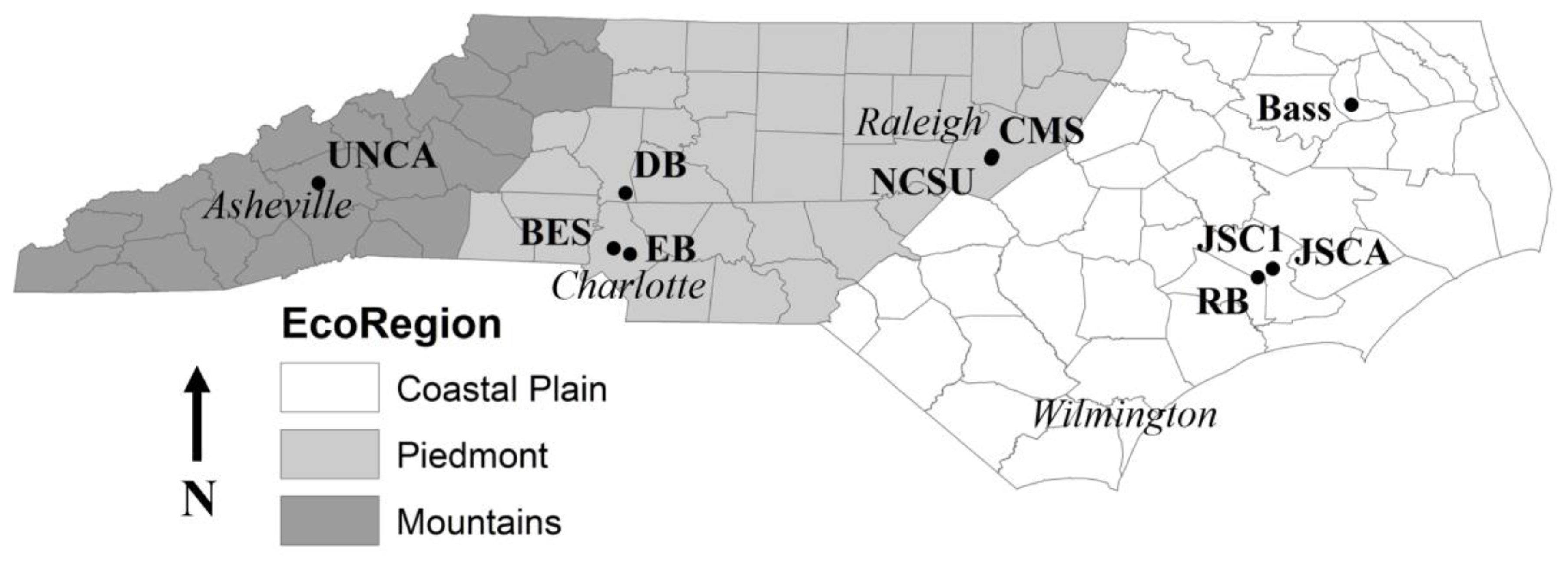
37]. Overall, the CSW sites with lower
P values (EB, DB, and JSC1), indicative of well-mixed hydrodynamics, had longer detention times relative to the other sites (
Table 4). Higher
P values suggested more short-circuiting and, typically, corresponded with deeper storage depths (CMS and Bass,
Table 4), where interactions with soil and vegetation are minimized and limit flow retardation and treatment potential [
4,
27,
36,
38].
The temperature coefficients (
θ) for pollutants derived from the field investigations varied for each CSW. The mean values for TN, TAN, TP, and TSS demonstrated temperature effects to be negligible with values of 1.007, 1.002, 1.002, and 0.993, respectively (
Table 5). In relatively warm climates, such as North Carolina, no temperature effect on TP performance has typically been observed [
3,
28,
39], and variability in TSS treatment is not usually attributed to temperature [
3]. The lack of effect of temperature on TN and TAN treatment was surprising since it has been well-documented that nitrogen processes are influenced seasonally [
21,
28,
29,
39]. However, when the TN and TAN loading to a wetland is substantially less than the growth requirements of the plants and algae (<120 and 108 g/m
2/year, [
3]), the removal of TN and TAN is mediated by the growth and decay of biomass [
29,
40]. Plant uptake rates peak in the spring and do not correspond to the annual cycle of water temperatures [
3,
29]. Therefore, in lightly loaded CSWs, water temperature and modified Arrhenius
θ values have no effect on TN and TAN removal. The mean
θ for NO
2,3-N and ON (1.024 and 1.034, respectively) reflected greater treatment at higher temperatures (
Table 6). Kadlec (2010) [
37] observed
θ values ranging from 1.035 to 1.113 for NO
2,3-N treatment in Ohio similar to that (1.043) observed in New Hanover County, NC [
3]. Stanford et al. (1973) [
41] found
θ values for ON ranged from 1.07 to 1.08, while Marion and Black (1987) [
42] observed
θ = 1.08–1.16. The NO
2,3-N and ON temperature effects herein were not as prominent as these studies. This was attributed to the smaller range of annual water temperatures observed at the USGS stream station.
The rate constants (
k20) derived from the calibration exercises resulted in a large range for each pollutant (
Table 5). The upper range primarily consisted of rate constants found for the NCSU, JSCA, UNCA sites. These sites had higher influent concentrations compared to the sites with lower
k20 values (RB and BES). Because these rate constants describe the rate a wetland can treat influent concentrations to selected background concentrations, higher values are expected for higher influent concentration. This trend does not hold when comparing rate constants for CSWs to those of treatment wetlands. The mean rate constants found in this study were higher than those found for treatment wetlands (
Table 6). For example, nitrogen values equated to the 91st (phosphorus, the 84th) percentile in the distribution of treatment wetland rate constants compiled by Kadlec and Wallace (2008) [
3]. Although treatment wetlands have higher influent concentrations compared to CSWs, treatment wetlands tend to have longer detention times and steady flow conditions compared to the flashy, episodic nature of stormwater systems [
27,
36]. Constructed stormwater wetlands yield a higher “rate of treatment” given the flashiness of their hydrology, demonstrating that rate constants are also a function of detention time and hydrodynamics (rather than solely on influent concentrations). This supports Kadlec (2010) [
37] where NO
2,3-N dynamics in pumped riverine wetlands for pulsed vs. steady flow conditions were evaluated. Rate constants observed were much higher for pulsed flow than for steady state conditions (
k20 = 107 vs. 37 m/year). The same was observed for TP in Kadlec (2001) [
43] with
k20 = 212 vs. 88 m/year for pulsed flow and steady state conditions, respectively. Few studies have been conducted to find rate constants for CSWs. Carleton et al. (2001) [
17] summarized rate constants for TP, TAN, and NO
2,3-N in 18 studied constructed wetlands receiving urban runoff. Rate constants for TP ranged from 4.9 to 46.7 m/year aligning with that observed herein (38.0 m/year), but the ranges for NO
2,3-N and TAN (3.6–57.1 and 1.0–24.6 m/year, respectively) were less than that found here (65.5 and 37.5, respectively:
Table 6). For wetlands with varying ponded surface areas and volumes, such as CSWs, Carleton et al. (2001) [
17] based their calculations on maximum values of these parameters to generate maximally conservative (that is, minimal) estimates of rate constants. This methodology could explain why their reported
k20 values were, overall, less than those derived in this study.
3.2. Calibration and Validation Results
Statistical evaluations were compiled for calibration and validation datasets for each pollutant and CSW (
Table 7 and
Table 8, respectively). Wong et al. (2006) [
20] reported the ability of a unified model (
P-k-C*) to predict stormwater treatment of various SCMs, and although no rate constants were provided, TN, TP, and TSS model fits (
RMSE = 0.08, 0.03, and 6.9 mg/L, respectively) supported this conclusion. Similar findings were observed in this study with
RMSE averages of 0.21, 0.02, and 6.85 mg/L for TN, TP, and TSS, respectively (
Table 7). The
RMSE for TN was higher than that found by Wong et al. (2006) [
20], but given the range of influent concentrations and CSW designs, the
RMSE was still relatively low. Total nitrogen and TP validation
RMSE values were similarly low: 0.20 and 0.04 mg/L, respectively; however, the
RMSE for TSS increased to 21.19 mg/L. This increase was attributed to the poor fit of one CSW, NCSU (
RMSE = 124.4 mg/L). The median was similar to results found during calibration (6.59 mg/L).
The average
R2 statistics indicated that the model explained 65–77% of the total variance in observed effluent concentrations for all pollutants (
Table 8). This range widened for the validation datasets where 24–77% of observed concentration variability was explained by the model (
Table 8). Nash-Sutcliffe model efficiency values across all pollutants ranged from 0.46 to 0.73 and −4.32 to 0.31 for calibration (
Table 7) and validation (
Table 8), respectively, where a negative
NSE signified the observed mean effluent concentration was a better predictor of effluent concentrations than the model. Both of these statistical parameters are sensitive to extreme events [
44], commonly found in the relatively small sample size of events (i.e.,
n < 8) for each individual CSW’s calibration and validation datasets.
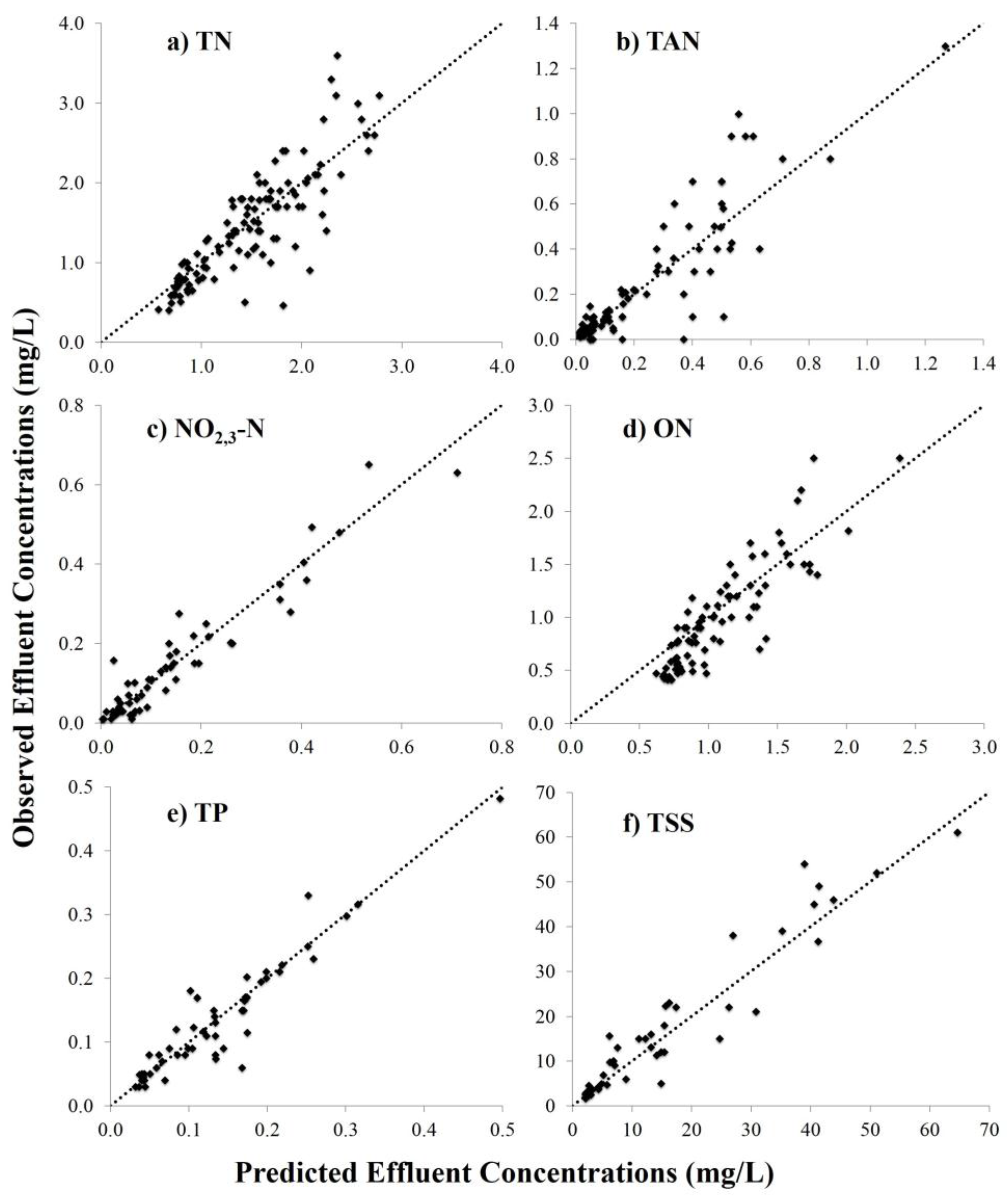
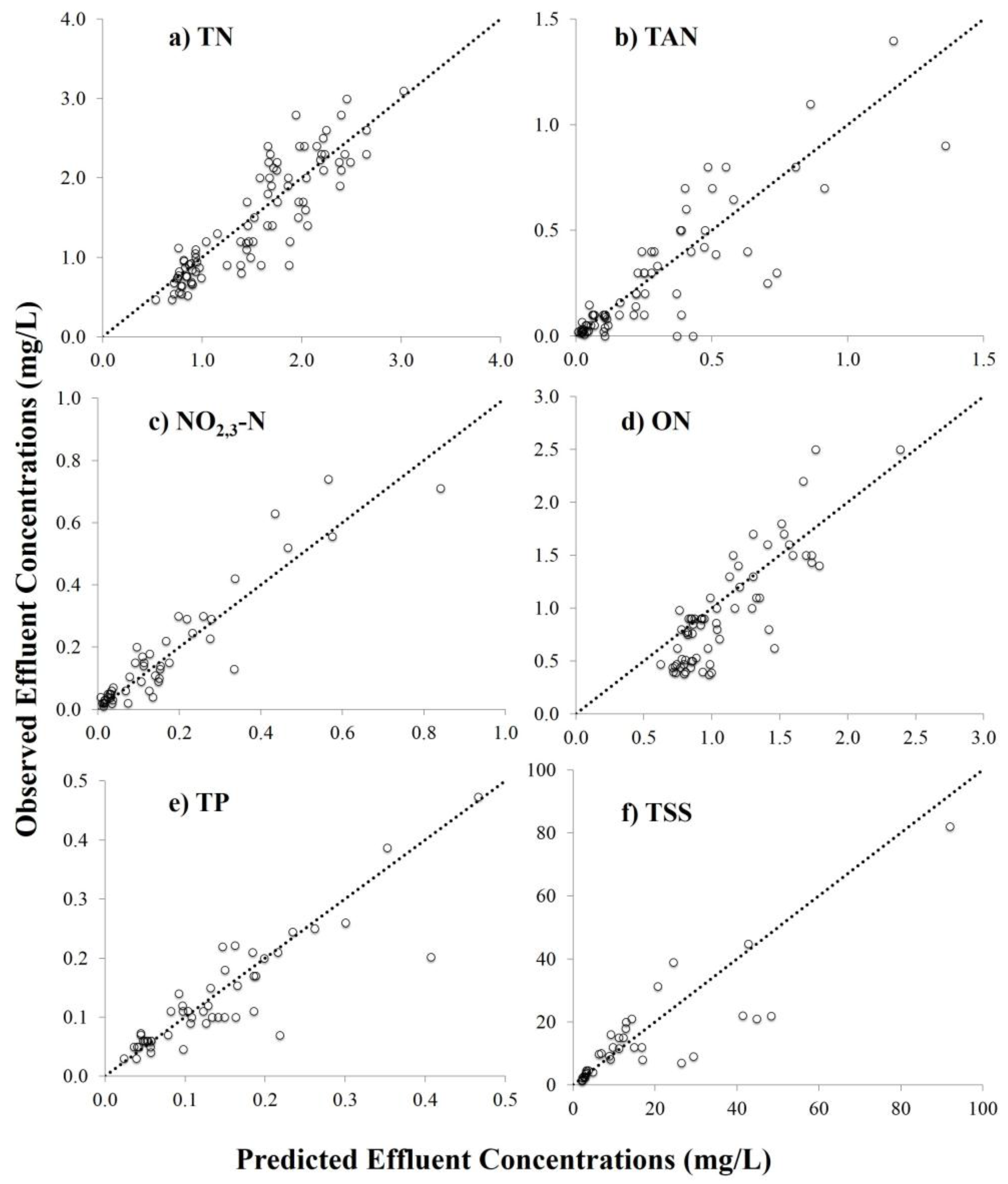
Plots demonstrating observed vs. predicted relationships for pollutant effluent concentrations from model calibration and validation events across all CSWs are compiled in
Figure 3a–f and
Figure 4a–f, respectively. Essentially, the CSWs were modeled, calibrated, and validated individually before the observed/predicted values were recompiled for an overall calculation of RMSE and NSE. The statistical metrics of all compiled CSW results for each pollutant are summarized in
Table 9.
Model prediction strength varied between calibration and validation. While events were randomly assigned to the calibration and validation data sets, those data sets were in some cases surprisingly dissimilar. For example, the TSS calibration (
Figure 3f) and validation (
Figure 4f) dataset distributions were different, even though these datasets were chosen at random. Regardless, the
P-k-C* model was typically able to describe the observed behavior well. These results: (1) suggest there is an underlying unity of a number of complex processes; and (2) support the model’s intended use for conceptual analysis and as a design tool. As an early attempt to calibrate the
P-k-C* model for use in many varying CSWs, these initial results are promising.
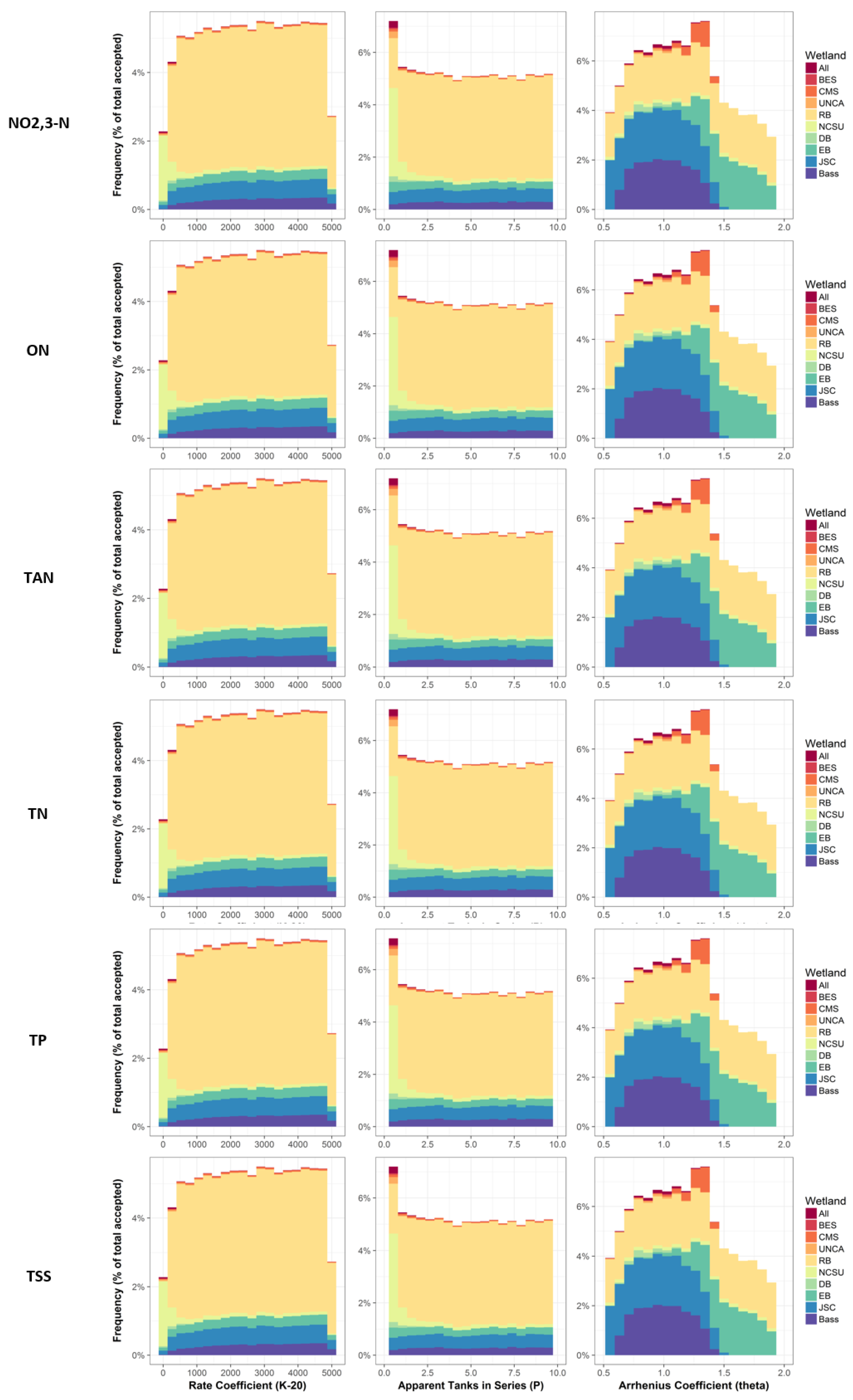
3.3. Sensitivity Analysis Results
The results of the sensitivity analysis are presented in
Figure 5. The distributions found for the Arrhenius coefficient,
θ, indicate that the model outputs were sensitive to the change in this parameter, where a
θ value of approximately 1.0 was the optimized value, although some wetlands’ optimized values were closer to approximately 1.5. The mean calibrated
θ values determined for CSWs in NC (
Table 5) fall within the optimized range determined by the sensitivity analysis (
Figure 5) and values determined by previous studies. Kadlec and Wallace (2008) [
3] cataloged
θ values of 1.002, 1.078, 1.082, and 1.043 for TP, ON, TN, and NO
2,3-N, respectively, for a wetland system studied in New Hanover County, NC. For TAN, a coefficient of 1.040 was used by Stone et al. (2002) [
28] for a livestock treatment wetland located in Duplin County, NC. Finally, total suspended solids concentration time series often display some degree of sinusoidal behavior, similar to nitrogen and phosphorus, through the course of a calendar year; however, variability in performance has not been attributed to temperature [
3]. Therefore, a temperature coefficient for TSS of 1.000 is appropriate.
The lack of a defined peak in the distribution for both
P and
k20 suggests that model outputs were not sensitive to these parameters. Kadlec and Wallace (2008) [
3] compiled tracer response curves for several surface flow treatment wetlands and found them all to be reasonably represented by
P = 3, in spite of their different geometries. Likewise, a wetland with a meandering low flow channel with full vegetation was best described as
P = 3.1 TIS in Melbourne, Australia [
36]; as was NO
2,3-N treatment in event-driven wetlands [
37]. Wong and Geiger (1997) [
14] suggested rate constants for TN and TSS of 22 and 1000 m/year, respectively, based on 59 treatment wetland systems. Carleton et al. (2001) [
17] narrowed this range in a study of removal rate constants (
k20) for 19 constructed wetland systems receiving urban runoff. Lack of sensitivity in
k20 was a surprising result. The consistent concentrations and detention times, which were relatively less than typical values for treatment wetlands, could explain why
k20 was not found to be sensitive in the model, which was a surprising result. The mean, calibrated values for
P and
k20 determined in this study (
Table 5) were similar those observed in these previous studies, supporting the wide use of these mean values due to their lack of sensitivity on model outputs. That is, these parameters can possibly be set by literature values and no longer require calibration.


