Abstract
Cadastral parcels valuation is a very important aspect when defining the priorities for the selection of newly formed parcels in the reallocation processes. Land reallocation involves a new redistribution of land parcels in the project implementation area. In doing so, it is necessary to take into account the preferences of private owners, the value of cadastral parcels, and their bonitet values, whose determination is the basic task of this research. The main goal is to propose a model to assess the bonitet of private cadastral parcels based on Expert System (ES) of fuzzy logic within the knowledge component, which would reduce uncertainty and increase the objectivity of the evaluation. Expert knowledge is included in the evaluation process by defining weighting coefficients for optimizing the rule base, and linear and nonlinear value functions for criteria standardizing. By applying the newly formed ES in the bonitet assessment, with the created base of expert knowledge, the processes of estimating attribute values have been improved, especially in the form of reducing uncertainty in the assessment of urban land parcels, as well as increasing objectivity by involving a group of experts in the model creation. The proposed model also provides equal access to all stakeholders in the process of urban renewal with different requirements and desires. The model also provides support in conducting the negotiation procedures and planning of land reallocation implementation. The proposed model was tested on the field of the construction of the Campus of University of Split.
1. Introduction
Given the diversity of spatial planning issues that occur in urban and suburban areas, urban consolidation, as a technique of planning, encompasses a wide range of procedures provided that all functional, sociological, environmental, and economic requirements are met. Therefore, its definition differs from state to state, i.e., from author to author depending on the problem to be solved while respecting its key determinants that primarily relate to the transformation of area by the development plan and protection of property and values. According to Simpson [1], urban consolidation is defined as a planning policy aimed at providing guidelines for more efficient use of existing and future resources of land and taking into account the constant growth of the population. Urban consolidation is used for area development without involving the acquisition process [2] by merging all parcels that are part of the urban consolidation area into a single land consolidation mass and redistributing land (including the possibility of compensation in cash) to all original landowners with the allocation of areas for public use as well as areas for sale to cover the costs of consolidation. Urban consolidation planning procedures require an interdisciplinary approach that includes the integration of the economy, planning, defining rights, and land management to form a comprehensive urban development strategy [3]. It can be said that urban consolidation is the key to the sustainable development of the environment, while the key to its successful implementation is found through the participation of all stakeholders in the planning and decision-making process influenced by decisions made to implement it [4]. Important to emphasize is its self-sustainable character, which benefits not only the local community, whose main task is the development of a functional urban environment, but also the inhabitants of the urban environment through its basic outcome, which is improving the quality of life. The result to strive for is the construction of a strong urban environment that successfully copes with the constant changes in society and space caused by global urbanization, the trend of which is predicted to continue in the future. A good legal framework is a basic condition for its effective implementation.
1.1. Research Focus
Analyzing the available scientific and professional literature and the legal regulations of the countries that have a long tradition of implementing urban consolidation, the advantages and disadvantages in the definition of its procedure were noticed. Based on the studied literature, new insights were gained for the definition of two key segments of urban consolidation. The first refers to the definition of the urban consolidation act that would allow owners to participate in the decision-making process, while the second refers to the definition of the urban consolidation term, which describes its characteristic procedures. The commonly used definition of urban consolidation refers to urban consolidation in the function of urban development of settlements (urban reallocation). Urban consolidation is most often carried out for areas that are developed without prior planning and where their development is not accompanied by the simultaneous development of technical and social elements of urban infrastructure. It has the priority of preserving the original position of real estate in the area of implementation (primarily related to built-up parcels). The cadastral parcels were redistributed to private owners with a percentage deduction related to the development of urban infrastructure elements (infrastructural elements of social purpose) (Figure 1).
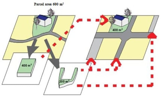
Figure 1.
Urban consolidation in the function of urban development of settlements.
Although some countries have been using these procedures for more than 100 years, unfortunately, due to the lack of planned development of cities in a large number of countries, it does not find practical application. The initial position of the built-up parcels does not provide great opportunities to improve the existing or build new infrastructure elements. The solution lies in the complete urban renewal of the whole area. Existing residential houses are being demolished, and buildings are being constructed to accommodate a larger number of residents in a smaller area (Figure 2). Unfortunately, this procedure also rarely finds practical application. The reasons are most often related to the consent of the residents for its implementation. This is also the case in Croatia where private owners have a low level of confidence in the protection of their property rights.
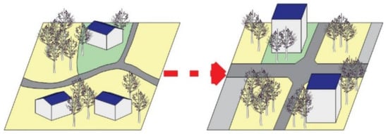
Figure 2.
Urban renewal.
The exception is urban renewal for implementation of state interest projects. With the realization of state interest projects, land reallocation is carried out from residential or residential-commercial to public land use. Most often, most of the area is used for public use, while a smaller part is left for the realization of residential buildings that allow accommodation of residents in a relatively smaller area (buildings or complexes of buildings). Given that the subject of this research is related to urban renewal, i.e., planning the implementation of a project of public interest, the consent of private owners for its launch is not necessary, but reaching an agreement for reallocation is in the interest of all stakeholders involved in its implementation. The allocation of private owners is carried out on the basis of a reallocation plan, the development of which should primarily involve spatial planners. This research will be based on defining part of the data (bonitet of cadastral parcels) needed for its development.
The reallocation process is based on data that is the product of three key elements: collected preferences of private owners, real estate valuation (includes real estate valuation before and after urban renewal), and assessing the bonitet of cadastral parcels [5]. Given that urban renewal is carried out for the purpose of implementing a large public project, land for allocation is very limited, but the formation of the land fund opened opportunities for land allocation outside the implementation area while maintaining the principle of preserving property rights and legal security. Therefore, in relation to the preferences of land owners, real estate value and parcels bonitet as well as existing land resources of investors, parcels are compared and the priority choosing of future parcels is defined.
This research is narrowed down to the development of a model to assess the bonitet of private cadastral parcels (MB). Bonitet is a generally applicable term with which it is possible to describe the quality of a business entity, the creditworthiness of a company or a client, the quality of goods in a technological and economic terms, but also land can be estimated to determine its quality, taking into account the characteristics associated with its agricultural or construction utilization [6]. Bonitet is a term that defines the difference between an “ideal” and an observed case, and is determined based on criteria identified by expert assessment. Identifying the attributes that are criteria based on which its assessment is obtained depends on the individual task as well as on the availability of data for all variant solutions (cadastral parcels). The term bonitet can be found in the Ordinance of standards for the determination of particularly valuable land for cultivation (P1) and the valuable agricultural land (P2). The basis for the valuation of P1 and P2 land, but also lower value land is based on the values of soil, climate, relief, and certain other natural conditions for agricultural production [7]. In this paper, bonitet is presented as an assessment of cadastral parcels in the process of urban renewal. The assessment of the bonitet of construction cadastral parcels determines their ratio, which defines how much better or worse an individual cadastral parcel is compared to other land plots. The main goal is to propose a model to assess the bonitet based on an expert system of fuzzy logic which would reduce uncertainty and increase the objectivity of the evaluation. The main hypothesis is whether it is possible to improve the planning of urban renewal by appropriate design of the model to assess the bonitet of cadastral parcels based on fuzzy expert system. The research is related to the project planning of the construction of the Campus of the University of Split.
After reviewing the literature and defining the research focus, the second chapter (Materials and methods) gives the general form of the model as such is adaptable to another research area (by adding or removing criteria for bonitet assessment). The model was validated in the Campus area, and the results are presented in Chapter 3. Answers to the set hypothesis and goals are given in the Conclusion together with the recommendations for further research.
1.2. Literature Review
Urban consolidation involves a new reallocation of parcels in the project implementation area. As said above, it is necessary to take into account the preferences of private owners, the real estate values, and their bonitet values, whose determination is the basic task of this research. Given that the proposed approach requires the inclusion of a large amount of data as well as different stakeholders with their own preferences, there is a need to implement a system that will support decision-making. In the existing scientific and professional, as well as legislative literature, no approach has been found to evaluate the bonitet of cadastral parcels for the purpose of fairer urban reallocation. Most often, the urban reallocation process is the result of a spatial planner’s study taking into account the preferences of private owners. Unfortunately, a more detailed insight into the whole procedure was not found in the existing literature. The conclusion is that the whole procedure is still based on subjective assessment. The initial questions:
- Is it possible to develop a model that will provide an approach to the valuation of existing urban land parcels, with a view to a fairer reallocation process?
- Is it possible to develop a flexible model that will be able to adapt to another research area?
- Is it possible to increase objectivity when adopting a reallocation plan?
The research of the existing literature moved in the direction of seeking solutions to the questions asked. The initial goal of this research was to study methods and systems to support decision-making in solving any other kind of spatial issue, whether it is agricultural or urban land. The state of the existing scientific literature related to land valuation is given below, which served as the basis for the development of the MB.
Kilić et al. [8] developed a model of index fragmentation assessment. They proposed a methodology to assess the urban land fragmentation during the implementation of sustainable Urban Renewal. Particular importance is attached to the issue of ownership within the area of construction, which, along with the financial segment, is the main limiting factor for the realization of the project. The spatial distribution of private parcels, their relationship, and utility to the larger whole they belong to are the basis for defining the influential criteria to assess the index fragmentation. The methods used to solve the task are Simple Additive Weighting method (SAW) for ranking alternative solutions, i.e., cadastral parcels, spatial elements, and areas of future construction, and Fuzzy Analytic Hierarchy Process method (FAHP) for defining the criteria weights. This model is part of a large study divided into four phases, and itself belongs to the 3rd phase of the urban consolidation implementation. The research presented in this paper is part of the 4th phase of the implementation, which refers to land reallocation processes.
Branković et al. [9] propose a methodology for land assessment in the GIS environment and the application of GIS techniques and technology as a primary tool in the evaluation of agricultural land in the land consolidation process. Demetriou et al. [10] state the reasons for the development of a new decision support system (DSS) for designers when planning the land consolidation process and finally provide a prototype framework for the proposed system. Uyan et al. [11] state that the core of the land consolidation problem is land reallocation. They developed a model of agricultural land reallocation based on the spatial DSS (SDSS), compared its results with conventional methods, and tested it with agricultural production stakeholders. Cay and Uyan [12] proposed the expression of stakeholder preferences with weight coefficients determined by the AHP method in the process of reallocation in land consolidation. Zou et al. [13] used SDSS with integrated fuzzy logic in assessing the potential of land consolidation through four key factors: the efficiency potential of new aggregated arable land, the potential to improve productivity, the potential to reduce production costs, and the potential to improve the environment. Kilić et al. [6] developed an expert fuzzy logic system that improved and optimized the process of the relative valuation of agricultural land as one of the critical steps in the implementation of land consolidation. The proposed expert system provided effective support in conducting the negotiation procedures and planning of land consolidation implementation with the involvement of different stakeholder groups with different requirements and wishes. Cay et al. [14], Cay and Iscan [15], Cay and Iscan [16], Cay and Iscan [17], and Kagita et al. [18] dealt with the application of fuzzy logic in land reallocation procedures. Ertunca and Cay [19] used it in an inland classification processes.
For the definition of the MB, which is the subject of this research, fuzzy logic was applied to make decisions in intelligent and transparent way. The integration of the fuzzy logic into the decision-making processes was found only in the assessment in agricultural land consolidation procedures, while its application in the classification of land in urban consolidation was not found. Certainly, the biggest reason contributing to the still insufficiently researched possibilities of optimizing and objectifying urban consolidation procedures lies in the complexity of the procedure itself and the need to consider a much larger number of influential parameters. Fuzzy logic enables the implementation of expert, engineering experience of a particular process into the inference algorithm. The objectivity of inference is achieved by including a larger number of experts in the process of defining an expert system, which is why those, most often, small differences in expert thinking define fuzzy data sets. The proposed model was tested on the field of the construction of the Campus of University of Split.
2. Materials and Methods
Assessing the bonitet values of cadastral parcels is an important segment when defining the priorities for the selection of newly formed real estate in the reallocation processes. In doing so, a list of bonitet values of cadastral parcels will be defined as a result of this research. Figure 3 shows the implementation of fuzzy logic for defining a MB in Urban Renewal processes. The diagram is divided into two parts; the first part refers to preparatory procedures and implementation procedures.
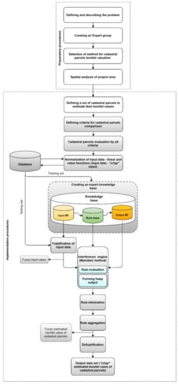
Figure 3.
Model to assess the private cadastral parcels bonitet.
2.1. Preparatory Procedures
Preparatory procedures include steps defining and describing research problems, forming an expert group, selection a method for cadastral parcels bonitet valuation, and spatial analysis of the research area. The main goal is to define a model to assess the bonitet of private cadastral parcels. Given that the initial requirement was to increase objectivity in decision-making, a group of experts was engaged who participated in the creation of all the steps of this model. Experts were selected according to their scientific and professional experience in solving similar spatial problems. The next step is the choice of method which is determined by expert judgment. Experts agreed to choose the method that should have enabled the modeling of expert knowledge in a form understandable to the computer language that would objectify the decision-making process, and the procedure itself could be applied in solving similar spatial tasks. Based on the defined requirements, the fuzzy logic method is selected, as part of artificial intelligence that enables modeling of human knowledge into mathematical form. The goal of artificial intelligence methods is to turn the human way of thinking into an algorithm by applying appropriate mathematical methods [20].
ESs have evolved primarily from the need to provide problem-solving and decision-making assistance to non-expert users in a particular field who require expert support. This particular system is usually limited to narrow applications, and its use for tasks that exceed the domain of its definition can result in inaccurate and poor quality data unsuitable for later use. The selected ES is the fuzzy logic method. Fuzzy logic is based on the embedding of human knowledge through the form of a set of rules into algorithms which allow mathematical analysis of a given problem. The difference between classical set theory and fuzzy set theory is in the way an element belongs to a particular set [21]. While in classical theory, the element either belongs or does not belong to a set, in fuzzy set theory the degree of belonging of an element to a particular set is defined, which is called fuzzy set. In the following, the mathematical basis of fuzzy logic will be presented through steps adapted to the problem of this research. Although the problem of fuzzy logic dates back to history, its creator is considered to be Lotfi Zadeh who introduced the idea of fuzzy or “soft” belonging to sets when describing individual phenomena or features [22]. Zadeh explored the possibility of transforming human knowledge, often expressed in words that cannot be clearly and precisely defined, into a computer-understandable form. As human language is difficult to translate into absolute terms, 0 or 1, there is a need to develop logical models that will know how to handle such knowledge [23]. The final step is spatial analysis of project area. The attributes of cadastral parcels were identified, based on which the criteria for their comparison will be defined. The definition of criteria, the manner of assessing cadastral parcels according to them, the relationship according to their importance, and bonitet assessment are obtained based on the assessment of experts involved in the decision-making process.
2.2. Implementation Procedures
The first step of the implementation procedures concerns the definition of cadastral parcels set to assess their bonitet values. The following steps, which are grey colored, define fuzzy logic algorithm.
The fuzzy logic algorithm is defined in ten key steps:
- Defining criteria for cadastral parcels comparison (input data), linguistic variables and terms (initial phase)
- Cadastral parcels evaluation by all criteria
- Normalization of input data—linear and value functions (input data—”crisp” input)
- Defining membership functions—MFs (initial phase)
- Defining the rule base in the knowledge base (initial phase)
- Conversion of input crisp values into fuzzy values using MFs (fuzzification)
- Evaluation of rules (inference mechanism)
- Combination of results according to each rule (aggregation)
- Conversion of output fuzzy values into their crisp values (defuzzification)
- Output data set (“crisp” estimated bonitet value of cadastral parcels)
Each of these steps will be explained in more detail below.
Step 1—Defining criteria for cadastral parcels comparison (input data), linguistic variables, and terms (initial phase)
With the definition of cadastral parcels set and their initial analysis, the criteria for their comparison need to be identified. The choice of criteria depends on the specific task, and their general set includes the following criteria: construction utility, orientation, access to the registered road, distance from main roads, micro-locations, infrastructure, aspect, slope, shape, ecology, vegetation, and compliance between cadastre and land registry. As the proposed methodology is flexible, depending on the specific task, the criteria can be added or removed from the initial set of criteria.
There are two types of input data in fuzzy logic processes: The first type refers to phenomena that are qualitatively described and define fuzzy ranges that have unclear numerical boundaries, while the second type refers to phenomena that can be expressed numerically (parcel shape, distance from main roads), but their classification is based on an expert judgment that cannot be determined by a simple mathematical model. In the second case, which is the case in this research, fuzzy sets are defined based on their numerical values. They are joined to linguistic variables for simplicity of presentation. They represent fuzzy sets that are determined by membership functions depending on the character of individual data that are grouped (countable or innumerable, discrete, or continuous), or the type of domain over which they are assigned.
Step 2—Cadastral parcels evaluation by all criteria
In this step, the evaluation of cadastral parcels is performed according to the defined criteria. The data set is divided into training and testing sets. One of the advantages of fuzzy logic is the possibility of its application in cases where there are uncertainty and inaccuracy of any kind. Given the above, fuzzy logic can be used in cases when it is difficult to determine the measure of the data, i.e., when there is not enough recorded input data required for quantitative analysis.
Step 3—Normalization of input data—linear and value functions (input data—“crisp” input)
For combining and comparing the defined criteria with each other, it is necessary to normalize the input data, i.e., to reduce their values to relation from 0 to 1. Sometimes the relationship between source data and their normalized values is much more complex and cannot be described by a linear function. For this reason, the normalization (or standardization) of certain criteria is carried out by applying value functions that are not only related to information, but also the experiential judgments of experts involved in its definition. Creating value functions is an important and complex task because their values directly affect the accuracy of later calculations [24]. Value functions are the result of a specially designed interview conducted between decision-makers and experts involved in the decision-making process [24]. In this research, the direct value rating method was chosen for defining value function.
Direct value rating involves the following five steps for each criterion [24,25]:
- Selection of the score range for a criterion, i.e., the ideal or goal value (i.e., maximum value) and the minimum value which corresponds to values of 1 (best) and 0 (worst), respectively.
- Definition of the qualitative characteristics of the value function, i.e., monotonicity, convexity, concavity, etc.
- Assignment of values for selected criterion scores that have been defined by dividing the attribute range into 3 to 6 equal intervals resulting in 4 to 7 points, respectively.
- Fit a mathematical equation through these points using appropriate software (interpolation, curve adjustment).
- Consistency checks to confirm the validity of the functions as representations of preference.
Step 4—Defining MFs
Defining MFs also belongs to the initial phase of the fuzzy logic algorithm, and together with the rule base, it forms an expert knowledge base. For each input variable, it is necessary to determine a certain number of fuzzy sets and their MFs. A triangular MF was selected. The number of membership functions of the input and output variables, as well as their shape, is the result of an agreement between the experts involved in the decision-making process. As the shape of the membership functions does not have a large influence on the functioning of the model, attention should be paid to the choice of the number of membership functions of the input and output variables. The decision is made by selecting the minimum number of membership functions that describe the variables precisely enough (the speed of the system should be optimal). Membership function together with a rule base form knowledge base.
Step 5—Defining the rule base in the knowledge base
By forming specific rules that define the relationship between the input and output values the case of insufficient input data is covered; the output values are much more precise than with the application of mathematical models whose analysis results directly depend on the density of the available input set. The set of language rules that determine the output value is called the rule base. Expert knowledge is modeled by fuzzy rules. It can be said that the rule base stores the empirical knowledge of experts who, according to their expertise in a particular field, are involved in the decision-making process. Knowledge base includes rule base and membership functions of the input and output variables. This step involves two actions:
(a) Optimizing the development of the rule base
The first action refers to the proposal of the methodology to optimize the process of creating a complex rule base for the bonitet assessment in the implementation of Urban Renewal. Creating a rule base is a complex and time-consuming process. Given the above, efforts need to be focused on defining the optimal number of rules for describing a particular problem. The total number of rules, i.e., the total number of combinations of fuzzy sets of input variables, is obtained according to the expression
where Z represents the total number of rules, while represents the total number of MFs, i.e., fuzzy sets for each input variable . Although the optimal number of input variables is from 3 to 5, it is often necessary to define a larger number of inputs due to the specificity of each task and several elements influencing its definition, which, in proportion to the number of MFs, increases the number of rules that need to be determined. When defining the number of MFs of each input variable, it is necessary to start from their minimum value, i.e., from number three. However, although the reduced number of MFs affects the reduction of the number of rules, and thus the system speed, their smaller number must not result in an incomplete description of input variables.
All this affects the complexity of the fuzzy system, and determining the number of rules whose number can exceed tens of thousands, as well as maintaining consistency in defining them becomes a very difficult, almost impossible task. Although the scientific literature states that the definition and the optimal number of fuzzy rules is an expert judgment [26], during this research, the absence of a methodology that would enable the definition of systematic and logical relationship of input and output variables, and thus facilitate and accelerate expert assessment can create a major obstacle when performing a task. The fact that each of the input variables does not have an equal influence on the definition of the output variable should also be taken into account. Thus, already during the initial set-up of the system, which included the definition of criteria, it was noticed that their ratio is not equal and that accordingly they cannot be observed in the same way, i.e., with a definition of equal importance.
These reasons influenced the need to define the methodology proposed by this research, which is based on expert assessment of weighting coefficients that will take into account the definition of the relative ratio of input variables, and on the other hand, allow logical connection of input and output values. The aim of the methodology is to optimize the rule base.
The weights of the input variables were defined using the AHP method. Each expert involved in the research separately conducted the assignment of weights that were entered into the weight matrix:
where (i = 1, 2, …, n) represents the input variable, and (k = 1, 2, …, m) represents the expert involved in the research. Each row of the matrix represents the estimated weight assigned by one expert to each input variable, while each column represents one input variable with the assigned weights. The final weight for each input variable is obtained by summing the values of the weights by columns using the expression for the ordinary arithmetic mean:
where is the final weight of each input variable , is the sum of the weights assigned by the experts for each input variable , and m is the number of experts involved in the assessment.
Weights are normalized by percentage normalization and the final weighting factor for each input variable is
where is the normalized weight of the input variable , is the weight of the input variable , and is the total sum of the weights of all input variables. The sum of all normalized weights should be equal to one.
Each input variable (i = 1, 2, …, n) is associated with a number of fuzzy sets represented by the MFs of the input variables , and each output variable (i = 1, 2, …, d) is associated with a number of fuzzy sets represented by the MFs of the input variables . The output value of a variable is a function of the input values of the variable , i.e., the output function of the membership of an individual variable is a function of the input functions of the membership of the variable . To define which fuzzy set of output variables belongs to a particular combination of fuzzy sets of input variables, the expression is used:
where represents the standardized ordinal number of the fuzzy set of each input variable, and represents the weighting coefficient for defining the ordinal number of the fuzzy set of the output variable. The coefficient range is from 0 (for cadastral parcels whose standardized input values of each variable are in the first, worst fuzzy set) to 1 (for cadastral parcels whose standardized input values of each variable are in the last, best fuzzy set). Depending on the number and shape of the class of the output variable, the distribution of the coefficient according to its fuzzy sets is defined.
By applying the methodology of optimizing the definition of the connections of input and output variables, several advantages were observed, primarily related to shortening the time of defining the rule base, as well as maintaining consistency in the expert assessment of defining rules of many different fuzzy sets variables combinations. As the rule base together with the MFs defines the knowledge base of the fuzzy logic system, the expert knowledge in the proposed methodology primarily referred to defining the relative relationship of input variables, respectively their weighting coefficients to optimize the definition of a combination of input and output fuzzy sets. Likewise, and especially in complex systems characterized by a large number of input variables and their fuzzy sets, the proposed methodology eliminates inconsistencies in defining a large number of rules, thus increasing certainty in the correctness of their inference.
(b) Defining basic operations on fuzzy sets
Finally, it is necessary to define the basic operations on fuzzy sets, i.e., the ways of defining the connections of the conditional part of the rule with its conclusion. Given the specificity of the task, it was decided to use the T-norm as the basic operation on the sets.
Step 6—Conversion of input data crisp values into fuzzy values using MFs (fuzzification)
The process of converting crisp values of input data into their fuzzy values is called the fuzzification or softening process. Fuzzification is the process of modeling the numerical values of input variables into the appropriate form of the degree of belonging to one or more fuzzy sets appropriate to the fuzzy decision-making process [27].
Step 7—Evaluation of rules (inference mechanism)
The process of transformation of input fuzzy sets into output fuzzy sets is called the process of inference, and is carried out in two steps:
- Selection of inference operators.
- Application of the implication method, which is divided into:
- (a)
- Determining the resulting degree of membership of the conditional part of the equation,
- (b)
- Determining the output set.
Fuzzy systems can be divided into two categories depending on the inference mechanism [28]:
- -
- Global system: the whole database of rules is used, and the accuracy of the relation depends on the discretization density of the domains of input and output variables.
- -
- Local system: only those rules that are relevant to the value of the input variables are used.
In the research presented in this paper, the Mamdani model of local fuzzy inference was used. Its process involves steps 7, 8, and 10 of the fuzzy logic algorithm.
Depending on the fuzzy values of the crisp input data (Step 6) and the choice of the local inference model, the generated rule base was optimized, i.e., the elimination of redundant rules that burden and slow down the system was performed. The rules were eliminated in two cases:
- -
- As all possible combinations of fuzzy sets of input data are determined when defining the rule base, those rules that do not correspond to the defined data set for which the research is conducted are eliminated from the rule base and thus do not affect the output values.
- -
- Redundant rules are eliminated, i.e., those rules that refer to the same combination of fuzzy sets of input variables.
Step 8—Combination of results according to each rule (aggregation)
The aggregation of all fuzzy output sets, to which the truncation and scaling techniques were previously applied, into a single fuzzy set of each output variable was performed using an aggregation operator. For this research, the Mamdani inference operator was chosen. Mamdani inference operator or max-min operator is a combination of minimum T-norm for implication and maximum T-conorm for aggregation and is defined by the expression [29]
By applying the Mamdani inference operator, the resulting fuzzy set is formed as a union of previously defined segments and the reduction of the output sets of all valid rules.
Step 9—Conversion of output fuzzy data values into their crisp values (defuzzification)
Defuzzification is the process of obtaining a resultant crisp number from the output of the aggregated fuzzy set. Different methods of fuzzy–crisp conversion are used to determine the crisp output value, and for this research the Center of Gravity method was chosen. The Center of Gravity method, i.e., centroid method represents the center of gravity of a geometric figure defined by the resulting fuzzy set of an individual output variable. The crisp value of the output variable is obtained through the expression [30].
where is the degree of membership of the aggregate output variable z with a fuzzy set C. The Centroid method due to good interpolation properties is the most commonly used defuzzification method.
The highest value of membership to the n-set is obtained as [30].
Implementation procedures were completed with a process of defuzzification, and the result are cadastral parcel bonitet values.
Step 10—Output data set (“crisp” estimated bonitet value of cadastral parcels)
Given that cadastral parcels are assessed in relation to the reference values of the criteria, the result is an assessment of the bonitet from 0 to 1, where the total grade of 0 is given to the cadastral parcel that received a grade of 0 according to all defined criteria. Opposite of that, the total grade of 1 is given to the cadastral parcel that received a grade of 1 according to all criteria.
The AHP Method
The AHP method is one of the most applied multicriteria decision-making methods. It is used to determine the ranking of alternative solutions that have been evaluated according to predefined criteria. In addition, it allows the determination of importance factors (weight) for several stakeholders or groups of stakeholders involved in the decision-making process. Stakeholders are most often formed into groups according to the common preferences they share. The weights of criteria are of a subjective nature, and the way of determining the final weight for each group of stakeholders is a matter of mutual agreement of the stakeholders. The final score for each alternative solution is obtained by combining the weights and the evaluation of alternative solutions.
At the very beginning, it is necessary to create a pairwise comparison matrix A which has dimension n × n (n is the number of considered evaluation criteria). Its purpose is to calculate the weights of different criteria. Element ajk defines relationship j-th to k-th [31]:
- -
- ajk > 1—j-th criterion is more important than the k-th criterion,
- -
- ajk < 1—j-th criterion is less important than the k-th criterion,
- -
- ajk = 1—j-th and k-th are equal important.
The Saaty [31] numerical evaluation scale is used to measure the relative importance between criteria. After defining the matrix A, it is necessary to determine its normalized shape (Anorm). Each element () of the matrix (Anorm) is calculated as
Sum of all elements by each column give the value 1.
The final weights for each criterion are equal to the arithmetic mean of each row in the normalized matrix [31]:
The vector of relative weight and maximum eigenvalue (λmax) is calculated followed by a calculation of the consistency index (CI) of n × n matrix [31]:
CI = (λmax − n)/(n − 1)
The consistency ratio (CR) to validate comparisons is calculated as [31]
where RI value is the random consistency index.
CR = CI/RI
Acceptable value of CR is determined depending on tthe matrix dimensions (0.1 for matrices n ≥ 5). Evaluation within the matrix is allowable if the CR value is equal to or less than the specified value [30].
3. Results
3.1. Preparatory Procedures
The validation of the MB was carried out in the area of the Campus project, the University of Split in the city of Split, Republic of Croatia (Figure 4). MATLAB R2007b was used to solve the fuzzy model.
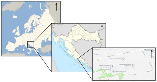
Figure 4.
The University of Split Campus in the city of Split, Republic of Croatia.
Given that fuzzy logic is based on modeling expert knowledge, the involvement of experts in defining and implementing the MB is crucial. A group of experts included 4 experts from the Faculty of Civil Engineering, Architecture and Geodesy of University of Split, 2 experts from the University of Split, and 3 experts from the Faculty of Geodesy of University of Zagreb dealing with spatial planning, land management, and land systems. The first step of brainstorming with the experts included the selection of the method for cadastral parcels bonitet valuation. The next step was spatial analysis of the project area in order to identify a set of cadastral parcels and define criteria for their comparison.
3.2. Implementation Procedures
Spatial analysis is defined by the urban plan of the Campus project. The result is identification of 62 private cadastral parcels in the research area.
Step 1—Defining criteria for cadastral parcels comparison (input data), linguistic variables, and terms (initial phase)
The definition of cadastral parcels set and their initial analysis identified the criteria (input variables) used in their comparison. The final set includes the seven input variables (Figure 2). Given that cadastral parcels share some of the same spatial properties, the set of criteria is reduced for those related to location and infrastructural characteristics (microlocation, aspect, infrastructure, ecology, and vegetation). Figure 5 shows the general structure of the fuzzy logic model; the left shows the defined seven criteria as input variables and the right shows the output variable (the bonitet assessment).
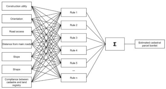
Figure 5.
Input and output variables to estimate of cadastral parcel bonitet.
Step 2—Cadastral parcels evaluation by all criteria
By determining the ideal shape of the cadastral parcel, the deviation of each cadastral parcel from its ideal shape according to the criteria selected for their comparison was determined. The difference is defined by a crisp number, but before determining the fuzzy input values, and in order to compare cadastral parcels according to the criteria of different character, it is necessary to carry out their standardization, i.e., reduction to the relation from 0 to 1.
Step 3—Normalization of input data—linear and value functions (input data—“crisp” input)
The input variables (criteria for comparing cadastral parcels) are defined below, and linear and nonlinear (value) functions are determined for the purpose of the standardization procedure. Standardization is carried out for the purpose of definition of input variables values in the range from 0 to 1 which allows their comparison.
Construction utility
The criterion is determined by the official data of the cadastre and land register, and its standardization is defined based on data for the size and construction of the building parcel for the area of the City of Split. Section 2.2.1.1. Paragraph 15 of the Official Gazette of the City of Split [32] defines the minimum sizes of building parcels for construction in the urban area. Based on the minimum values prescribed by the Official Gazette and expert assessment, the classes of cadastral parcels evaluation are defined:
1 st class: cadastral parcels whose area does not exceed 200 m2. The upper limit is defined in accordance with the provisions in the Official Gazette on the minimum size of the cadastral parcels for buildings that are built in a row,
2 nd class: cadastral parcels with an area in the range of 200 to 400 m2. The boundaries are defined in accordance with the provisions on the minimum size of the cadastral parcel: the lower limit for the buildings in the row (minimum parcel area is 200 m2) and the upper limit for free-standing buildings (minimum parcel area is 400 m2).
3 rd class: cadastral parcels with an area in the range of 400 to 1000 m2,
4 th class: cadastral parcels with an area in the range of 1000 to 2000 m2,
5 th class: cadastral parcels with an area of more than 2000 m2.
Standardized values of construction utility are defined by a linear transformation of the area of cadastral parcels and are given in the range from 0 (cadastral parcels that are not constructionally usable) to 1 (cadastral parcels whose area exceeds 2000 m2) and are shown by the graph in Figure 6.
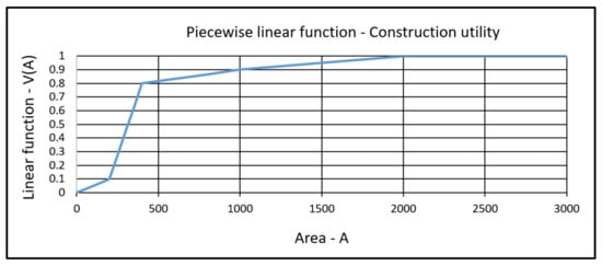
Figure 6.
Graph of a piecewise linear area function.
The graph shows five linear functions depending on the defined classes of cadastral parcels area. The linear transformation is defined for each class separately and is expressed by the formula ( is the area of the cadastral parcel j, is the linear function for the i class):
1st class:
2nd class:
3rd class:
4th class:
5th class:
Standardized area values are hereinafter referred to as .
Orientation
The criterion was determined based on slope orientation data for each cadastral parcel towards the sides of the world (showing slope exposure towards N, NE, E, SE, S, SW, W, NW, and flat areas) obtained by the Aster digital relief model analysis. The value of each cell in the output grid defines the direction in which the slope faces each side of the world. It is measured in degrees clockwise from 0° (north direction) to 360° (again north direction). Flat surfaces without slope are given a value of −1. In Table 1, the sides of the world with defined value ranges [33] are shown.

Table 1.
Ranges of slope orientation values towards the sides of the world [33].
Values of orientation are standardized using a fourth-order polynomial value function defined by the expression ( is the orientation of cadastral parcel j, and is the value function defined for the orientation):
Standardized orientation values are given in the range from 0 to 1, where grade 1 is defined for the south direction, i.e., 180° within the class south, and grades 0 for the north direction, i.e., 0° to 22.5° and 337.5° to 360° within class north. Grades of 0.5 were assigned to the east (90°) and west (270°) directions.
In Figure 7, a graphical representation of the specified function is given.
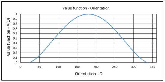
Figure 7.
Graph of the value function of the orientation.
Standardized orientation values are hereinafter referred to as .
Road access
Access to the registered road is defined by a binary evaluation of the criteria:
- -
- cadastral parcels that have access to a registered road are assigned a grade of 1.
- -
- cadastral parcels that do not have access to a registered road are assigned a grade of 0.
As this is a criterion for evaluating cadastral parcels with two crisp grades (0 and 1), only two MFs are defined, which is a case that is very rarely applied when defining the functions of input variables. It is known that for less than three MFs it is not possible to differentiate the set. However, the experts decided to include this criterion because the absence of the same would not result in a complete analysis and objective approach when comparing cadastral parcels.
Distance from main roads
The distance from the main roads is determined as the shortest distance of the cadastral parcels to one of the four main streets: Matica Hrvatska, Vukovarska Street, Bruno Bušića Street, and Velebitska Street, and it is expressed in meters. Given the linear character of the criteria values, for the purposes of their standardization the linear transformation was defined. The distance from the main roads is defined from 0 to 1 as a criterion of minimum, i.e., grade 1 is given to cadastral parcels whose distance from the road is 0 m, while grade 0 is given to t cadastral parcels that are 1000 meters and more away from roads. The linear function of the distance from the main roads is defined by the expression ( is the distance from the main road of the cadastral parcel j, and is the linear function defined for the distance):
In Figure 8, a graphical representation of the linear function for the specified criterion is shown.
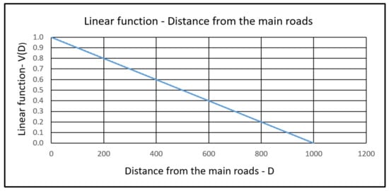
Figure 8.
Graph of the linear function of the distance from the main roads.
Standardized values of distance from main roads are hereinafter referred to as .
Slope
The criterion was determined based on terrain slope data for each cadastral parcel obtained by analysis of the Aster digital relief model and it is expressed in degrees. Given the linear character of the criteria values, for the purposes of their standardization the linear transformation was defined. The slope is defined from 0 to 1 as a criterion of minimum, i.e., grade 1 is given to cadastral parcels that have a slope from 0° to 2°, while grade 0 is given to those cadastral parcels that have a slope of 33° and more. The linear slope function is defined by the expression ( is the slope of the cadastral parcel j, and is the expression for the linear function):
In Figure 9, a graphical representation of the linear slope function is shown.
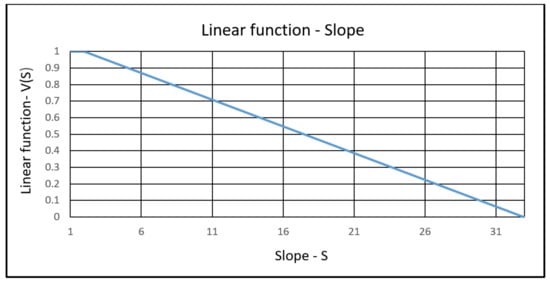
Figure 9.
The graph of the linear slope function.
Standardized slope values are hereinafter referred to as .
Shape
The shape of the cadastral parcel was determined based on three independent, one-parameter indices: the index of compactness, the index of rugosity, and the index of boundary points. The choice of criteria is the same as for agricultural land (proposed in the doctoral dissertation of Iva Odak [34]) with the difference in the choice of the cadastral parcel optimal shape. For an urban area, a solid with all equal sides (a square) is defined as the optimal cadastral parcel shape. Although the shape of the cadastral parcel is determined by the urban plan and the parameters defined in the plan should be taken in a more detailed assessment, to identify general guidelines to assess the cadastral parcels bonitet, the square was chosen as the most favorable form for building on it.
Compactness is determined by the expression [35]
where is area of the cadastral parcel j, the is the circumference of the cadastral parcel is j, and the compactness is expressed in the range of values from 0 to 1 (compactness of the circle).
As the optimal shape of the cadastral parcel in urban areas is equal to a square with a side ratio of 1:1, it is necessary to standardize the function in such a way that its maximum value is defined for the compactness of the square that is .
The compactness values are standardized using a sixth-order polynomial value function defined by the expression ( is the compactness of the cadastral parcel j and is the value function defined for compactness):
Standardized values, as well as values before standardization, are defined by an absolute grade ranging from 0 (cadastral parcels of the most unfavorable shape) to 1 (cadastral parcels of square shape). Standardized values of compactness are graphically shown in Figure 10 and are hereinafter referred to as the index of compactness.
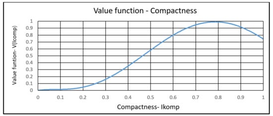
Figure 10.
Graph of the value function of cadastral parcel compactness.
Rugosity is defined as the ratio of the circumference of a cadastral parcel convex hull, which represents the smallest circumference of a solid and the circumference of that same cadastral parcel and is defined by the expression [36]
where is the circumference of the convex hull of the cadastral parcel j, the circumference of the cadastral parcel j, and the index of rugosity of the cadastral parcel j.
The rugosity values are defined in the range 0 to 1, where grade 1 represents those cadastral parcels whose circumference is equal to the circumference of the convex hull (cadastral parcels with optimal circumference).
The number of boundary points is determined based on defining the optimal number of points (sides) of the cadastral parcels and defining their standardized function. The optimal number of points is defined concerning the optimal shape of the cadastral parcel that is equal to a square. Accordingly, the optimal number of boundary points is equal to 4.
The number of boundary points are standardized using a fifth-order polynomial value function defined by the expression ( is the number of boundary points of the cadastral parcel j, and is the value function defined for the number of boundary points) [37]:
Standardized values of the number of boundary points are graphically shown in Figure 11.
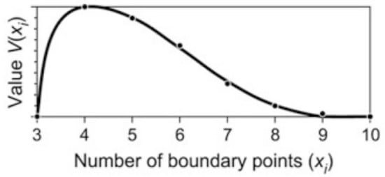
Figure 11.
Graph of number of boundary points value function [37].
The index of shape is ultimately defined as the arithmetic mean of the three listed indices:
where is the index of compactness of the cadastral parcel j, is the index of rugosity of the cadastral parcel j, and is the number of boundary points of the cadastral parcel j. The values of the index of shape are defined in the range from 0 to 1, where grade 1 represents cadastral parcels with optimal shape (square shape), while 0 is assigned to cadastral parcels of extremely irregular shapes.
In Table 2 the values of the index of compactness, index of rugosity, index of the number of boundary points, and the index of shape are shown. For the sake of transparency, the indices are shown for 10 of 62 cadastral parcels.
Table 2.
Index of compactness, index of rugosity, index of the number of boundary points, and the index of shape.
Compliance between cadastre and land registry
The compliance of the cadastre and the land register is defined by a binary evaluation of the criteria:
- -
- Cadastral parcels for which the data in the cadastre and land register are harmonized have been assigned a grade of 1.
- -
- Cadastral parcels for which the data in the cadastre and land register are not harmonized were assigned a grade of 0.
As is the case with the road access criteria, cadastral parcels are evaluated with two crisp grades, 0 and 1, and accordingly, two MFs are defined with clear, crisp boundaries of belonging to a particular set (cadastral parcels belongs or does not belong to a particular set).
The evaluation of cadastral parcels was performed according to the defined criteria and is shown in Table 3. For the sake of transparency, the evaluation is shown for 10 of 62 cadastral parcels.
Table 3.
Standardized results of cadastral parcels.
Step 4—Defining MFs
A triangular MF has been selected to define the membership of the input variables. The shape, number, and range of MFs of input and output variables are shown below.
Construction utility
The input variable construction utility is defined with six MFs depending on the classes of construction utility evaluation of cadastral parcels shown in step number 3. In Table 4, fuzzy sets of construction utility and their associated linguistic values are presented.
Table 4.
Defining fuzzy sets and values of the linguistic variable “Construction utility”.
In Figure 12, the shape, number, and range of MFs for the construction utility criterion are presented.
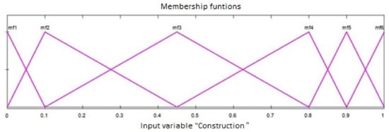
Figure 12.
MFs of the input variable “Construction utility”.
Orientation
The input variable orientation is defined by five uniformly distributed MFs with the degree of overlap depending on the value function of the cadastral parcel orientation shown in step 1. In Table 5, fuzzy sets of cadastral parcels orientation and their associated linguistic values are presented.
Table 5.
Defining fuzzy sets and values of the linguistic variable “Orientation”.
In Figure 13, the shape, number, and range of MFs for the orientation criterion are presented.
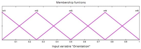
Figure 13.
MFs of the input variable “Orientation”.
Road access
The input variable road access is defined with two functions representing two crisp sets. In Figure 14 the shape, number, and range of MFs for the input variable road access are shown.
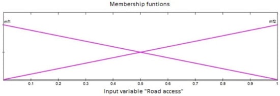
Figure 14.
MFs of the input variable “Road access”.
Distance from main roads
The input variable distance from the main roads is defined with six uniformly distributed MFs with the degree of overlap . In Table 6, fuzzy sets and their associated linguistic values are shown.
Table 6.
Defining fuzzy sets and values of the linguistic variable “Distance from the main road”.
In Figure 15, the shape, number, and range of MFs for the distance from the main roads criterion are presented.
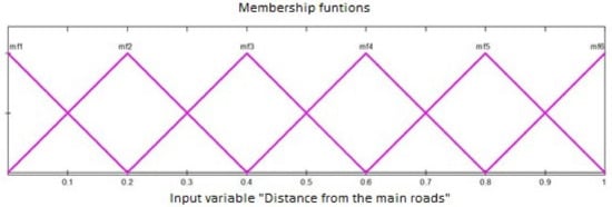
Figure 15.
MFs of the input variable “Distance from the main roads”.
Slope
The input variable slope is defined with seven MFs depending on the value function of the cadastral parcel slope shown in step 3. In Table 7, fuzzy sets of cadastral parcels slope and their associated linguistic values are shown.
Table 7.
Defining fuzzy sets and values of the linguistic variable “Slope”.
In Figure 16, the shape, number, and range of MFs for the slope criterion are presented.
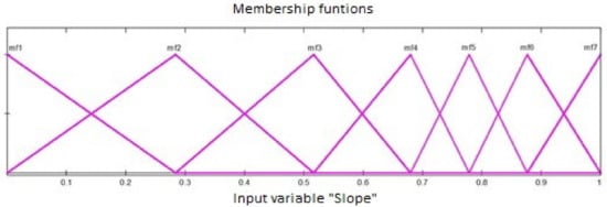
Figure 16.
MFs of the input variable “Slope”.
Shape
The input variable shape, as well as the distance from the main roads, is defined with six uniformly distributed MFs with the degree of overlap . In Table 8, fuzzy sets and their associated linguistic values are shown.
Table 8.
Defining fuzzy sets and values of the linguistic variable “Shape”.
In Figure 17, the shape, number, and range of MFs for the shape criterion are presented.
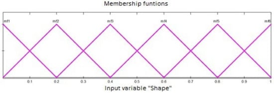
Figure 17.
MFs of the input variable “Shape”.
Compliance between cadastre and land registry
The input variable compliance between cadastre and land registry is defined with two functions representing two crisp sets. In Figure 18, the shape, number, and range of MFs for the input variable compliance between the cadastre and land registry are shown.
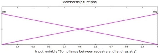
Figure 18.
MFs of the input variable “Compliance between cadastre and land registry”.
Bonitet
The output variable bonitet of the cadastral parcels is defined with eleven uniformly distributed MFs with a degree of overlap . In Table 9, fuzzy sets of bonitet and their associated linguistic values are presented. The reason for choosing a larger number of output fuzzy sets is the need for greater accuracy of the output data when comparing cadastral parcels with small differences in the attribute values of the input variables.
Table 9.
Defining fuzzy sets and values of the linguistic variable “Bonitet”.
In Figure 19, the shape, number, and range of MFs for the output variable bonitet are shown.
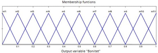
Figure 19.
MFs of the output variable “Bonitet”.
Step 5—Defining the rule base in the knowledge base
As already mentioned, the development of a rule base is a complex and time-consuming process. The total number of rules that need to be defined within this research is
Given the large number of rules that need to be defined, as well as the impossibility of maintaining consistency when defining the relationships of their causal and consequential relations, the methodology used to mathematically define the logical relationship of input and output variables was applied in creating the rule base. The advantage of the proposed methodology is primarily found in maintaining consistency in defining the rules, and then in facilitating and accelerating expert assessment. In contrast to the traditional approach to defining rules based on individual expert assessment of the input–output relationship in logical equations, by application of this methodology expert knowledge was primarily used to define weights, which on the one hand took into account the relative ratio of input variables, and on the other hand defined their association with the output variable. Using the AHP method, the weights (W) of the input variables were defined by expert evaluation. Further, the consistency ratio was determined, CR < 0.1, and for each expert, criteria weights satisfied this condition. In Table 10, their mean values determined by the arithmetic mean are shown. Averaging by the arithmetic mean was primarily chosen because in such a defined result all input values are equally represented. After defining the weight mean values, their percentage normalization (W ‘) was performed. The distribution of the weighting coefficient value according to the number of membership functions of the output variable (seven MFs) determines the relationship between the individual causal part of the logical equation and its consequences, i.e., its bonitet value. After the elimination procedure, which includes the elimination of rules that do not correspond to the defined data set and the elimination of redundant rules, the rules were reduced to 861. Table 10 shows a part of the rules that are associated with cadastral parcel 6505/1, i.e., the MFs of its input and output variables.
Table 10.
Part of fuzzy rules with a definition of weighting coefficients (cadastral parcel 6505/1).
Step 6—Conversion of input data crisp values into fuzzy values using MFs (fuzzification)
In the process of fuzzification, fuzzy values are assigned to the input crisp values. Fuzzy sets are described by triangular MFs, i.e., for each given crisp value are two fuzzy values. Each input value has got the sum of the membership degrees equal to one. Input values which membership is defined only by one fuzzy set are called singleton set (they membership to that set is one hundred percent, i.e., ). Singleton sets of input variables are
- -
- Construction utility:
- -
- Orientation:
- -
- Distance from the main roads:
- -
- Slope:
- -
- Shape:
The membership of cadastral parcels for the input variables “Road access” and “Compliance of cadastre and land registry” is defined with two singleton sets (cadastral parcels belong to either one or the other set).
Steps 7–9—Mamdani Fuzzy Inference System
The Mamdani model of local fuzzy inference was used to implement the fuzzy logic model. In the first step of the implementation, the interference operator is selected, i.e., the logical operator T-norm, by which the connection in the logical equations is defined by the intersection of the input variables MFs. The “AND” logical minimum operator is selected because it best defines the character of the input variables. In the second step of the reasoning process, the Mamdani implicator, i.e., the minimum operator, was applied. Accordingly, the resultant value of the causal part of the equation always corresponds to the minimum value of the input variables membership degrees (Step 7).
Clipping method was chosen to define the output fuzzy set. The conclusion of each equation is cut to a height determined by the minimum membership degree of the input variables. By applying the aggregation operator, all output fuzzy sets were combined into a single fuzzy set. For the decision operator, which includes the implication and aggregation operators, the Mamdani decision operator is selected, i.e., the max-min operator. The resultant value is defined as the union of previously defined segments of all fuzzy sets of one output variable (Step 8).
The conversion of the resulting output fuzzy values into their crisp numerical values is called the process of defuzzification, i.e., process of sharpening (Step 9). Defuzzification is performed by the center of gravity method (centroid method).
Step 10—Output data set (“crisp” estimated bonitet value of cadastral parcels)
By determining the ideal shape of the cadastral parcel (parcel with a bonitet value of 1), the deviation of each cadastral parcel from their ideal shape was determined according to the criteria selected for their comparison. The difference is defined by crisp number, i.e., bonitet value in the range from 0 (lowest bonitet value) to 1 (highest bonitet value). The bonitet values for all private cadastral parcels in the project area of the Campus, University of Split are shown in Table 11.
Table 11.
Bonitet values of private cadastral parcels.
Values of the private cadastral parcels bonitet values in the project area of the Campus, University of Split range from BV (6528/8) = 0.354 as the minimum value (smallest bonitet value) to BV (6566/2) = 0.900 as the maximum value (highest bonitet value). Most cadastral parcels, more precisely 52 of 62, have a bonitet value greater than 0.5 (84% of all parcels). The obtained bonitet values will be used for land reallocation in Urban Renewal process.
In Figure 20, the distribution of private cadastral parcels in the project area of the Campus, University of Split with their bonitet values is shown. Light red tones show those cadastral parcels with relatively small bonitet values, while dark red tones indicate the best rated cadastral parcels according to defined criteria (with the highest bonitet values).
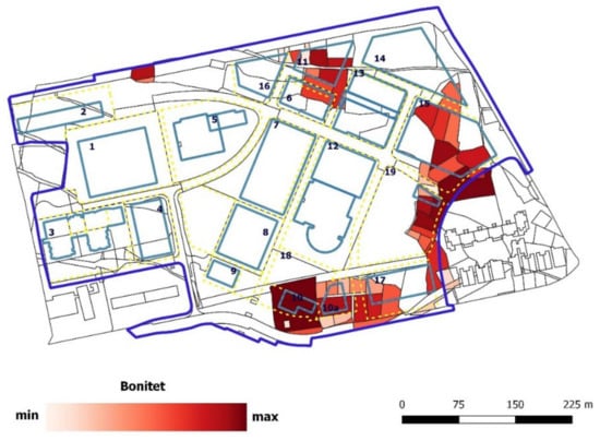
Figure 20.
Bonitet values of private cadastral parcels in the project area of the University of Split Campus.
4. Conclusions
In this paper, the authors proposed the calculation of bonitet as an assessment of cadastral parcels when defining the reallocation procedure in the urban renewal of a particular area. The final, 4th phase in planning the implementation of the urban renewal includes reallocation processes within a reallocation model (MR) that integrates the model to assess the bonitet of cadastral parcels (MB), the real estate valuation model (MRE), and the preferences of private parcels owners. MB, which is the subject of this research, was realized as an ES based on the principle of fuzzy logic within the knowledge component.
Initially, it is important to emphasize its difference in relation to the bonitet of agricultural land, which is defined in Croatian law through the Ordinance of standards for the determination of particularly valuable land for cultivation (P1) and the valuable agricultural land (P2). In the process of valuing agricultural land, to optimize the procedure, cadastral parcels are classified according to similar properties to assess their (bonitet) value. Criteria that may affect the value of the agricultural land are soil quality, climate, relief, and certain other conditions for agricultural production (location, its distance from the farmyard, built road, etc.). Certified appraisers perform the land valuation. The whole procedure is based on expert assessment, while the boundaries of individual classes are expressed unambiguously by a sharp, binary membership to sets (an individual cadastral parcel either belongs or does not belong to an individual set). Although the process is accelerating by classifying cadastral parcels, the main problem arises when it is necessary to determine the optimal number of classes. There is often a problem that expert decisions are ambiguous even after the agreement, and the aforementioned problem cannot be defined by a simple mathematical expression. The question is: what is the optimal number of classes for the classification of parcels, while maintaining the accuracy when comparing them? The main problem is the sharp bounds of the classes which often result in the classification of parcels with small numerical differences into two classes, while parcels with much larger numerical differences are sometimes classified into the same class. This affects the loss of precision while comparing them. Likewise, simple mathematical estimation systems do not have the ability to fine-tune changes in cadastral parcel attribute changes as well as their mutual interactions. A large number of influential elements results in complex and incomplete knowledge of experts and the impossibility of systematic consideration of the problem. Conditions that change depending on alternations in the cadastral parcel attribute values prevent its stochastic description. A frequent case is the insufficient number of recorded input data required for the quality implementation of quantitative analysis, the results of which depend only on the modeling of the data ratio of the available input set. Based on the above, there is a need to apply a model built on the experience of experts that offers the possibility of detailed description and analysis of complex interactions between input and output data.
This approach of classifying cadastral parcels could also be applied to the valuation of urban land, with the establishment of specific criteria for each task. However, based on these shortcomings, and taking into account the fact that the valuation of urban land (during urban renewal) is a much more specific procedure than the valuation of agricultural land, this study proposed an approach to objectify the process while increasing the accuracy of valuation.
To realize these requirements, an expert system based on fuzzy logic was selected. Its central part is its knowledge base, which was created based on expert assessment of the impact of different input variables (cadastral parcel attributes) on the output variable (expressed in the form of logical rules in the rule base). Given the complexity of the procedure due to a large number of input variables and the extensive rule base, the procedure was optimized by introducing weighting coefficients to shorten the time of defining the rule base, as well as maintaining consistency when defining rules of many different combinations of input variables and output variable fuzzy sets. A set of linear functions and nonlinear value functions for standardizing the ratings of alternatives for the seven defined comparison criteria. Defining weighting coefficients for optimizing the rule base and linear functions and nonlinear value functions for standardizing demonstrate how expert knowledge is included in the evaluation process. By applying the newly formed ES in the bonitet assessment, with the created base of expert knowledge, the processes of estimating attribute values have been improved, especially in the form of reducing estimation uncertainty (crisp class boundaries are replaced by fuzzy boundaries, as well as increasing objectivity by involving more experts in research).
The initial questions were confirmed and the final conclusions were given:
1. Is it possible to develop a model that will provide an approach to the valuation of existing urban land parcels, with a view to a fairer reallocation process?
The authors proposed a unique model of urban land valuation for the purpose of implementing the reallocation process in urban renewal. A review of the existing scientific and professional literature did not find a procedure that would be applicable in its original or modified form during the implementation of urban consolidation (or its specific form of urban renewal). The conclusion was that there is still no system that would provide support in solving such a complex task. MB was realized as a fuzzy expert system. The advantages of fuzzy logic are the ability to monitor small changes of input parameters and their interactions based on the expert definition of membership functions and inference rules that logically connect input and output data. The output crisp value is one of the data based on which a plan for reallocating private owners is proposed and adopted. The proposed approach provides a fairer allocation of private owners because each stakeholder can gain insight into the whole process thus gaining confidence in the protection of their property rights.
2. Is it possible to develop a flexible model that will be able to adapt to another research area?
The proposed model is flexible because it allows adaptation to a specific task. Apart from urban renewal, it can also be used in land valuation and in other specific urban consolidation procedures, as well as in the valuation of agricultural land. The logic of the model allows easy addition or removal of certain criteria as well as modification of the knowledge base with respect to a specific problem. If there is a requirement to expand the whole system, experts from the field of research should be included in the modification of the knowledge base again.
3. Is it possible to increase objectivity when adopting a reallocation plan?
The proposed model primarily provides an opportunity for an objective approach to the problem, which is achieved by involving a group of experts in the field of research, reducing uncertainty in the evaluation of urban land parcels, and giving equal access to each stakeholder in the urban renewal process.
By satisfying the set supportive questions/goals, it can be concluded that the hypothesis has been confirmed. The proposed approach provide the improvement of urban renewal planning by appropriate design of the model to assess the bonitet of cadastral parcels based on fuzzy expert system. Future research will certainly go in the direction of developing an overall reallocation system that will suggest an interaction between model to assess the bonitet of cadastral parcels (MB), the real estate valuation model (MRE), and the preferences of private parcels owners. Each of these components has been developed separately, but the task remains on the development of a system that will automatically propose a future urban spatial plan. Equally, the collection of preferences of private owners would go in the direction of developing the application in which they would, in addition to insight into the current situation and appraisal of their own real estate, express their own preferences by accessing the created questionnaire. The development of large public projects is most often realized over many years, so in addition to the spatial component, it is necessary to include the time component in the entire system. Real estate values change over time, so the question arises as to how to propose allocation plans: before the start of urban renewal or at different time intervals? Kilic et al. proposed a methodology when valuing agricultural land, but there is certainly space left for the development of system components that would be applicable during agricultural land consolidation (integration of preferences of private owners, real estate valuation, and bonitet of cadastral parcels).
Author Contributions
Conceptualization, J.K.P., K.R., and N.J.; methodology, J.K.P., K.R., and N.J.; software, J.K.P., K.R., and N.J.; validation, J.K.P., K.R., and N.J.; formal analysis, J.K.P., K.R., and N.J.; investigation, J.K.P., K.R., and N.J.; resources, J.K.P., K.R., and N.J.; data curation, J.K.P., K.R., and N.J.; writing—original draft preparation, J.K.P., K.R., and N.J.; writing—review and editing, J.K.P., K.R., and N.J.; visualization, J.K.P., K.R., and N.J.; supervision, J.K.P., K.R., and N.J.; project administration, J.K.P., K.R., and N.J.; funding acquisition, J.K.P., K.R., and N.J. All authors have read and agreed to the published version of the manuscript.
Funding
This research received no external funding.
Institutional Review Board Statement
Not applicable.
Informed Consent Statement
Not applicable.
Data Availability Statement
Data available on request due to restrictions eg privacy or ethical. The data presented in this study are available on request from the corresponding author. The data are not publicly available due to further research to be published.
Acknowledgments
This research is partially supported through project KK.01.1.1.02.0027, a project co-financed by the Croatian Government and the European Union through the European Regional Development Fund—the Competitiveness and Cohesion Operational Programme.
Conflicts of Interest
The authors declare no conflict of interest.
References
- Simpson, W. Report to the Minister for Local Government and Minister for Planning on an Inquiry Pursuant to Section 119 of the EPAA with Respect to REP 12, SEPP 5 and SEPP 25; NSW Parliamentary Library: Sydney, Australia, 1989. Available online: http://friendsoftuggerahlakes-cen.org.au/TEPCP/TEPPS%20RESEARCH%20PAPERS/Urban%20Consolidation%20Current%20Developments%2023-97.pdf (accessed on 30 November 2020).
- Yanase, N. Understanding Kukaku-Seiri (land readjustment). Conference Paper on JICA’s Urban Development Course. 2013, Japan. Available online: https://www2.ashitech.ac.jp/civil/yanase/lr-system/UNDERSTANDING%20KUKAKU.pdf (accessed on 30 November 2020).
- Hong, Y.H.; Brain, I. Land Readjustment for Urban Development and PostDisaster Reconstruction. Land Lines 2012, 24, 2–9. [Google Scholar]
- Rahnama, R.M.; Akbari, M. Analysis the Status of Land Readjustment (LR) in Urban Development of Iranian Cities, A Case of Gonabad Neighborhood Garden. Mediterr. J. Soc. Sci. 2016, 7, 301–305. [Google Scholar] [CrossRef]
- Kilić, J. Modelling Spatial Decision Support System to Planning of Urban Land Consolidation. Mater’s Thesis, University of Zagreb, Zagreb, Croatia, 2019. [Google Scholar]
- Kilić, J.; Rogulj, K.; Jajac, N. Fuzzy Expert System for land valuation in land consolidation processes. Croat. Oper. Res. Rev. 2019, 10, 89–103. [Google Scholar] [CrossRef]
- Official Gazette 151/2013. Ordinance of standards for the determination of particularly valuable land for cultivation (P1) and the valuable agricultural land (P2), Republic of Croatia. Available online: https://narodne-novine.nn.hr/clanci/sluzbeni/2013_12_151_3201.html (accessed on 30 November 2020).
- Kilić, J.; Jajac, N.; Rogulj, K.; Mastelić-Ivić, S. Assessing Land Fragmentation in Planning Sustainable Urban Renewal. Sustainability 2019, 11, 2576. [Google Scholar] [CrossRef]
- Branković, S.; Parezanović, L.; Simović, D. Land consolidation appraisal of agricultural land in the GIS enviroment. Geod. Vesn. 2015, 59, 320–334. [Google Scholar]
- Demetriou, D.; Stillwell, J.; See, L. An integrated planning and decision support system (IPDSS) for land consolidation: Theoretical framework and application of the land-redistribution modules. Environ. Plan. B Plan. Des. 2012, 39, 609–628. [Google Scholar]
- Uyan, M.; Cay, T.; Akcakaya, O. A Spatial Decision Support System design for land reallocation: A case study in Turkey. Comput. Electron. Agric. 2013, 98, 8–16. [Google Scholar] [CrossRef]
- Cay, T.; Uyan, M. Evaluation of reallocation criteria in land consolidation studies using the Analytic Hierarchy Process (AHP). Land Use Policy 2013, 30, 541–548. [Google Scholar] [CrossRef]
- Zou, X.; Luo, M.; Su, W.; Li, D.; Jiang, Y.; Ju, Z.; Wang, J. Spatial decision support system for the potential evaluation of land consolidation projects. WSEAS Trans. Comput. 2008, 7, 887–898. [Google Scholar]
- Cay, T.; Ayten, T.; Iscan, F. An investigation of reallocation model based on interview in land consolidation. In Proceedings of the 23rd FIG Congress, Shaping the Change, Munich, Germany, 8–13 October 2006. [Google Scholar]
- Cay, T.; Iscan, F. Determination of land piece given to farmers in land reform by using the fuzzy logic method. In Proceedings of the 23rd FIG Congress, Shaping the Change, Munich, Germany, 8–13 October 2006. [Google Scholar]
- Cay, T.; Iscan, F. Application of fuzzy logic in land consolidation activities. In Proceedings of the XXIV International FIG Congress, Sydney, Australia, 11–16 April 2010. [Google Scholar]
- Cay, T.; Iscan, F. Fuzzy expert system for land reallocation in land consolidation. Expert Syst. Appl. 2011, 38, 11055–11071. [Google Scholar] [CrossRef]
- Kagita, M.K.; Tata, H.K.; Manava, A.C. A fuzzy environment strategies for optimal agricultural land allocation in Krishna delta. IRJCS Int. Res. J. Comput. Sci. 2018, 5, 57–64. [Google Scholar]
- Ertunç, E.; Cay, T. Application of Fuzzy Logic in Land Consolidation-Classification Studies. Intell. Syst. Appl. Eng. 2016, 4, 118–123. [Google Scholar] [CrossRef][Green Version]
- von Altrock, C. Fuzzy Logic and Neurofuzzy Applications Explained; Prentice-Hall Inc.: Upper Saddle River, NJ, USA, 1995. [Google Scholar]
- Bonato, J.; Skendorović, J. Regulacija rada dizalice pomoću fuzzy logike. Pomor. Zb. Poseb. Izd. 2016, 273–281. [Google Scholar] [CrossRef]
- Zadeh, L.A. Fuzzy Sets. Inf. Control 1965, 8, 338–353. [Google Scholar] [CrossRef]
- Ross, T.J. Fuzzy Logic with Engineering Applications; John Wiley & Sons Ltd.: West Sussex, UK, 2004. [Google Scholar]
- Demetriou, D. The Development of an Integrated Planning and Decision Support System (IPDSS) for Land Consolidation. Mater’s Thesis, University of Leeds, Leeds, UK, 2014. [Google Scholar]
- Beinat, E. Value Functions for Environmental Management; Kluwer Academic Publishers: Dordrecht, The Netherlands, 1997. [Google Scholar]
- Zarandi, M.H.F.; Mohammadhasan, N.; Bastani, S. A Fuzzy Rule-Based Expert System for Evaluating Intellectual Capital. Adv. Fuzzy Syst. 2012, 2012, 823052. [Google Scholar] [CrossRef]
- Šitum, Z. Regulacija Pneumatskog Servosustava Primjenom Neizrazitog Regulatora. Mater’s Thesis, University of Zagreb, Zagreb, Croatia, 2001. [Google Scholar]
- Lončar, D. Fuzzy Logic Application in Thermal Power Plant Control System. Mater’s Thesis, University of Zagreb, Zagreb, Croatia, 2001. [Google Scholar]
- Nandi, K.A. GA-Fuzzy Approaches: Application to Modeling of Manufacturing Process. In Statistical and Computational Techniques in Manufacturing; Springer: Berlin/Heidelberg, Germany, 2013; pp. 145–185. [Google Scholar]
- Runkler, T. Selection of appropriate defuzzification methods using application specific properties. IEEE Trans. Fuzzy Syst. 1997, 5, 72–79. [Google Scholar] [CrossRef]
- Saaty, T.L. Fundamentals of Decision Making and Priority Theory with the Analytic Hierarchy Process; RWS publications: Pittsburgh, PA, USA, 2000; Volume 6. [Google Scholar]
- Official Gazette of the City of Split. Available online: http://www.split.hr/lgs.axd?t=16&id=162 (accessed on 30 November 2020).
- Esri. Available online: https://www.esri.com/arcgis-blog/products/product/mapping/aspect-slope-map/ (accessed on 30 November 2020).
- Odak, I. Agricultural Land Fragmentation Analysis of Land Holdings and its Application in the Rural Land Management. Mater’s Thesis, University of Zagreb, Zagreb, Croatia, 2017. [Google Scholar]
- Osserman, R. Isoperimetric inequality. Bull. Am. Math. Soc. 1978, 84, 1182–1238. [Google Scholar] [CrossRef]
- Chan, A.H.S.; So, D.K.T. Measurement and quantification of visual lobe shape characteristics. Int. J. Ind. Ergon. 2006, 36, 541–552. [Google Scholar] [CrossRef]
- Demetriou, D.; Stillwell, J.; See, L. A new methodology for measuring land fragmentation. Comput. Environ. Urban Syst. 2013, 39, 71–80. [Google Scholar] [CrossRef]


Publisher’s Note: MDPI stays neutral with regard to jurisdictional claims in published maps and institutional affiliations. |
© 2020 by the authors. Licensee MDPI, Basel, Switzerland. This article is an open access article distributed under the terms and conditions of the Creative Commons Attribution (CC BY) license (http://creativecommons.org/licenses/by/4.0/).