Abstract
In the eastern Democratic Republic of Congo, agriculture represents the most important economic sector, and land control can be considered a perpetual source of conflict. Knowledge of the existing production system distribution is fundamental for both informing national land tenure reforms and guiding more effective agricultural development interventions. The present paper focuses on existing agricultural production systems in Katoyi collectivity, Masisi territory, where returning Internally and Externally Displaced People are resettling. We aim to define a repeatable methodology for building evidence-based and updated knowledge concerning the spatial distribution of the two existing production systems: subsistence-oriented agriculture (SOA) and business-oriented agriculture (BOA). To this aim, we used a supervised object-based classification approach on remotely sensed Sentinel-2 imagery to classify land cover. To classify production systems further within the “agriculture” and “pasture” land use classes, binary classification based on an entropy value threshold was performed. An iterative approach was adopted to define the final HNDVI threshold that minimised commission and omission errors and maximised overall accuracy and class separability. The methodology achieved acceptable observed accuracy (OA equal to 80–90% respectively for agricultural and pasture areas) in the assessment. SOA and BOA respectively covered 24.4 and 75.6% of the collectivity area (34,606 ha). The results conclude that land use and entropy analysis can draw an updated picture of existing land distribution among different production systems, supporting better-adapted intervention strategies in development cooperation and pro-poor agrarian land tenure reforms in conflict-ridden landscapes.
1. Introduction
The control of land has always been at the core of profound disputes in the Democratic Republic of Congo (DRC) [1,2,3]. The tragic series of events culminating in the Congolese war between 1994 and 2004 and the Tutsi Genocide, together with an ineffective state policy and a chronic insecurity situation, has led to the disruption of the agricultural sector and an increasingly intense conflict over access to land [4]. The historical background and varied orography of the Goma Diocese, located at the border between North and South Kivu provinces, has directly led to a complex agricultural landscape, with significant impacts on the natural environment and regional economic development [5,6]. The situation is further complicated by the massive number of Internally and Externally Displaced People (IDP and EDP, respectively); e.g., the OCHA estimated 863,400 IDPs between January 2009 and November 2014. According to existing international treaties, all these people have the right to return to their homes [7]. According to previous studies, socio-economic conditions profoundly influence terrestrial ecosystems, especially agroecosystems and their ability to support human settlements [8]. The agenda of international organizations dealing with peace-seeking and peacekeeping in the Eastern Congo now focuses on, among other issues, drawing a clear outline of land distribution among the different stakeholders in the agricultural sector [9,10]. Two different agricultural production systems exist in the region. These agricultural production systems are understood here as the two main types of livelihood strategies among the Congolese population of the Goma Diocese, namely Subsistence Oriented Agriculture (SOA) and Business Oriented Agriculture (BOA). The first is the type of agricultural activity defined as family farming by the FAO [11]. It is usually implemented on small plots of land, with access to very local markets. In DRC and specifically in the Goma Diocese, this production system forms a mosaicised land use/land cover (LULC) pattern that other authors identified as the “rural complex” [12,13]. The rural complex is a distinctive agricultural land cover mosaic surrounding the network of inhabited areas found along rivers and roads in DRC. It contains paths, grassy and bare communal areas, settlements and various land uses, primarily those associated with traditional smallholder livelihood shifting cultivation: cleared land, active fields, fallow fields, secondary forest and a permeable interface area with primary forest [12].
Conversely, huge plantations or grazing areas mostly characterise BOA, whose products are usually sold in foreign or regional markets. The two agricultural systems also differ in terms of land tenure, as SOA generally implies the exploitation of lands attributed to farmers through the traditional land tenure system and/or with no titling at all [11], while BOA usually relies on formally titled land. The two productive systems generate different costs and benefits for the local economy and existing socio-ecological systems [14,15,16]. In such a chronic emergency context, socio-economic development heavily depends on the resiliency of the agricultural sector [17]. Consequently, in-depth knowledge of regional agricultural geography is fundamental for understanding the spatial distribution and evolution of food supply chains, supporting the reintegration of IDPs/EDPs [18], and most of all assessing the impact of current and future policies and peacekeeping interventions [3,19,20].
To our knowledge, no official data exist regarding the spatial distribution of BOA and SOA systems in the Goma Diocese, especially at the scale of analysis of interest. In the DRC, and especially in the provinces of North and South Kivu, agriculture and livestock breeding constitute the backbone of socio-economic development [17]. Information regarding the distribution of land among the existing production systems is also fundamental for supporting advocacy actions towards the need for pro-poor land tenure reform in the DRC, which is debated since 2012 [21,22,23,24,25]. Given the characteristic inaccessibility of the territory, both in physical terms due to orography and insecurity, and in terms of data availability due to the lack of governmental official knowledge repositories, satellite remote sensing (RS) is a suitable option as an analysis tool. The present study aims to build evidence-based and updated knowledge regarding the spatial distribution of agricultural production systems in agricultural and pasture areas through land use analysis and entropy analysis of remote sensed Sentinel-2 imagery in the collectivity of Katoyi, North Kivu, DRC.
Although several previous studies tested the use of RS in the DRC [26,27,28], to the best of our knowledge, only two remote sensing-based LULC analyses focusing on the DRC exist [29,30], which present respectively a tiny scale of analysis and out-of-date information compared to our needs. Land use is strongly related to land cover, as the kind of activity implemented in a territory strongly depends on the features of the available environment and vice versa [31]. In the present study, we adopted the LULC acronym to focus on the functional definition of land use, which points to the description of the land in reference to its socio-economic purpose [32]. Therefore, LULC-change analyses can be of paramount importance for mapping the evolution of specific geographical contexts′ socio-economic activities. This possibility is more significant where livelihood agricultural systems and forest preservation objectives represent coexisting aims.
LULC change studies are widely accepted to be essential for enabling preventive actions against natural resource degradation and destruction [33], especially in inaccessible zones such as the Congolese basin. As previously mentioned, LULC maps can highlight borders between different socio-economic uses within a given territory. Nevertheless, without other auxiliary information layers, it hardly describes the territory according to a series of operations carried out by humans in order to obtain specific products and/or benefits. This means that land use, in its sequential definition, cannot be inferred directly from land cover [34].
To unmix LULC mapping information within a specific LULC class, an entropy-based approach and texture analysis of satellite imagery seems to be promising and widely used in the literature [35,36,37,38,39,40]. Texture is an intrinsic property of virtual surfaces, and can be defined as the expression of patterns in the spatial variation of pixel values in imagery, which contain essential information concerning the structural arrangement of surfaces and their relationship to the surrounding environment [41]. There are different metrics used as expressions of textural features, and entropy is one of them. This parameter measures an image’s disorder: if an image is not uniform in terms of texture, a high entropy value will characterise it [42]. Entropy and other textural features have been widely used in remote sensing with reasonably satisfactory results [43]; in particular, these features can be directly used for scene classification or to improve LULC classification accuracy by adding information to spectrum-related data [44]. RS has significant potential for applications in this respect, but considering that this study area is located in the equatorial belt, some limitations should also be pointed out. On average, rainfall is very abundant in equatorial and forested regions characterised by intense evapotranspiration [45]. Moreover, high mountains characterise the study area and the surrounding region. For this reason, the area is known for the strong presence of clouds [46], which makes it challenging to collect multiple contiguous optical observations, both spatially and temporally [47,48,49,50].
2. Materials and Methods
2.1. Study Area
The present research focuses on the Katoyi Collectivity, located in Goma Diocese (GD), North Kivu, Democratic Republic of Congo (DRC). The GD (surface: 26,223 km2) is located in the eastern DRC (DRC, Figure 1a,b). GD is an ecclesiastical administrative unit known as “small north” (“le petit Nord”). It is located in the North Kivu province and a small strip of the Kalehe Territory (Figure 1c) lying in the South Kivu province. Within the Diocese, there are 11 collectivities belonging to five territories (Goma, Rutshuru, Masisi, Walikale, and Kalehe). The study area is characterised by one of Africa’s highest population densities (2,211,000 inhabitants on 26,223 km2 of territory, 88.4 inhabitants/km2). A very high poverty level characterises the local population (72.9% of the population live below the UN poverty threshold in North Kivu, against 71.2% in the whole DRC) [51,52].
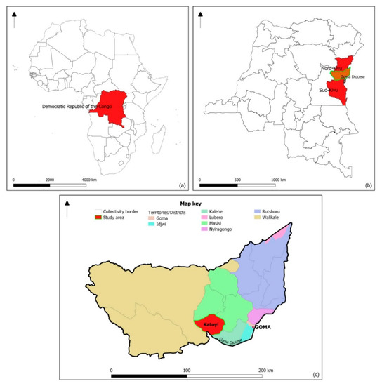
Figure 1.
Geographical framework of the study area. The Democratic Republic of the Congo (a); The Goma Diocese, located in the extreme east of the DRC, in North and South Kivu provinces (b); The collectivity of Katoyi, located at the south border of the Goma Diocese (c).
The GD’s orography is very complex. A continuous series of tiny plains, plateaus, hills and mountains make up the landscape. The local agricultural system can be framed in terms of the agroecological zones defined by FAO [53]: moving westward from the higher altitudes that lie along the borders with the neighbouring Uganda, Rwanda and Burundi and heading towards the forest, the farming system called “Highland Perennial” gives way to a “Forest-Based” system [53]. In this setting, the two previously mentioned production systems coexist. Small farmers mainly practice SOA, aiming at subsistence through family agriculture on small plots, mainly located near villages, on uplands officially under customary tenure or ad hoc agreements with private landowners. BOA is practised on or near large landholdings. It grows mainly cash crop plantations in monocultural cropping systems or breeds cattle in extensive systems [54]. Masisi territory and Katoyi collectivity, in particular, have been the theatre of massive population displacements from 1994 to 2004. During this period, the Katoyi collectivity hosted the headquarters of the leading armed group in the area at that time, the Democratic Forces for the Liberation of Rwanda [55]. Due to their presence, most of the population fled and left the collectivity scarcely inhabited during the following ten years. Since 2015, returning IDPs and EDPs have slowly resettled in the collectivity of Katoyi (according to unpublished CARITAS Development Goma reports of 2015).
2.2. Workflow
The present research firstly addresses the LULC of the GD in order to map the agricultural and pasture areas, and secondly assesses the existing agricultural production systems (i.e., SOA and BOA) in a strategic collectivity, i.e., Katoyi, in order to support rural development policies and programs. We review the proposed three-phase workflow in Figure 2.
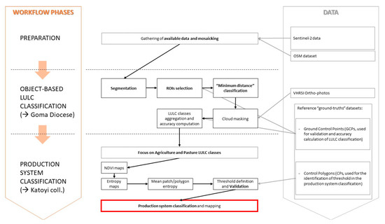
Figure 2.
Workflow showing the main operations for obtaining final results in LULC acquisition from S2 multispectral imagery.
During the preparation phase (see Figure 2), we collected and organised all relevant data in order to tackle spatial analysis by reducing elaboration time. During the object-based classification phase, we produced a LULC map of all of the GD starting from S2 multispectral images and Ground Reference Points (GRPs). In order to validate the classification, we used the Control Polygons (CPs) dataset.
During the third phase (see Figure 2), we addressed the classification of existing production systems in the Agriculture and Pasture classes. An NDVI entropy map was calculated for Katoyi collectivity, and classification of agriculture production systems was therefore produced through adopting an entropy threshold method at the patch level. To this aim, the CPs dataset was used to compute the confusion matrix and identify the threshold for the binary classification (SOA/BOA).
2.3. Preparation: Available Data
2.3.1. Sentinel-2 Data
Copernicus Sentinel-2 (S2) imagery was used to produce an up-to-date LULC of the area within this context. S2 is a wide-swath, high-resolution, multispectral imaging mission supporting Copernicus Land Monitoring studies, including vegetation, soil and inland waters. Spectral properties of the 13 bands acquired by the Multi-Spectral Instrument (MSI) are shown in Table 1. The nominal temporal resolution of S2 acquisition is five days; the geometric resolution (GSD, Ground Sampling Distance) is 10, 20 or 60 m depending on the band; the swath is 290 km2. For this work, seven S2 Level-2A tiles were obtained from the Copernicus Open Access Hub geo-portal (scihub.copernicus.eu). Level-2A images are supplied as ready-to-use, 100 km × 100 km tiles, ortho-projected in the WGS84 UTM reference frame [56] and calibrated at the Bottom of Atmosphere (BoA) reflectance level.

Table 1.
Nominal features of S2.
Since the study area is located in the equatorial zone, cloud cover is not a negligible problem. Especially in forest and mountainous zones, intense evapotranspiration generates an almost constant cloud cover. Consequently, several scenes were obtained from the ESA SchiHub Geoportal [57], imposing a cloud cover threshold of 11% and ranging between March 2018 and November 2018. In order to limit residual cloud cover, each tile footprint was subsequently divided by selecting acquisitions in different periods resulting in 13 sub-tiles. Selected sub-tiles were then mosaicked using SAGA GIS v.7.0.0 [58]. Each subtile is internally homogeneous from the spectral point of view, but different from adjacent ones that were possibly acquired on different dates. Nevertheless, the vegetation phenology at the equatorial zone is mainly the same throughout the year [59]. Names and locations of sub-tiles are shown in Table 2 and Figure 3.
Table 2.
List of S2 sub-tiles used for this work.
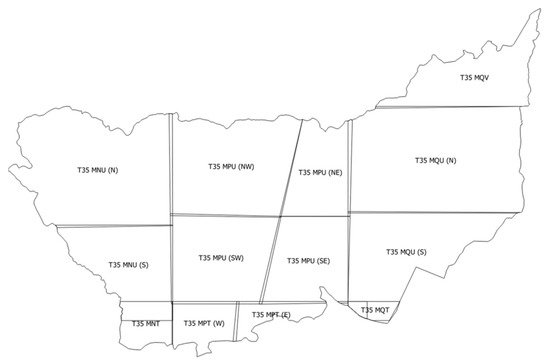
Figure 3.
Division into subtiles of the AOI.
2.3.2. Open Datasets
Very High Resolution Satellite Imagery (VHRSI) was used for photo interpretation and validation/refinement of classification results, especially in those areas with clouds or shadows in any tile [60]. VHRSI provides real colour ortho-photos with a spatial resolution between 0.5 and 2 m, which are widely used in RS [61,62]. Specifically, web-accessible BING Aerial ortho-photos (updated 2018) were used [63]. Open Street Map (OSM) data were also used to map roads, water bodies and residential areas. We obtained OSM data in vector format from the online platform [64]. For the present research, we appropriately rasterised data at the 10 m grid size.
2.3.3. Reference Datasets
A ground survey campaign was performed throughout the entire diocese area to test the accuracy of LULC classification. One hundred GRPs were acquired using a Garmin GPSMAP 64 GNSS (Global Navigation Satellite System) receiver with a nominal positional accuracy of 5 m (Figure 4). For each GRP three data were acquired: planimetric position (according to the WGS84 UTM 35S GPS-acquiring Reference System–RS), a high-definition camera picture portraying the local LULC with annotated exposure, and the classification of local land use near that position into four main classes (i.e., Forest, Agriculture, Pasture and Non-vegetated areas). We then generated a reference polygon layer containing Control Polygons (CPs) to assess the classification of the agricultural production system in the Katoyi Collectivity. In particular, 200 CPs were selected randomly in Katoyi, based on the CP layer. One hundred CPs were selected from the “Agriculture” class as defined by the LULC classification; the remaining 100 CPs were selected from the “Pasture” class. Using VHRSI, a photo-interpretation of the CPs was performed via searching for SOA and BOA within the LULC classes. Figure 5 shows the CPs’ distribution in the study area.
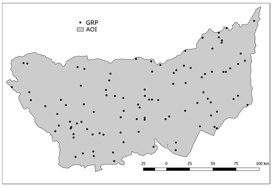
Figure 4.
GRP distribution in the study area.
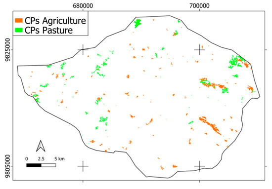
Figure 5.
The CPs’ distribution in Katoyi collectivity (Reference Frame: WGS84/UTM35S).
2.4. Object-Based Classification in the Goma Diocese
An object-based classification (OBC) approach [65,66] was used for this work. This approach was based on the supervised classification carried out in four main steps: (a) S2 data segmentation; (b) training feature selection based on segmented objects; (c) object classification adopting a minimum distance algorithm; (d) cloud masking correction.
2.4.1. Segmentation
OBC divides a multi-spectral image into groups of spectrally homogeneous pixels while respecting some geometric constraints. Pixels from the processed image are consequently aggregated according to constraints (parameters) that the operator has to properly set up by considering the expected minimum object size and its maximum internal spectral heterogeneity. The segmentation step of the OBC approach was performed using the mean-shift algorithm available in Orfeo Toolbox v.6.6.0 open software [67,68]. The OBC algorithm aimed at minimising the spectral heterogeneity of polygons by comparing the spectral properties of neighbour pixels. The resulting segmentation vector layer (SEG) was generated according to an a priori defined minimum mapping unit of 5000 m2.
Segmentation was carried out with particular reference to the S2 bands having the finest GSD = 10 m, i.e., B2, B3, B4 and B8. Starting from the native BOA reflectance values, images were divided into segments with an internally homogeneous spectral response. Segments were then vectorised to generate the corresponding vector layer. During segmentation, required parameters were set to the values reported in Table 3.
Table 3.
Parameters used during image segmentation.
SEG was then used to explore internal features other than spectral signatures, such as recurrent radiometric patterns (texture) and shape. These were adopted in the second level of analysis to better interpret SEG meaning, and, for this work specifically, to investigate land fragmentation schemes possibly related to different agricultural management types.
2.4.2. ROIs Selection
A false-colour image (FCI) was generated starting from mosaicked S2 bands, including B8, B4 and B3 in the channels of Red, Green and Blue respectively. Thirteen FCI classes were defined by searching for a specific land cover class, according to Appendix A, Table A1. Subsequently, 5491 regions of interest (ROIs) were randomly selected and photo-interpreted according to FCI classes. Figure 6 shows the ROIs’ locations. The total area of the ROIs corresponded to 1.6% of the entire surface of the GD. Table 4 reports the land cover classes adopted and the relative codes.
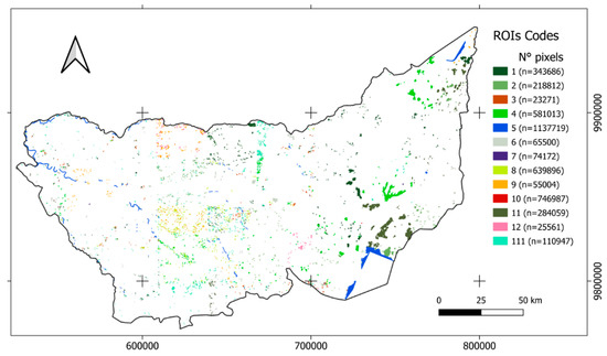
Figure 6.
Locations and number of pixels of ROIs (Reference Frame: WGS84/UTM35S).
Table 4.
Land cover codes.
Figure 7 shows the average spectral signature of each ROI class according to the codes in Table 4. Since available S2 cloud masks could be ineffective in complete cloud detection, especially cirrus clouds [69], and considering the coarse geometric resolution of this mask (GSD = 60 m), to better map these classes, clouds and shadows were considered in the classification by adopting bands with a GSD of 10 m. In fact, Coluzzi [69] found that S2 cloud masks over rainforest areas had an omission error of more than 70%.
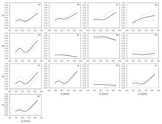
Figure 7.
ROIs’ spectral signatures. Bold line represents the mean value; dotted lines are mean value ± 1 standard deviation. (a) Dense Forest-1; (b) Sparse Forest-111; (c) Open Forest-2; (d) Bare Soil/Urban-3; (e) Grassland and lower vegetation-4; (f) Water-5; (g) Clouds-6; (h) Cloud Shadows-7; (i) Lower vegetation with strong vigour-8; (j) Agronomical field-9; (k) Wetlands and burned areas-10; (l) Fragmented croplands-11; (m) Croplands-12.
2.4.3. “Minimum Distance” Classification
A supervised OBC relies on a minimum distance algorithm approach. Different works have highlighted the performance and capability of such a classifier when applied to agricultural case studies [70,71,72].
Exploiting the B2, B3, B4 and B8 S2 bands, the relative mean value was computed at the patch level and added to the attribute table, starting from the SEG layer. Each patch’s spectral signature was classified based on ROI training features, adopting the minimum distance algorithm tool available on SAGA GIS v. 7.0.0. The land cover map was finally created, adopting the previously mentioned class codification.
2.4.4. Cloud Masking Correction
As the land cover classification was still affected by cloud cover contamination, the patches classified as clouds and cloud shadows were selected and substituted with the real land cover class retrieved from VHRSI photo-interpretation.
2.4.5. Land Use Class Aggregation
Thirteen land cover classes characterised the map obtained by the classification. These classes were initially chosen to better cope with the spectral variability among all the land cover types featured in the study area, but to restrict the focus on vegetation-related LULC classes, fewer classes were sufficient. Therefore, classes were merged as indicated in Table 5 to finally obtain a five land-use classification consisting of forests (coded as 1), agricultural (coded as 2), pasture (coded as 3), non-vegetated (coded as 4), and water (coded as 5). The class “water” was excluded in the successive validation step, as it was not relevant to the aim of this work.
Table 5.
Land cover and LULC codes adopted.
The accuracy of the LULC map was tested against the GRPs by comparing classes defined by ground-based methods with those classified by the minimum distance algorithm. A confusion matrix was then produced to evaluate both classification performances.
2.5. Classification of the Production Systems in Katoyi
In this work, NDVI entropy (HNDVI) was assumed as an appropriate image texture parameter able to separate the agricultural production systems of interest. In fact, building on the description of the two existing production systems, we assumed that in BOA production systems the vegetated areas (patches) would show a more homogeneous NDVI distribution, corresponding to lower HNDVI values. Conversely, in SOA production systems vegetated areas would be more heterogeneous and fragmented, making HNDVI of these patches higher. With these premises, the most critical aspect in the workflow was the identification of an appropriate HNDVI threshold able to separate the two production systems (i.e., SOA and BOA). Obviously, an objective and generally viable threshold does not exist. Consequently, an adaptive method was implemented, which was based on an iterative process, looking for the HNDVI value that minimises classification commission and omission errors while maximising the corresponding overall accuracy and class separability.
To this aim, an NDVI map [73] was calculated to describe vegetation biomass starting from multispectral mosaics, shown in Equation (1):
where NIR and RED are S2 B8 and B4 reflectance values, respectively.
HNDVI index was then calculated according to Equation (2) to assess local vegetation heterogeneity [41]:
where NDVIi,j is the NDVI value at the ith row and jth column in the local square window with a size of N pixels. For this study, the authors adopted a window size of 10 × 10 pixels. Finally, an HNDVI map was generated. The average HNDVI value was calculated at the patch level of the SEG layer. Only patches belonging to agriculture and pasture classes were considered in order to better characterise these LULC types. To do this we adopted the following interpretative key: Low HNDVI values meant homogeneous vegetated surfaces; high HNDVI meant highly heterogeneous vegetation, probably mixed with bare soil, or coexistence of vegetation covers with variable height and density [74].
Two binary classifications based on an entropy value threshold were performed for agriculture and pasture classes, respectively. The confusion matrix parameters were calculated according to Richards et al. [75] and using the CPs as references. In particular, class separability was estimated using the Jeffries–Matusita index (JM) according to Equation (3):
in which
where Ci and Cj are the within-class covariance of the ith and jth classes respectively, and mi and mj are the means of the ith and jth classes respectively. A JM distance equal to 2.0 implies 100% separability between two classes [76]. Therefore, 10 classifications were generated for agriculture LULC based on the following HNDVI threshold values: 0.3; 0.4; 0.5; 0.6; 0.7; 0.8; 0.9; 1.0; 1.1; 1.2; while eight classifications were generated for pasture LULC based on thresholds of 0.3; 0.4; 0.5; 0.6; 0.7; 0.8; 0.9; 1.0. The binary classification minimising commission and omission errors and maximising overall accuracy and JM was assumed to be the most reliable for classifying agriculture and pasture production systems.
3. Results and Discussion
3.1. LULC of the Goma Diocese
The entirety of the GD was divided into four classes of LULC: forest, agricultural, pasture and non-vegetated areas (Figure 8). Roads and water bodies were obtained from OSM data and overlapped on the LULC map, since they were not relevant for the work focused on vegetation-related classes.
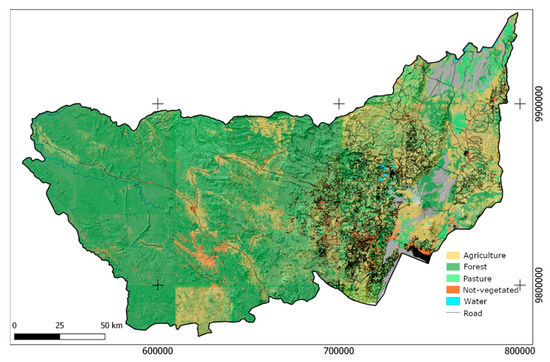
Figure 8.
LULC map based on OBC (Reference Frame: WGS84/UTM35S).
As shown in Table 6, the most widespread class was forest, with an extent of 15,629.13 km2 corresponding to 59% of the GD. The agricultural class covered 5106.25 km2 and the pasture class 3593.71 km2, corresponding to shares of 19% and 13%, respectively. By observing the maps, it is possible to note that the areas containing forests were mainly located in the central-western part of the GD, while agricultural and pasture land were more represented in the central-eastern zone.
Table 6.
Extent of LULC classes in GD.
Table 7 shows the confusion matrix related to the LULC classification produced in the GD. The classification performance resulted in an overall accuracy (OA) of 0.55; producer accuracy (PA) and user accuracy (UA) values (Table 7) are helpful to better clarify the strengths and weaknesses of this result.
Table 7.
Confusion matrix of LULC. UA = User Class Accuracy, PA = Producer Class Accuracy, CE = Commission Error, OE = Omission Error.
In particular, the classification was accurate in recognising “forest and urban” and “bare soil” classes, since their spectral signatures were clearly separable from the others. On the other hand, there was an overlap between agricultural and pasture classes, since these have a similar spectral signature, which makes their separation difficult.
A multi-temporal approach can investigate vegetation’s phenological behaviour, improving the separation between these classes [77]. Unfortunately, the adopted approach (based on single mosaicked acquisition) was dictated by the intense cloudiness that generally characterises equatorial areas, making it impossible to collect a series of contiguous images in space-time.
3.2. Production System Identification in Katoyi Collectivity
The binary classifications for agriculture and pasture production systems were defined according to the confusion matrix and JM parameters (Figure 9), searching for the HNDVI threshold value that minimised Omission Error (OE) and Commission Error (CE) for both classes and at the same time maximised the OA and the JM values. The HNDVI value of 0.7 was identified as the best for both the LULC classes (Figure 9).
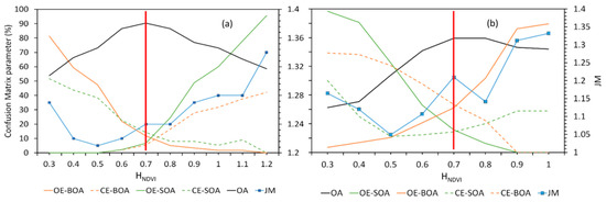
Figure 9.
Accuracy parameters used to select the NDVI entropy threshold (HNDVI, red vertical line) to generate a binary classification of rural production systems. (a) Agriculture LULC accuracy. (b) Pasture LULC accuracy. Omission and Commission Errors (OE and CE) produced during Business Oriented Agriculture systems classification (OE-BOA and CE-BOA) are marked by solid and dotted orange lines, respectively. Omission and Commission Errors generated during Subsistence Oriented Agriculture systems classification (OE-SOA and CE-SOA) are marked by solid and dotted green lines. The overall accuracy (OA) is represented by solid black lines and the Jeffries–Matusita (JM) values are depicted by blue lines.
By adopting this threshold, the OA and JM of agriculture LULC were equal to 90% and 1.24, while OE and CE were lower than 15% for both BOA and SOA. Concerning pasture LULC, OA and JM were equal to 80% and 1.22 while OE and CE were lower than 30% for both BOA and lower than 20% for SOA. All other tested thresholds in the range 0.3 < HNDVI < 1.2 showed lower OA and higher OE/CE.
It is worth remembering that an interpretation of HNDVI behaviour is needed to determine the meaning of classes. This interpretation was achieved by looking for HNDVI class distributions (Figure 10). High entropy in the agriculture class denoted strong spectral variability within each patch, probably related to bare soil/vegetation alternation typical of SOA; inversely, in the BOA a low variability index of vegetation was expected due to homogeneous management of the surface. Conversely, for the pasture class the meaning of entropy changed; in fact, in a pasture system the rate use of vegetation follows grazing pressure [78,79]. High grazing pressure generates a homogeneous consumption of pasture, thus a low HNDVI value within each patch. SOA is characterised by small grazing surfaces and intensive local use of pastoral resources. Ordinarily, a BOA pasture system has large surfaces (low grazing pressure) [80], which results in heterogeneous consumption of pasture and increasing HNDVI values.
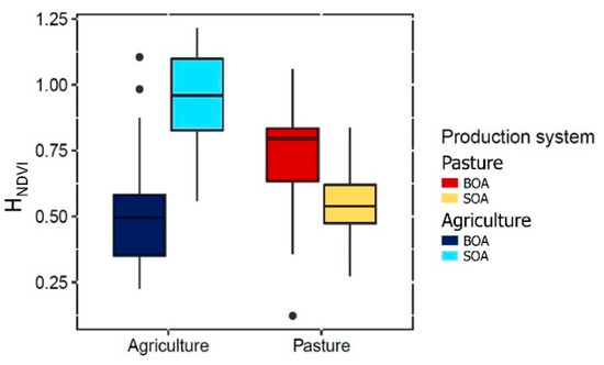
Figure 10.
HNDVI boxplots for Katoyi agriculture and pasture LULC classes. (Orange) BOA systems; (Green) SOA systems.
With this interpretative key, a final production systems map (Figure 11) was generated as follows: in the agriculture class, all patches with average HNDVI ≥ 0.7 were classified as SOA, while patches with HNDVI < 0.7 were classified as BOA. In the pasture class, the same principle was applied in inverse.
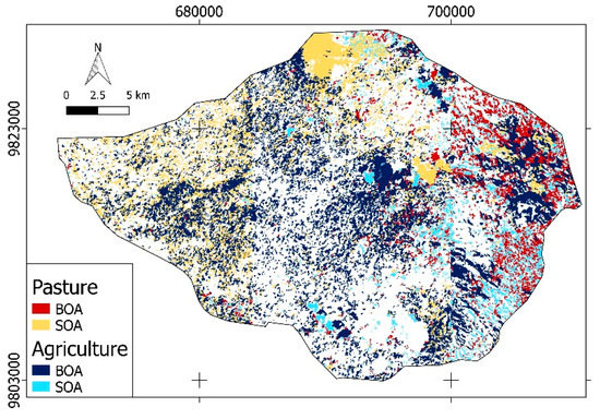
Figure 11.
Map representing agriculture and pasture production systems in Katoyi (Reference Frame: WGS84/UTM35S).
The total hectares ascribed to BOA and SOA in Katoyi collectivity are reported in Table 8. These results proved the prevalence of BOA production systems compared to SOA in Katoyi, and seem to confirm the portrait of a region where land scarcity for smallholders is becoming more and more relevant, especially where the dispute between large landowners and subsistence farmers is a perpetuating factor of conflict [2]. This result seems to agree with the unpublished results of a survey, conducted in 2017 by Caritas Development Goma, estimating that large landowners control approximately 80% of the land in the GD1. On the other hand, the validity of the methodology and the obtained accuracy in classifying the existing production systems could not be compared with those of other studies, due to the lack of research applying the same methodology in this region [81]. To the best of our knowledge, the only similar studies focus on different regions and address classification through different methodology, built on different available data, while obtaining comparable accuracy and methodological validity [82,83].
Table 8.
Agriculture and pasture production system areas in Katoyi according to the LU map produced.
The proposed methodology and the specific approach for determination of an appropriate entropy threshold value were applied to increase the procedure’s general applicability. In fact, both the adoption of publicly available data and the introduction of processing steps specifically aimed at reducing/avoiding subjective decisions were the basis for our work. This made it possible to calibrate HNDVI threshold value depending on the local distribution and value of NDVI at the patch scale, both of which strictly depend on local land management. Consequently, the HNDVI threshold values reported in this work cannot be assumed a priori but need to be determined empirically. However, the approach for their determination is general and adaptable and, therefore, usable anywhere around the world provided that ground reference data (here CPs) are collected to make the computation of classification errors possible.
4. Conclusions
In this work, S2 multispectral images were used to assess LULC in the GD. Specifically, a first land cover map was produced using an object-based supervised classification approach to detect and characterise land use in the GD. Comparable classification accuracy was found in a previous study [84], reinforcing S2’s data reliability when applied in the African context. Furthermore, in line with past research experience [66,85], the joint use of S2 and segmentation procedures proved to be effective in mapping and characterising agricultural and forest contexts. Nevertheless, some problems persisted. For instance, in SOA, where small heterogeneous areas were present and the algorithm could not systematically recognise fields, the delineation proved to be highly sensitive to segmentation parameters.
Starting from the identified LULC agriculture and pasture classes, a classification of agriculture production systems was created based on HNDVI value at the patch level. Since we presumed only two existing production systems (i.e., BOA and SOA), we proposed a binary threshold classification method. Such an approach is undoubtedly affected by threshold selection, and many works have examined this problem [86,87]. In this work, we proposed a retrospective method to define the best threshold and generate a binary classification. This threshold was defined by an optimisation procedure based on confusion matrix parameters and class separability. Specifically, we found that 0.7 HNDVI was the threshold that minimised CE and OE and maximised OA and class separability (the JM index) simultaneously for both agriculture and pasture. Some critical points still persist here: (a) more reference data (in this work, partially produced by photo interpretation) are needed to calculate confusion matrix parameters; (b) imbalanced data in the binary classification could affect results [88,89]; (c) further interpretation is needed to correct class meaning in order to avoid the introduction of bias. Nevertheless, we found that correcting class meaning through the HNDVI distribution between classes was a useful tool for classifying agriculture production systems; OA was found to equal 90% and 80% for agriculture and pasture, respectively.
Overall, the obtained results led us to conclude that RS was a useful tool for spatial analysis of land distribution among different agricultural production systems, even in equatorial regions characterised by complex orography and wide agricultural landscapes. This is extremely interesting in a region such as North Kivu and particularly the GD, where digital cadastres do not exist and the orography and chronic security issues result in difficult access to land-related information. In the framework of the Congolese path towards pro-poor agrarian land tenure reform that should regulate the increasing trend towards land ownership concentration, and in the context of an increasing rural population that strives for access to land, this information is fundamental for supporting both evidence-based interventions at national policy level, and international development cooperation operating within the country.
Research Perspectives
In this study, we obtained interesting results on a pilot-area scale (Katoyi collectivity); therefore, it would be very interesting to scale up this approach to the whole GD area. Across the world, there are several examples of countries where pro-poor land tenure reforms are struggling to see light due to specific, often-inscrutable political, security and geographical contexts. Knowledge regarding the distribution of different production systems may be the key information to trigger or support pro-poor reforms. Several cases exist in Africa where the proposed methodology may be trialled and therefore further improved and validated. Specifically, it is worth highlighting that a more robust validation of the proposed method could be obtained by repeating the implementation in several other case studies and by using ground-reference data systematically. The repetition in such contexts would fall under a Science Diplomacy approach [90], which uses applied research to foster diplomacy and social innovation uptake concerning delicate issues such as rural reforms in the framework of the 2030 Agenda.
Among the main critical issues to be improved, the region-specific constraint regarding cloud coverage could be overcome by coupling multispectral passive remote sensing with active remote sensing SAR (Synthetic Aperture RADAR) data (e.g., Sentinel-1). In fact, SAR sensors can penetrate cloud cover, and the polarisation properties of the backscatter signal and its temporal behaviour could more extensively describe land use classes. SAR data would also facilitate the adoption of a multi-temporal approach to the analysis of LULC and production systems, possibly improving the classification accuracy.
Nowadays, new software and algorithms such as Google Earth Engine (GEE) can improve remotely sensed data processing and allow data computation for large areas.
Future developments may concern the joint use in GEE of SAR and optical data, and the exploitation of alternative classification approaches (e.g., Random forest or TensorFlow).
Finally, a pixel-based approach to the analysis of VHRSI could also be tested and compared to the proposed methodology to assess the margin of improvement in classification accuracy.
Author Contributions
Conceptualization, P.D.M., S.D.P., G.M., G.S. and E.M.B.; methodology, S.D.P. and E.M.B.; software, E.M.B.; validation, G.S. and E.M.B.; formal analysis, S.D.P., F.S., E.J.M., T.O. and G.C.; investigation, P.D.M. and G.M.; data curation, P.D.M., S.D.P., G.C. and G.M.; writing—original draft preparation, P.D.M., S.D.P., F.S., E.J.M. and T.O.; writing—review and editing, P.D.M., S.D.P., F.S. and G.M.; visualisation, P.D.M., S.D.P. and F.S.; supervision, G.S. and E.M.B. All authors have read and agreed to the published version of the manuscript.
Funding
This research was funded by the ARDST project within the EU strategy for peace seeking and keeping operations in the African Great Lakes region (Grant No. 360149 of ICSP–Instrument contributing stability and peace).
Data Availability Statement
The data presented in this study are available on request from the corresponding author. The data are not publicly available due to credit restrictions.
Acknowledgments
The framework for this study is provided by a three-year EU-funded project called ARDST “Appui au retour de réfugiés et déplacés par le biais de la sécurisation de terres en Diocèse de Goma”, led by Caritas Development Goma NGO. The project started in February 2016 and ended in June 2019. We would like to acknowledge the fundamental role of the whole ARDST project team, particularly Gabriel Habimana, Janvier Kashori, Henri Kambesa, Claude Sibomana Ntwari, Joseph Habyarimana Ntangi, Robert Akilimali, Joseph Mvuyekure, Théoneste Buzakare, Guido Semahane, Serge Kwisila, Milabyo Malekela, Bertin Kibanja Mishiki, Christophe Sibomana, Michel Iyanya and Patrick Nsengiyumva.
Conflicts of Interest
The authors declare no conflict of interest. The funders had no role in the design of the study; in the collection, analyses, or interpretation of data; in the writing of the manuscript, or in the decision to publish the results.
Appendix A. Coding Adopted for Photointerpretation of FCI
Table A1.
False-colour image (FCI) from mosaicked S2 bands, used to create thirteen land cover classes classes used in turns to define Regions of Interest.
Table A1.
False-colour image (FCI) from mosaicked S2 bands, used to create thirteen land cover classes classes used in turns to define Regions of Interest.
| Land Cover Classes | Codes | FCI Example |
|---|---|---|
| Dense Forest High Vigour | 1 |  |
| Dense Forest Low Vigour | 111 |  |
| Open Forest | 2 |  |
| Bare soil/urban | 3 |  |
| Sparse vegetation low vigour | 4 |  |
| Low vegetation—high vigour | 8 |  |
| Ploughed fields | 9 |  |
| Wet or burned areas | 10 |  |
| Fragmented agricultural areas | 11–12 |  |
Note
| 1 | Within the framework of the ARDST Project, we supervised the implementation of a survey targeting the holders of land concessions in the Goma Diocese, aiming to collect data regarding existing conflicts concerning access to land. The survey allowed for the collection of 2558 observations. Surveyed concessions covered 173,526.3 ha (equal to 1735.26 km2, on 8609.96 km2 of agricultural and pasture area in GD). Concessions greater than fifty hectares comprised a share of 84% of the surveyed area. |
References
- Naidoo, S. The War Economy in the Democratic Republic of Congo; Institute for Global Dialogue: Pretoria, South Africa, 2003; ISBN 1-919697-63-2. [Google Scholar]
- Pottek, E.; Kasisi, R.; Herrmann, T. Land Tenure and Conflict Propagation: Critical Geopolitics from the Rural Grassroots in North Kivu (Democratic Republic of Congo). Cah. Géographie Québec 2016, 60, 83–125. [Google Scholar] [CrossRef][Green Version]
- Betge, D. Land Governance in Post-Conflict Settings: Interrogating Decision-Making by International Actors. Land 2019, 8, 31. [Google Scholar] [CrossRef]
- Mathys, G.; Vlassenroot, K. “It’s Not All about the Land”: Land Disputes and Conflict in the Eastern Congo. Rift Val. Inst. PSRP Brief. Pap. 2016, 1–8. [Google Scholar]
- Hesselbein, G. The Rise and Decline of the Congolese State: An Analytical Narrative on State-Making; Department of International Development of the London School of Economics: London, UK, 2007. [Google Scholar]
- Mutambala, A. Development and Underdevelopment: An Examination of Land Grabbing in the DRC. Bachelor’s Thesis, Lund University, Lund, Sweden, 2017. [Google Scholar]
- CIRGL. Déclaration de Dar-Es-Salaam Sur La Paix, La Sécurité, La Démocratie et Le Développement Dans La Région Des Grands Lacs; Conférence Internationale sur la Paix, la Sécurité, la Démocratie et le Développement dans la Région des Grands Lacs: Dar es Salaam, Tanzania, 2006. [Google Scholar]
- Chen, Y.; Fei, X.; Groisman, P.; Sun, Z.; Zhang, J.; Qin, Z. Contrasting Policy Shifts Influence the Pattern of Vegetation Production and C Sequestration over Pasture Systems: A Regional-Scale Comparison in Temperate Eurasian Steppe. Agric. Syst. 2019, 176, 102679. [Google Scholar] [CrossRef]
- European Commission Joint Communication to the Council: A Strategic Framework for the Great Lakes Region. In Proceedings of the High Representative of the Union for Foreign Affairs and Security Policy; European Commission: Brussels, Belgium, 2013.
- UNDP. Building Peace and Advancing Development in the Great Lakes Region; UNDP Publishing: New York, NY, USA, 2013. [Google Scholar]
- FAO. Family Farming Knowledge Platform–Democratic Republic of Congo; FAO: Rome, Italy, 2020. [Google Scholar]
- Molinario, G.; Hansen, M.C.; Potapov, P.V.; Tyukavina, A.; Stehman, S.; Barker, B.; Humber, M. Quantification of Land Cover and Land Use within the Rural Complex of the Democratic Republic of Congo. Environ. Res. Lett. 2017, 12, 104001. [Google Scholar] [CrossRef]
- Molinario, G.; Hansen, M.; Potapov, P.; Tyukavina, A.; Stehman, S. Contextualizing Landscape-Scale Forest Cover Loss in the Democratic Republic of Congo (DRC) between 2000 and 2015. Land 2020, 9, 23. [Google Scholar] [CrossRef]
- Babu, S.C.; Gajanan, S.N.; Sanyal, P. Chapter 3—Effects of Commercialization of Agriculture (Shift from Traditional Crop to Cash Crop) on Food Consumption and Nutrition—Application of Chi-Square Statistic. Food Secur. Poverty Nutr. Policy Anal. 2014, 2, 63–91. [Google Scholar]
- Otchia, C.S. Agricultural Modernization, Structural Change and pro-Poor Growth: Policy Options for the Democratic Republic of Congo. J. Econ. Struct. 2014, 3, 8. [Google Scholar] [CrossRef]
- FAO. The State of Food and Agriculture–Leveraging Food Systems for Inclusive Rural Transformation; FAO Publishing and Multimedia Service: Rome, Italy, 2017; ISBN 978-92-5-109873-8. [Google Scholar]
- FAO. Analyse de La Résilience Au Nord Kivu, La République Démocratique Du Congo; Kowanko, N., Wiles, A., Baughan, E.C., Freeman, P., Blicke, F.F., Burckhalter, J.H., Plamondon, J., Alder, K., Eds.; Food and agriculture organization of the United Nations: Rome, Italy, 2019; Volume 13, ISBN 978-92-5-131205-6. [Google Scholar]
- Jacobs, C.; Mugenzi, J.R.; Kubiha, S.L.; Assumani, I. Towards Becoming a Property Owner in the City: From Being Displaced to Becoming a Citizen in Urban DR Congo. Land Use Policy 2019, 85, 350–356. [Google Scholar] [CrossRef]
- Marivoet, W.; Ulimwengu, J.M.; Vilaly, E.; Abd Salam, M. Understanding The Democratic Republic of the Congo’s Agricultural Paradox: Based on the EAtlas Data Platform; International Food Policy Research Institute: New York, NY, USA; Washington, DC, USA, 2018. [Google Scholar]
- Dominguez, L.; Luoma, C. Decolonising Conservation Policy: How Colonial Land and Conservation Ideologies Persist and Perpetuate Indigenous Injustices at the Expense of the Environment. Land 2020, 9, 65. [Google Scholar] [CrossRef]
- Koné, L.; Ngulungu, A.; Mbanzidi, N.; Kipalu, P.; Gata, T. Réforme Foncière et Protection Des Droits Des Communautés; FPP; RRN and DGPA: Kinshasa, Congo, 2016. [Google Scholar]
- Ministre des Affaires Foncières de la RDC. Reforme Fonciere: Document De Programmation Budgetaire; Mugangu, S., Mafine, B., Huart, A., Eds.; Primature: Kinshasa, Congo, 2017.
- CONAREF. Options Fondamentalales de Politique Fonciere Nationale; Forum Interprovincial Pour La Production Du Draft De La Politique Fonciere Nationale De La Republique Democratique Du Congo: Bukavu, Congo, 2018.
- CONAREF. Document de Politique–Draft 1; Commission Nationale de la Réforme Foncière; Minisère des affaires foncières de la RDC: Kinshasa, Congo, 2018.
- Rakundo, T.; Betge, D. The Land Reforms in the Democratic Republic of Congo–Practical Solutions for the Protection of Smallholder Land Rights; Annual World Bank Conference: Washington, DC, USA, 2020. [Google Scholar]
- Pech, L.; Lakes, T. The Impact of Armed Conflict and Forced Migration on Urban Expansion in Goma: Introduction to a Simple Method of Satellite-Imagery Analysis as a Complement to Field Research. Appl. Geogr. 2017, 88, 161–173. [Google Scholar] [CrossRef]
- Smets, B.; Michellier, C.; Syavulisembo, A.M.; Munganea, G.; d’Oreye, N.; Kervyn, F. Very High-Resolution Imaging of the City of Goma (North Kivu, DR Congo) Using SFM-MVS Photogrammetry. In Proceedings of the IGARSS 2018 IEEE International Geoscience and Remote Sensing Symposium, Valencia, Spain, 22–27 July 2018; pp. 3370–3373. [Google Scholar]
- Eisenberg, J.; Muvundja, F.A. Quantification of Erosion in Selected Catchment Areas of the Ruzizi River (DRC) Using the (R)USLE Model. Land 2020, 9, 125. [Google Scholar] [CrossRef]
- ESA. Land Cover CCI Product User Guide Version 2; UCL-Geomatics: London, UK, 2017. [Google Scholar]
- FAO. AFRICOVER: Land Cover Classification; FAO: Rome, Italy, 1997. [Google Scholar]
- Zelaya, K.; van Vliet, J.; Verburg, P.H. Characterization and Analysis of Farm System Changes in the Mar Chiquita Basin, Argentina. Appl. Geogr. 2016, 68, 95–103. [Google Scholar] [CrossRef]
- European Commission. INSPIRE Knowledge Base; European Commission: Bruxells, Belgium, 2020. [Google Scholar]
- Thyagharajan, K.K.; Vignesh, T. Soft Computing Techniques for Land Use and Land Cover Monitoring with Multispectral Remote Sensing Images: A Review. Arch. Comput. Methods Eng. 2019, 26, 275–301. [Google Scholar] [CrossRef]
- European Commission. Manual of Concepts on Land Cover and Land Use Information Systems; Office for Official Pubblication of European Communities: Luxembourg, 2000. [Google Scholar]
- Abdullahi, S.; Pradhan, B. Sustainable Brownfields Land Use Change Modeling Using GIS-Based Weights-of-Evidence Approach. Appl. Spat. Anal. 2016, 9, 21–38. [Google Scholar] [CrossRef]
- He, S.; Chung, C.K.L.; Bayrak, M.M.; Wang, W. Administrative Boundary Changes and Regional Inequality in Provincial China. Appl. Spat. Anal. Policy 2018, 11, 103–120. [Google Scholar] [CrossRef]
- Leisz, S.; Ha, N.; Yen, N.; Lam, N.; Vien, T. Developing a Methodology for Identifying, Mapping and Potentially Monitoring the Distribution of General Farming System Types in Vietnam’s Northern Mountain Region. Agric. Syst. 2005, 85, 340–363. [Google Scholar] [CrossRef]
- Mhangara, P.; Odindi, J. Potential of Texture-Based Classification in Urban Landscapes Using Multispectral Aerial Photos. S. Afr. J. Sci. 2013, 109, 1–8. [Google Scholar] [CrossRef]
- Mutoko, M.C.; Hein, L.; Bartholomeus, H. Integrated Analysis of Land Use Changes and Their Impacts on Agrarian Livelihoods in the Western Highlands of Kenya. Agric. Syst. 2014, 128, 1–12. [Google Scholar] [CrossRef]
- Senior, M.L.; Williams, H.C.W.L. The Varying Zone Size Effect and Dual Variables for Entropy Maximising Models of Spatial Interaction. Appl. Spat. Anal. Policy 2018, 11, 657–667. [Google Scholar] [CrossRef]
- Haralick, R.M.; Shanmugam, K.; Dinstein, I.H. Textural Features for Image Classification. IEEE Trans. Syst. Man Cybern. 1973, SMC-3, 610–621. [Google Scholar] [CrossRef]
- Chaluvadi, M.; Raghunadh, M.V.; Pullarao, C.; Kishore, M.S. Significance of Textural Features in Aerial Images. IETE J. Educ. 2012, 53, 9–20. [Google Scholar] [CrossRef]
- Li, M.; Zang, S.; Zhang, B.; Li, S.; Wu, C. A Review of Remote Sensing Image Classification Techniques: The Role of Spatio-Contextual Information. Eur. J. Remote Sens. 2014, 47, 389–411. [Google Scholar] [CrossRef]
- Ota, T.; Mizoue, N.; Yoshida, S. Influence of Using Texture Information in Remote Sensed Data on the Accuracy of Forest Type Classification at Different Levels of Spatial Resolution. J. For. Res. 2011, 16, 432–437. [Google Scholar] [CrossRef]
- Todd, M.C.; Washington, R. Climate Variability in Central Equatorial Africa: Influence from the Atlantic Sector. Geophys. Res. Lett. 2004, 31. [Google Scholar] [CrossRef]
- Wylie, D.; Eloranta, E.; Spinhirne, J.D.; Palm, S.P. A Comparison of Cloud Cover Statistics from the GLAS Lidar with HIRS. J. Clim. 2007, 20, 4968–4981. [Google Scholar] [CrossRef]
- Bendix, J.; Lauer, W. Die Niederschlagsjahreszeiten in Ecuador Und Ihre Klimadynamische Interpretation (Rainy Seasons in Ecuador and Their Climate-Dynamic Interpretation). Erdkdunde 1992, 118–134. [Google Scholar]
- Adejuwon, J.O. Rainfall Seasonality in the Niger Delta Belt, Nigeria. J. Geogr. Reg. Plan. 2012, 5, 51–60. [Google Scholar]
- Munzimi, Y.A.; Hansen, M.C.; Adusei, B.; Senay, G.B. Characterizing Congo Basin Rainfall and Climate Using Tropical Rainfall Measuring Mission (TRMM) Satellite Data and Limited Rain Gauge Ground Observations. J. Appl. Meteorol. Climatol. 2015, 54, 541–555. [Google Scholar] [CrossRef]
- Eberhardt, I.D.R.; Schultz, B.; Rizzi, R.; Sanches, I.D.; Formaggio, A.R.; Atzberger, C.; Mello, M.P.; Immitzer, M.; Trabaquini, K.; Foschiera, W. Cloud Cover Assessment for Operational Crop Monitoring Systems in Tropical Areas. Remote Sens. 2016, 8, 219. [Google Scholar] [CrossRef]
- UNDP. Poverty and Household Living Conditions in the North-Kivu Province; UNDP: New York, NY, USA, 2019. [Google Scholar]
- World Poverty Clock. World Poverty Clock; World Poverty Clock: Vienna, Austria, 2019. [Google Scholar]
- FAO. Farming Systems and Poverty 2001: Improving Farmers’ Livelihoods in a Changing World; Dixon, J., Gulliver, A., Gibbon, D., Eds.; FAO and the World Bank: Rome, Italy; Washington, DC, USA, 2001; Volume 39, ISBN 92-5-104627-1. [Google Scholar]
- De Marinis, P.; Sali, G. Participatory Analytic Hierarchy Process for Resource Allocation in Agricultural Development Projects. Eval. Program Plan. 2020, 80, 101793. [Google Scholar] [CrossRef]
- Tegera, A. La Conference de Goma et La Question de La Presence Des FDLR Au Nord et Sud Kiu: Etat Des Lieux; Pole Institute: Goma, Congo, 2008. [Google Scholar]
- ESA. Sentinel-2 User Handbook; ESA: Paris, France, 2015. [Google Scholar]
- ESA. ESA SciHub; ESA: Paris, France, 2020. [Google Scholar]
- Conrad, O.; Bechtel, B.; Bock, M.; Dietrich, H.; Fischer, E.; Gerlitz, L.; Wehberg, J.; Wichmann, V.; Böhner, J. System for Automated Geoscientific Analyses (SAGA) v. 2.1. 4. Geosci. Model Dev. Discuss. 2015, 8, 1991–2007. [Google Scholar] [CrossRef]
- Justice, C.O.; Townshend, J.R.G.; Holben, B.N.; Tucker, C.J. Analysis of the Phenology of Global Vegetation Using Meteorological Satellite Data. Int. J. Remote Sens. 1985, 6, 1271–1318. [Google Scholar] [CrossRef]
- Kassawmar, T.; Eckert, S.; Hurni, K.; Zeleke, G.; Hurni, H. Reducing Landscape Heterogeneity for Improved Land Use and Land Cover (LULC) Classification across the Large and Complex Ethiopian Highlands. Geocarto Int. 2018, 33, 53–69. [Google Scholar] [CrossRef]
- Agugiaro, G.; Poli, D.; Remondino, F. Testfield Trento: Geometric evaluation of very high resolution satellite imagery. Int. Arch. Photogramm. Remote Sens. Spat. Inf. Sci. 2012, XXXIX-B1, 191–196. [Google Scholar] [CrossRef]
- Brovelli, M.A.; Crespi, M.; Fratarcangeli, F.; Giannone, F.; Realini, E. Accuracy Assessment of High Resolution Satellite Imagery Orientation by Leave-One-out Method. ISPRS J. Photogramm. Remote Sens. 2008, 63, 427–440. [Google Scholar] [CrossRef]
- BING. BING Aerial Maps. 2020. Available online: https://cn.bing.com/maps (accessed on 8 December 2021).
- OSM. Open Street Map. 2020. Available online: https://www.openstreetmap.org/#map=4/38.01/-95.84 (accessed on 8 December 2021).
- Walter, V. Object-Based Classification of Remote Sensing Data for Change Detection. ISPRS J. Photogramm. Remote Sens. 2004, 58, 225–238. [Google Scholar] [CrossRef]
- Liu, D.; Xia, F. Assessing Object-Based Classification: Advantages and Limitations. Remote Sens. Lett. 2010, 1, 187–194. [Google Scholar] [CrossRef]
- Inglada, J.; Christophe, E. The Orfeo Toolbox Remote Sensing Image Processing Software. In Proceedings of the 2009 IEEE International Geoscience and Remote Sensing Symposium, Cape Town, South Africa, 12–17 July 2009; Volume 4, p. IV–733. [Google Scholar]
- Grizonnet, M.; Michel, J.; Poughon, V.; Inglada, J.; Savinaud, M.; Cresson, R. Orfeo ToolBox: Open Source Processing of Remote Sensing Images. Open Geospat. Data Softw. Stand. 2017, 2, 15. [Google Scholar] [CrossRef]
- Coluzzi, R.; Imbrenda, V.; Lanfredi, M.; Simoniello, T. A First Assessment of the Sentinel-2 Level 1-C Cloud Mask Product to Support Informed Surface Analyses. Remote Sens. Environ. 2018, 217, 426–443. [Google Scholar] [CrossRef]
- Wacker, A.G.; Landgrebe, D.A. Minimum Distance Classification in Remote Sensing; LARS Technical Reports; Purdue University: Lafayette, IN, USA, 1972. [Google Scholar]
- South, S.; Qi, J.; Lusch, D.P. Optimal Classification Methods for Mapping Agricultural Tillage Practices. Remote Sens. Environ. 2004, 91, 90–97. [Google Scholar] [CrossRef]
- Jog, S.; Dixit, M. Supervised Classification of Satellite Images. In Proceedings of the 2016 Conference on Advances in Signal Processing (CASP), Pune, India, 9–11 June 2016; pp. 93–98. [Google Scholar]
- Rouse, J.W., Jr.; Haas, R.H.; Schell, J.A.; Deering, D.W. NASA/GSFC, Type III, Final Report; NTRS-NASA Technical Reports Server: Greenbelt, MD, USA, 1974; p. 371.
- Fung, T.; Siu, W.-L. A Study of Green Space and Its Changes in Hong Kong Using NDVI. Geogr. Environ. Model. 2001, 5, 111–122. [Google Scholar] [CrossRef]
- Richards, J.A.; Jia, X. Remote Sensing Digital Image Analysis: An Introduction, 4th ed.; Springer: Berlin/Heidelberg, Germany, 2006; ISBN 978-3-540-25128-6. [Google Scholar]
- Richards, J.A.; Richards, J.A. Remote Sensing Digital Image Analysis; Springer: Berlin/Heidelberg, Germany, 1999; Volume 3. [Google Scholar]
- Sarvia, F.; De Petris, S.; Borgogno-Mondino, E. Multi-Scale Remote Sensing to Support Insurance Policies in Agriculture: From Mid-Term to Instantaneous Deductions. GIScience Remote Sens. 2020, 57, 770–784. [Google Scholar] [CrossRef]
- Adler, P.; Raff, D.; Lauenroth, W. The Effect of Grazing on the Spatial Heterogeneity of Vegetation. Oecologia 2001, 128, 465–479. [Google Scholar] [CrossRef]
- Lin, Y.; Hong, M.; Han, G.; Zhao, M.; Bai, Y.; Chang, S.X. Grazing Intensity Affected Spatial Patterns of Vegetation and Soil Fertility in a Desert Steppe. Agric. Ecosyst. Environ. 2010, 138, 282–292. [Google Scholar] [CrossRef]
- Mentis, M.T. Monitoring in South African Grasslands; Foundation for Research Development, CSIR: Delhi, India, 1984. [Google Scholar]
- Bégué, A.; Arvor, D.; Lelong, C.; Vintrou, E.; Simoes, M. Agricultural Systems Studies Using Remote Sensing. In Remote Sensing Handbook, Volume 2: Land Resources Monitoring, Modeling, and Mapping with Remote Sensing; CRC Press: Boca Raton, FL, USA, 2015; p. ffhal-02098284f. [Google Scholar]
- Crnojevic, V.; Lugonja, P.; Brkljac, B.; Brunet, B. Classification of Small Agricultural Fields Using Combined Landsat-8 and RapidEye Imagery: Case Study of Northern Serbia. J. Appl. Remote Sens. 2014, 8, 083512. [Google Scholar] [CrossRef]
- Vintrou, E.; Soumaré, M.; Bernard, S.; Bégué, A.; Baron, C.; Lo Seen, D. Mapping Fragmented Agricultural Systems in the Sudano-Sahelian Environments of Africa Using Random Forest and Ensemble Metrics of Coarse Resolution MODIS Imagery. Photogramm. Eng. Remote Sens. 2012, 78, 839–848. [Google Scholar] [CrossRef]
- Xiong, J.; Thenkabail, P.S.; Tilton, J.C.; Gumma, M.K.; Teluguntla, P.; Oliphant, A.; Congalton, R.G.; Yadav, K.; Gorelick, N. Nominal 30-m Cropland Extent Map of Continental Africa by Integrating Pixel-Based and Object-Based Algorithms Using Sentinel-2 and Landsat-8 Data on Google Earth Engine. Remote Sens. 2017, 9, 1065. [Google Scholar] [CrossRef]
- Immitzer, M.; Vuolo, F.; Atzberger, C. First Experience with Sentinel-2 Data for Crop and Tree Species Classifications in Central Europe. Remote Sens. 2016, 8, 166. [Google Scholar] [CrossRef]
- Nowakowski, A. Remote Sensing Data Binary Classification Using Boosting with Simple Classifiers. Acta Geophys. 2015, 63, 1447–1462. [Google Scholar] [CrossRef]
- Li, W.; Guo, Q. A New Accuracy Assessment Method for One-Class Remote Sensing Classification. IEEE Trans. Geosci. Remote Sens. 2013, 52, 4621–4632. [Google Scholar]
- Akosa, J. Predictive Accuracy: A Misleading Performance Measure for Highly Imbalanced Data. In Proceedings of the SAS Global Forum, Orlando, FL, USA, 2–5 April 2017; pp. 2–5. [Google Scholar]
- Guo, X.; Yin, Y.; Dong, C.; Yang, G.; Zhou, G. On the Class Imbalance Problem. In Proceedings of the 2008 Fourth International Conference on Natural Computation, Jinan, China, 18–20 October 2008; Volume 4, pp. 192–201. [Google Scholar]
- Ruffini, P.-B. Conceptualizing Science Diplomacy in the Practitioner-Driven Literature: A Critical Review. Humanit. Soc. Sci. Commun. 2020, 7, 124. [Google Scholar] [CrossRef]


Publisher’s Note: MDPI stays neutral with regard to jurisdictional claims in published maps and institutional affiliations. |
© 2021 by the authors. Licensee MDPI, Basel, Switzerland. This article is an open access article distributed under the terms and conditions of the Creative Commons Attribution (CC BY) license (https://creativecommons.org/licenses/by/4.0/).