Abstract
Landslides are the most common geodynamic phenomenon in Slovakia, and the most affected area is the northwestern part of the Kysuca River Basin, in the Western Carpathian flysch zone. In this paper, we evaluate the susceptibility of this region to landslides using logistic regression and random forest models. We selected 15 landslide conditioning factors as potential predictors of a dependent variable (landslide susceptibility). Classes of factors with too detailed divisions were reclassified into more general classes based on similarities of their characteristics. Association between the conditioning factors was measured by Cramer’s V and Spearman’s rank correlation coefficients. Models were trained on two types of datasets—balanced and stratified, and both their classification performance and probability calibration were evaluated using, among others, area under ROC curve (), accuracy (), and Brier score () using 5-fold cross-validation. The random forest model outperformed the logistic regression model in all considered measures and achieved very good results on validation datasets with average values of , , and . The logistic regression model results also indicate the importance of assessing the calibration of predicted probabilities in landslide susceptibility modelling.
1. Introduction
Landslides are one of the main natural hazards that put people’s lives at risk, cause damage to property, and require high costs in order to stabilise sites and protect investments in concerned areas when implementing investment projects. On the other hand, human activity significantly and frequently affects slope stability and unsuitably located building sites initiate slope movements. Landslide risk increases mainly through unregulated urbanisation, unsuitable land use, gradual deforestation, and removing continuous grassland vegetation cover. Landslides are influenced by changes in climatic conditions, mainly the character of regional precipitation, occurrence of torrential rains, and their distribution within yearly cycles.
Landslides belong to slope deformations that significantly affect the status and efficient use of land. They pose a constant threat mainly where there are construction sites without adequate measures. They repeatedly cause damage to land linear and other buildings, as well as to agricultural and forest soils. Nowadays, landslide risk in some regions of Slovakia is increasing as a result of more intensive construction activity shifting from flat and slightly inclined locations to slopes and more exposed locations. This trend is evident mainly in municipalities in mountainous areas of Slovakia. It is caused mainly by the lack of suitable construction sites in flat locations but also by targeted construction on slopes as a result of the attractiveness of the environment. For this reason, the need to assess the landslide susceptibility of the area, optimise forecasts of this phenomenon, and efficiently affect human activities in the area is constantly increasing.
The monitored area of Slovakia belongs to the Western Carpathian flysch area, where landslides are the most common geodynamic phenomenon. Landslide occurrence assessment in this area showed that fewer slope deformations occur in flysch highlands than in flysch uplands [1]. Geodynamic phenomena in flysch highlands are characterised mainly by extensive creep failure or landslides with mass movement on layered surfaces. Surface creep is typical mainly for flysch uplands and results in landslides and earth flows.
Maps of landslide susceptibility are useful tools for identifying future potential susceptible areas of landslide occurrence. They are used in land planning, forecasting natural risks, and mitigating measures [2]. The authors studied the influence of sensitivity and scaling issues in the landslide susceptibility mapping using random forests. They indicated that the unit (scale) and the training process strongly influence the classification accuracy and the prediction process. Maps of landslide susceptibility depict the relative probability of a given type of landslide occurring in a given area, without taking into consideration the probability of occurrence in time [3]. They explicitly or implicitly represent a forecast of future occurrences of the landslide areas [4]. They are based on comparing and subsequent statistical processing and assessing the spatial correlation between the predisposing factors (inclination, land use, geological bedrock, etc.), the landslide distribution in the area, and the time dimension of landslides connected to triggering events (precipitation, earthquake, volcanoes, and anthropogenic activities) [5,6]. These maps aim to provide a document that helps mitigate future damage to property and human health in the area. Mapping the landslide susceptibility of the area is crucial for safe planning of human activities, constructions, etc. [7]. At the regional level, landslide susceptibility maps represent the first efficient step in reaching detailed assessment and lowering landslide risk, which contributes to overall safety [8,9].
The landslide susceptibility assessment has improved significantly over the past years, in part because of implementing techniques based on statistics within GIS, see, e.g., in [10,11,12,13,14,15,16]. The landslide susceptibility assessment of the area can also be solved by deterministic methods, see, e.g., in [17,18,19,20], that take into consideration engineering characteristics of the rocks and soils, slope geometry, discontinuity characteristics, and hydrological conditions [7]. Another possible way to assess the landslide susceptibility can be by using statistical methods that determine which key factors are connected to the landslide. The authors use logistic regression, see, e.g., in [21,22,23,24,25,26]; discriminant analysis, see, e.g., in [27,28,29,30,31]; recently also artificial neural networks, see, e.g., in [31,32,33,34,35,36]; fuzzy logic, see, e.g., in [37,38,39]; neuro-fuzzy systems, see, e.g., in [40,41]; support vector machines, see, e.g., in [29,34,42,43,44]; and random forests, see, e.g., in [6,45,46,47,48]. Random forests is a nonlinear, nonparametric algorithm that can deal with large datasets containing both categorical and numerical data, and account for complex interactions and nonlinearity between variables. It can handle cases where there are more predictors than observations and incorporate interaction between multiple predictors, and is able to handle missing values and maintain accuracy for missing data [47]. It is used for large-scale mapping and classification applications in ecology, soil science, and flood mapping.
In the Czech Republic and Slovakia, many authors inquired into landslide susceptibility, see, e.g., in [49,50,51,52]. In their work, the authors of [49] evaluated 11 input parameters that were derived from geological conditions of the area, climatic and hydrological conditions, morphometry of the georelief, and the current landscape structure. The evaluation was processed by a bivariate method and the weight of the parameter as a whole. An important step in urban planning and proposals of land use for development is also producing and implementing models of landslide risk. The work in [53] is the only one to have used predictive modelling when evaluating landslide risk in Slovakia, who applied the Support Vector Machines method and compared it with the bivariate analysis. In all cases, it became apparent that the suitability of the used method is determined by the quality and the amount of the input data, required output data precision and their interpretability.
Landslides are often strongly correlated with multiple causes, resulting in complex parameterisations. Understanding the relationship between the existing soil landslide distribution and the soil landslide influencing factors is a fundamental requirement for soil landslide susceptibility mapping. This study aims to create a landslide susceptibility prognosis of the slopes in the study area using statistical predictive modelling for future use in land use planning. The fifteen generated layers of causative factors were used as predictor variables and were grouped into five classes: topographic, geological, hydrological, soil, and land cover. We chose two modelling methods: logistic regression and random forests. The resulting models were compared with the real occurrence of landslides. In this article, we comprehensively evaluate the susceptibility of flysch areas to landslides in the Western Carpathians, where this methodology has not yet been used. Until now, multivariate or bivariate analyses have been used here. The Kysuce region was selected as a model area as it belongs to the Western Carpathian flysch zone and is composed of sedimentary rocks, primarily sandstone, and clay. The characteristics of these rocks significantly affect the relief and water regime. They are prone to erosion and with their low permeability they can cause frequent landslides during torrential rains.
2. Study Area
The study area was defined as the entire river basin of the Kysuca River (Figure 1). It comprises the Čadca District (23 municipalities), Kysucké Nové Mesto District (14 municipalities), and a part of Žilina District (Lutiše Municipality). Based on the division of Slovakia into geomorphological units [54], the study area belongs to the sub-province Outer Western Carpathians. Its three areas—Stredné Beskydy Mts. (geomorphological units: Kysucké Beskydy, Oravské Beskydy, Kysucká vrchovina, Podbeskydská brázda, Podbeskydská vrchovina. Oravská Magura)—take up , Západné Beskydy Mts. (geomorphological units: Moravsko-sliezske Beskydy, Turzovská vrchovina, Jablunkovské medzihorie) and Slovensko-moravské Karpaty Mts. (geomorphological unit: Javorníky) take up . The height ranges from 325 m a.s.l. in Kysucká brána near Radol’a to 1236 m a.s.l at the top of Vel’ká Rača hill.
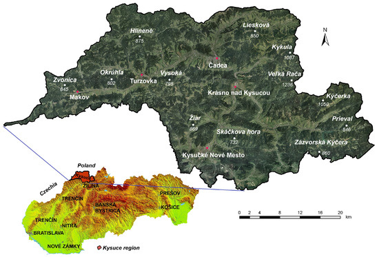
Figure 1.
The study area: Slovakia—Kysuce Region.
The Western Carpathian geological structure is mainly the result of alpine orogeny. The Outer Western Carpathians are formed by the Outer Subcarpathic flysch belt (Krosno and Magura units) and klippen belt (Orava unit—Mesozoic sediments) [55]. The flysch belt represents a massive accretionary wedge with a nappe structure. It is a Cretaceous Formation mainly from the Paleogene. It is a typical alternation of clay shales and sandstones that sedimented in a deep sea environment, where they were transported by gravitational and turbidity currents (Krosno and Magura units) [56].
Three fundamental tectonic units make up the geological structure of the area, from northwest to southeast it is Silesian Nappe, Magura Nappe, and Klippen Belt. The most common geological units in the area are the Zlín Formation ( ), deluvial sediments ( ), the Bystrica Unit ( ), and the Soláň Formation ( ). The Zlín Formation covers approximately one-third of the study area. This formation has higher susceptibility to landslides, which is caused mainly by the different geomorphological values of the claystone and sandstone sequence. The higher share of claystone results in greater susceptibility of this formation to exogenous degradation processes. They are mostly degraded due to frequent imbibition and drying processes resulting from higher precipitation rates.
From a precipitation perspective, Kysuce belongs to the humid climatic area. The average annual precipitation in the northern areas of the Kysuce valley is 700–1110 . The highest average monthly precipitation is in June and July (Table 1, data from the Slovak Hydrometeorological Institute). From a temperature point of view, Kysuce belongs to a cold and mildly warm climatic zone, with average yearly temperature in Čadca (2001–2020) (Table 2, data from the Slovak Hydrometeorological Institute). In the last decades, the average annual precipitation values and summer precipitation values have only a slightly decreasing trend. The area is mostly covered by coniferous forests ( ) that take up almost 52% of the area.

Table 1.
The average monthly total precipitation in Čadca for the period 1951–2020 (SHI).
Table 2.
The average monthly temperature in Čadca for the period 1951–2020 (SHI).
There are 1869 landslides registered in this area. Landslides are registered in the State Geological Institute of Dionýz Štúr databases and their locations were verified in the field. The database contains point landslides (those of small proportion) and area-wide landslides. The Atlas of slope stability maps SR [57] is the basis for digital layers that are continuously updated. Landslides take up almost 20% ( ) of the monitored area and the majority, 62%, occurred mainly due to climatic factors associated with erosion (lateral and deep) and abrasion. According to the activity, the landslides were divided into three categories: active, potential and stabilised (Figure 2). An active (live) landslide is a landslide in motion. If the motion is currently being suspended, but the causes of its formation can appear under suitable conditions, then the landslide is considered potential (temporarily suspended). In stabilised (permanently suspended—non-active) landslide the causes for its occurrence are no longer present, or they have been removed by human intervention. The majority of the landslides present in the study area, 70%, were classified as potential landslides, with a total of 1284 ( ). Stabilised landslides follow with 544 ( ), and then 41 active landslides ( ). For the purposes of the predictive modelling of landslide susceptibility the active and potential landslides were grouped together to form the landslide category and the stabilised landslides were assigned to the non-landslide category together with the landslide-free areas (see Figure 3p for the map of landslides as used during the modelling).
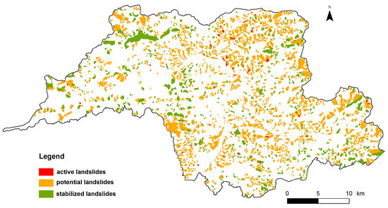
Figure 2.
Landslide activity in the study area.
3. Methods and Data
There is no global guideline for selecting landslide conditioning factors, but they should be selected based on the characteristics of the case study area, data availability, and literature review. One of the most important steps in spatial prediction modelling is selecting appropriate and effective conditioning factors among all available factors [58]. When selecting the input variables, we concentrated on those variables that can be triggers for landslides. They are geological, hydrogeological and soil properties, morphometric parameters of relief, hydrophysical soil properties, and hydraulic properties of rocks. We selected two methods of predictive modelling: logistic regression and random forests. In statistical modelling and subsequent evaluation, we proceeded as follows:
- selection of input variables and their reclassification,
- correlation analysis of the variables and their selection into statistical models,
- statistical modelling by logistic regression and random forests methods,
- interpretation of the individual methods, and
- evaluation of the landslide susceptibility of the area.
3.1. Variable Selection and Data Preparation
When selecting the input variables (landscape parameters), we used a database of landscape-ecological complex elements [59], which represents a vector representation of synthetic units expressing relevant characteristics of the abiotic component of the landscape sphere together with elements of land cover. When processing the data, we used real landslide occurrences registered in the State Geological Institute of Dionýz Štúr [57].
In connection to the environmental factors used in evaluation of landslide hazard, there is a tendency to use those layers of data that can be easily obtained from the digital model of relief and satellite images, while lesser emphasis was on those layers of data that needed detailed analysis in the field (environmental factors aimed at the digital model of the terrain, geology and soil, geomorphology, usage of the area and risk elements) [60,61,62]. Hydrological conditions, such as high precipitation and infiltration and exfiltration of groundwater, have strong influence on landslide occurrence [63]. Lithology of rocks and slope inclination are significant factors contributing to the higher activity of slides. When evaluating and mapping the susceptibility to landslides, the majority of authors use the degree of slope inclination and lithology as independent variables [21,64]. The authors of [65] divide factors influencing the occurrence of landslides into two types: external and internal factors. External factors comprise precipitation, earthquakes, and antropogenous factors. However, internal factors also deserve the attention—lithology of rocks, degree of slope inclination, location of the slope, profile of the slope, and elevation gradient.
We selected 15 conditioning factors that acted as input variables in the models of landslide susceptibility. Each of these 15 factors, except for altitude, was obtained in an individual vector layer. Altitude was obtained in a raster layer with grid cells. Therefore, to combine altitude with the other variables, the study area was divided into pixels (grid cells) of size and data properties of each pixel were attributed according to the majority representation of the individual variable classes in the given pixel. Furthermore, the selected modelling methods work better with pixels than with UCU-s and the advantages and disadvantages of both spatial units are comparable [66].
The selected variables are of different types which needs to be addressed during modelling. Of the 15 input variables all but one are categorical variables, with eight nominal (surface relief morphology, hydrogeological units, soil type, land cover, geological units, granulometry, profile curvature, and orientation) and six ordinal (inclination, transmissivity coefficient, filtration coefficient, groundwater level, soil depth, and soil skeleton). The last variable (altitude) is considered a continuous variable. The dependent variable (landslide susceptibility) was taken to be a binary variable.
Some of the classes of the categorical nominal variables contained a small number of pixels which may cause difficulties with interpreting the results during the modelling process and applying the models to other areas. Therefore, classes of the categorical nominal variables were reclassified into more general classes to address this. A list of all conditioning factors and their classes used in modelling and the landslide occurrence being modelled is provided below (visualisations of the occurrence of the variables in the study area can be found in Figure 3 and Figure 4):
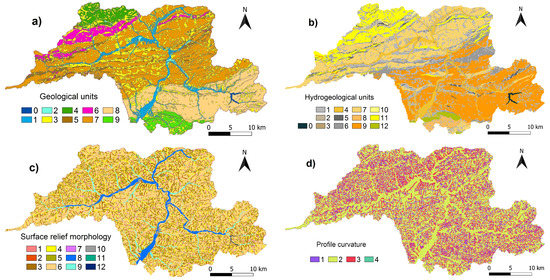
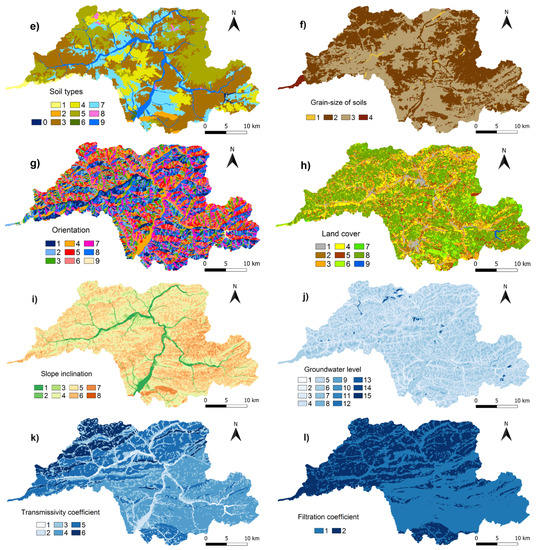
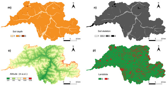
Figure 3.
Maps of conditioning factors and the map of landslides used in this study: (a) Geological units, (b) Hydrogeological units, (c) Surface relief morphology, (d) Profile curvature, (e) Soil types, (f) Grain-size of soils, (g) Orientation, (h) Land cover, (i) Slope inclination, (j) Groundwater level, (k) Transmissivity coefficient, (l) Filtration coefficient, (m) Soil depth, (n) Soil skeleton, (o) Altitude, (p) Landslide (figure legends—see Section 3.1).
- Geological units (GU) (Figure 3a)—a synthetic unit that complexly states the attributes of abiotic components of the landscape. Legend: 0 water; 1 fluvial sediments; 2 proluvial sediments; 3 deluvial sediments; 4 quartzy, arcosic and graywacky sandstones to conglomerates, dominance of black-brown shaly claystones, sandstones to pebbly sandstones and conglomerates; 5 medium grained sandstone to fine conglomerates, at places with biotite, local claystones, marlstones, intercalations of Bystrica-type claystones and quartzy sandstones (thin-layered flysch); 6 sandstone-shale facies: gray quartz and graywacky sandstones, green and grey shales, marlstones and pelosiderites (thin-layered flysch); 7 graywacky sandstones, local shales (sandy flysch); 8 Bystrica facies: Bystrica-type claystones, arcosic and graywacky sandstones with glauconite and conglomerates (flysch); 9 fine- to medium grained quartz carbonate sandstones, green-grey silty claystones, layered grey soft limestones with dark cherts, radiolarites, radiolarian limestones [67].
- Hydrogeological units (HGU) (Figure 3b)—units comprising lithology, lithostratigraphy of rocks, and hydrogeological properties of rock environment. Legend: 0 water; 1 lithofacial undivided loamy slope deposits, rocky soil and debris; 2 sandy-stony and boulder debris cones; 3 loams, sandy loams, sandy-loamy to boulderlike gravels in alluvial fans; 4 sands, sandy gravels and fine- to pebbly- gravels of terraces; 5 claystones, calcareous claystones and marlstone; 6 clayey flysch (flysch with claystones, siltstones and marlstones dominance); 7 normal flysch—claystones, siltstones and sandstones; 8 carbonate flysch (calcareous sandstones and marlstones); 9 sandy flysch (flysch with sandstone dominance); 10 conglomerate flysch (flysch with conglomerates dominance); 11 sandstones with claystones; 12 limestones, quartzy, sandy, marly and nodular limestones, radiolarites.
- Surface relief morphology (SRM) (Figure 3c)—represents a simple and homogenous geometric shape conditioned by homogenous form genesis. It is created based on digital terrain models (DTM) and derived from morphometric parameters with grid resolution 10 × 10 and we proceeded from basic topographical maps measuring scale 1:10,000. Legend: 1 flat top; 2 dome top; 3 ridge; 4 depression; 5 slope valley; 6 transport slope; 7 slope plateau; 8 wide riparian floodplain; 9 narrow floodplain of mountain stream; 10 outwash fan; 11 saddle; 12 the bottom of the dam.
- Profile curvature (PC) (Figure 3d)—represents the relief curvature in the direction of the contour (line). If the contour line is direct (linear), it means that all points lying on it have the same georelief orientation. The contour line curvature represents a change in georelief orientation in the direction of the contour line, thus a change in direction of the flow of matter and energy in georelief. Legend: 1 concave curvature; 2 linear curvature; 3 convex curvature; 4 complex curvature.
- Soil types (ST) (Figure 3e)—comprises a group of soils characterised by the same stratigraphy of the soil profile. Legend: 0 water; 1 Sceletic Leptosols; 2 Rendzic Leptosols, less frequent as Eutric Cambisols and Skeli-Rendzic Leptosols; 3 Eutric Cambisols, rarely Calcaric Cambisols; 4 Sceletic Cambisols, rarely Lithic Leptosols; 5 Dystric Cambisols; 6 Luvic Cambisols; 7 Stagnic Cambisols, rarely Stagnic Glossisols; 8 Umbril Podzols, less frequently Haplic Gleysols and very rarely Dystric Planosols; 9 Eutric Fluvisols and less frequently Haplic Histosols.
- Grain-size of soils (GSS) (Figure 3f)—division of soil based on the type of coarse grained clay. It is a hydrophysical property of soil, calculated using the SPAW model. Legend (categories are in % of clay fraction): 1 sandy-clay, rarely clay-sandy; 2 clay; 3 dusty-clay; 4 loamy-clay, less often sandy-loamy-clay and rarely dusty-loamy-clay.
- Orientation (Or) (Figure 3g)—orientation of the relief according to the cardinal points. It represents which cardinal point the inclined surface is oriented towards. It is morphometric characteristic that is derived in GIS based on DTM. Legend: 1 north ; 2 north-east ; 3 east ; 4 south-east ; 5 south ; 6 south-west ; 7 west ; 8 north-west ; 9 flat zone.
- Land cover (LC) (Figure 3h)—represents materialised projection of natural spatial determinateness (morpholocational and bioenergetical) and at the same time of the present landscape usage. Legend: 1 built up area, industrial, transport and business sites and sites of residential vegetation; 2 arable land; 3 mosaics of small-scale arable land and permanent grass vegetation; 4 meadows and grasslands with small representation of non-forest woody vegetation; 5 non-forest woody vegetation; 6 deciduous forests; 7 mixed forests; 8 coniferous forests; 9 bodies of water.
- Slope inclination (SIn) (Figure 3i)—expresses a continuous gradient field of the altitudes. It is a key morphometric parameter defining acute intensity of gravitationally conditioned geomorphological processes. It is a characteristic derived from a DTM, calculated in GIS using the algorithm “Neighbourhood method” [68]. Legend (categories are in degrees): 1 ; 2 ; 3 ; 4 ; 5 ; 6 ; 7 ; 8 .
- Groundwater level (GWL) (Figure 3j)—a continuous upper groundwater surface limit in the earth crust filling up its cavities. The data were acquired from hydrogeological drilling and engineer-geological probes. These measurements were then extrapolated using Spline interpolation algorithm that enabled the definition of the barriers. The layers of watercourse floodplains and areas according to the groundwater circulation type were defined as barriers (areas) for unique interpolation. Legend (categories are in meters): 1 ; 2 ; 3 ; 4 ; 5 ; 6 ; 7 ; 8 ; 9 ; 10 ; 11 ; 12 ; 13 ; 14 ; 15 .
- Transmissivity coefficient (TC) (Figure 3k)—a measure of aquifer ability of a certain thickness to permeate water with a given kinematic viscosity. Legend (categories are in ): 1 ; 2 ; 3 ; 4 ; 5 ; 6 .
- Filtration coefficient (FC) (Figure 3l)—a degree of a porous environment for water with a given kinematic viscosity. Legend (categories are in ): 1 permeable ; 2 medium to low permeable .
- Soil depth (SDe) (Figure 3m)—depth of soil profile from the soil surface to the eroded mother rock. Legend (categories are in meters): 1 shallow soils to , ; 2 medium-deep soils ; 3 deep soils and more.
- Soil skeleton (SSk) (Figure 3n)—proportion of soil particles bigger than 2 mm. Legend (categories are in % of the skeleton): 1 without skeleton or very little skeletal soils, only up to 10% of the skeleton, ; 2 small skeletal soils, 10 to 25% of the skeleton, ; 3 medium skeletal soils, 25 to 50% of the skeleton, ; 4 heavily skeletal soils, more than 50% of the skeleton, >50.
- Altitude (Alt) (Figure 3o)—continuous variable (from 325 m a.s.l. to 1236 m a.s.l.). It is a grid representation of the DTM with resolution 20 × 20 m that represents continuous variables of the height fields and respects the course of the current river network.
- Landslide (LS) (Figure 3p)—is the resulting morphological form of the slope movement caused by gravitation. Legend: 0—non-landslide area; 1—landslide area.
During landslide susceptibility modelling using the logistic regression the categorical nominal variables are transformed into binary indicator variables (where c is the number of classes for the given variable). The categorical ordinal variables were transformed to continuous variables by taking the middle of the interval the classes represent as their values, as was suggested in [69]. This still allows for the modelling of the nonlinear relationship between the landslide susceptibility and the input variables by adding the powers of the variables (e.g., slope).
After discarding pixels with missing values for some variables (these were the pixels corresponding to the Nová Bystrica reservoir), the dataset contained 4,223,653 pixels from which 550,896 were labelled as landslide areas.
3.2. Correlation Analysis of the Input Variables
A common feature of the real-world data is that the input variables (also called predictors) are not independent from each other. This may result in unstable estimates of the parameters which prevent identifying the variables relevant to modelling landslide susceptibility and interpreting their effects [70]. Therefore, the next step was to perform the correlation analysis for the input variables to determine the relation between them. The manner of measuring the association varies based on the type of variables (continuous, categorical ordinal, or categorical nominal).
To measure the association between the two categorical variables, we used Cramer’s V that is defined for two variables X and Y with categories and , respectively, where and , as
where n is the number of pixels; and are the number of pixels in categories and , respectively; and is the number of pixels that are in both and . Values of Cramer’s V lie between 0, indicating no association, and 1, indicating complete association. For calculating Cramer’s V the ordering of categories of categorical ordinal variables was neglected.
To measure the association between the continuous or categorical ordinal variables we used Spearman’s rank correlation coefficient that is defined as
where n is the number of pixels, and are ranks of the i-th pixel with respect to variables X and Y, and and are mean ranks of variables X and Y. Values of Spearman’s rank correlation coefficient lie in the interval , with values −1 and 1 indicating perfect linear correlation and 0 indicating no linear correlation.
3.3. Landslide Susceptibility Modelling
The main aims of statistical modelling are predicting an unknown variable from accessible data or describing in as understandable a manner as possible the relation between the explained and explanatory variables [71]. Selecting the modelling technique should thus depend on the problem we are facing. Linear models are easily interpreted but their predictive power is not as substantial as it is for nonlinear models. On the other hand, nonlinear models have higher predictive power, however it is at the cost of lower interpretability. In our evaluation we will use two of the most used statistical modelling methods—logistic regression and random forests.
3.3.1. Logistic Regression
Logistic regression [72] is one of the most popular and widely used multivariate statistical methods for landslide susceptibility modelling [66,73]. It is a linear model and attempts to model the probability, p, of the event (in this case landslide) occurring based on the values of the input variables. The formula for the probability is defined as
where n is the number of input variables, is the vector of input variables and are the coefficients of the logistic regression needed to be estimated from the data. For more information about logistic regression see, e.g., in [74].
3.3.2. Random Forests
Random forests [75] are one of the tree-based methods widely used for classification problems. It is an ensemble method which means that it is a collection of basic models that are all trained to solve the same classification problem and their outputs are combined to provide improved performance. For random forests the basic model used is a decision tree.
The decision tree attempts to classify the data by applying a series of deterministic binary criteria. As such it is composed of two node types: decision nodes and end (also called leaf) nodes. In decision nodes, the current split criterion is applied to determine the next node the data point is passed into. In end nodes, the data point is assigned a class that is determined during the decision tree training.
During the training process each decision tree in the random forest is trained on the random portion of the whole training data set and at each node a subset of variables randomly selected from all input variables is considered in creating a criterion used to split the data in that node. This is done in order to reduce the correlation between decision trees in the forest and so decrease the error rate. The class assigned in each end node is determined as the class of the majority of the training data in the end node. For the training of random forests two hyperparameters need to be selected: number of trees in the forest , and number of input variables considered in creating a splitting criterion in each node . These variables are randomly chosen from all input variables available to the random forest and are chosen for each node separately. It has been shown in [75] that higher values of increase both the correlation between the trees and the classification accuracy of individual trees. Therefore, multiple values of need to be considered during the training. According to the authors of [71], increasing has a positive effect on the performance of the model; however, empirical studies performed in [76,77] show that for most of the examined datasets random forest performance does not substantially improve after the first 100 and 64 or 128 trees, respectively, were trained. Therefore, the number of trees in the random forest model used in this study was set to . The number of variables considered for splitting in a node was selected to optimise the model performance.
When a random forest model is used for classification, a new data point is run down every tree in the forest to obtain a set of classes assigned to the data by the trees. The final class can then be assigned based on the majority vote. For more information about random forests see, e.g., in [78].
Since we are also interested in the probability of landslide occurrence, we use the random forest method described in [79]. To estimate the probability, first the proportion of landslide pixels in the end node is determined for each tree. Then, the individual estimates are averaged to calculate the final estimate.
The random forests method also allows us to evaluate the importance of predictor variables in relation to the performed task. Two variable importance measures most commonly used are Gini importance [75] and permutation importance [80]. For variable X, the Gini importance takes the accumulated improvement in the splitting criterion over all nodes and trees where the variable X is used for splitting as its importance. The permutation importance is computed as the decrease in the performance of the model when the values of the variable are randomly permuted. In this study the permutation importance is used.
3.4. Training and Evaluation of the Models
3.4.1. Training and Validation Datasets
To assess the quality of the prediction models it is useful not only to look at the performance of the model on the data that was used to create it, but also on the as of yet unknown data to assess its so-called generalisation ability. The usual practice to do this is to perform k-fold cross-validation. The whole dataset is randomly divided into k equal-sized subsets. The model training and validation is then performed k-times each time with a different subset being the validation dataset not used during training and representing new data. For more information see, e.g., in [81].
After considering the number of pixels in the dataset, number of levels of input variables and their frequencies, the 5-fold cross-validation was performed. We also modified the division of the whole dataset slightly to account for the imbalance in the number of landslide and non-landslide pixels in the dataset.
The usual practice in landslide susceptibility modelling is to train models on the balanced dataset, i.e., on a dataset containing the same number of landslide and non-landslide pixels. To achieve such training datasets during the cross-validation, landslide pixels were divided into 5 subsets and an equal number of non-landslide pixels was added to each subset. However, since landslides occur only rarely in nature, we also performed cross-validation with the stratified subsets, i.e., the ratio of landslide and non-landslide pixels in the subset was the same as the ratio in the whole dataset. The validation dataset for both types of training datasets was always stratified to simulate the frequency of landslide occurrence in nature.
3.4.2. Evaluation of Model Performance
One of the easiest ways to visualise performance of the binary classification model is to create a confusion matrix. It is a table with columns corresponding to the labels from the dataset and rows to the predicted labels. The confusion matrix cells then represent the number of true positive (), false positive (), true negative (), and false negative () pixels.
There are many measures that can be computed from these values depending on the aim of the study. The most frequently used measure is accuracy, which is the ratio between the number of correctly classified pixels and the overall number of pixels:
Its reliability is, however, greatly reduced for highly unbalanced datasets, as is the case for the landslide susceptibility modelling, because it places more weight on the more common class, lowering the ability of the model to predict the rare class.
Matthews correlation coefficient () addresses the issue of imbalanced classes [82]. It is defined as follows:
values lie in the interval , with −1 and 1 indicating the perfect misclassification and perfect classification, respectively, and 0 indicates that the model is only as good as the random assignment of classes based on their ratio.
In addition to accuracy and we also report true positive rate () and true negative rate (), also called sensitivity and specificity respectively, defined as follows:
Both of the models used in this study predict the probability of a landslide occurring for the given pixel. A common way to assign class, i.e., landslide or non-landslide, to a pixel is to select a threshold probability value z (e.g., ) and assign labels in such a way that if the predicted probability is lower than z, the pixel is labelled as non-landslide, and as landslide otherwise. It can easily be seen that a confusion matrix is highly dependent on the threshold probability value z. In this study, it is chosen in such a way that the value of is maximised for the given dataset.
In contrast to the confusion matrix, the receiver operating characteristics (ROC) curve is a threshold-independent characteristic of the model. It describes the relation between the (or sensitivity) and (or ). The area under the ROC curve (AUC) is then used as a quantitative measure to evaluate the models. AUC values lie in the interval . An AUC value of 1 indicates that the model is capable of perfectly differentiating between classes, while a value 0.5 indicates that the model is only as good as the random assignment of classes based on their ratio, and values lower than 0.5 indicate a problem with the model. According to the authors of [83], the model performance is considered acceptable if , excellent if , and outstanding if .
The Brier score [84] was selected for evaluating the probability estimates of the models and is defined as
where N is the number of pixels in a dataset, is the occurrence of landslides for i-th pixel, i.e., 1 for the landslide pixels and 0 for the non-landslide pixels, is vector of values of input variables for i-th pixel, and is the predicted probability. Similarly to accuracy, it also favours the more common class which may result in poor calibration of probabilities for the rarer class [85]. We therefore also compute a stratified Brier score [85] that computes the Brier score for each class separately. Values of both overall (when computed for landslide and non-landslide pixels together) and stratified Brier scores lie in the interval with smaller values indicating better calibration of probabilities.
3.4.3. Computational Software
Data preparation was performed in ArcGis 10.3 and R version 4.1.0 [86]. Association between conditioning factors was computed using the cramerV() function from the rcompanion package [87] and function cor() from the stats package, and results were visualised using the function corrplot.mixed() from the corrplot package [88]. Hierarchical clustering of conditioning factors was performed using the hclust() function from the stats package. Logistic regression models were trained using the function glm() from the stats package. The random forest model for predicting probabilities was trained using the function ranger() from the ranger package [89]. Model evaluation using 5-fold cross-validation and selected performance metrics was performed using custom codes in R. Graphs were produced using functions from the ggplot2 package [90]. Resulting susceptibility maps were produced in ArcGis 10.3.
4. Results and Discussion
4.1. Correlation Analysis of the Input Variables
For the input variables that are of the categorical type (all but the altitude variable), we assessed the association between the pairs of variables using Cramer’s V (results are shown in Figure 4). It is possible to use the obtained association between variables X and Y to define dissimilarity between variables X and Y as and use the agglomerative hierarchical clustering method (for technical details see, e.g., in [81]) to create a dendrogram that shows how similar variables are (Figure 5). In this dendrogram three groups of variables that provide similar information (high values of Cramer’s V and thus close connection in dendrogram) are identifiable:
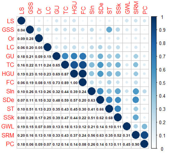
Figure 4.
Matrix of Cramer’s V. Three groups of highly correlated variables are present. Group 1: GU, TC, HGU, and FC; Group 2: SIn, SDe, ST, and SSk; and Group 3: SRM and PC. The variables are ordered according to the results of the agglomerative hierarchical clustering method.

Figure 5.
Dendrogram produced by agglomerative hierarchical clustering method for categorical variables.
- Group 1: geological units (GU), transmissivity coefficient (TC), hydrogeological units (HGU), and filtration coefficient (FC);
- Group 2: slope inclination (SIn), soil depth (SDe), soil type (ST), and soil skeleton (SSk);
- Group 3: surface relief morphology (SRM) and profil curvature (PC).
The first group consists of variables with a prevalence of hydrogeological characteristics. In this group, they have the highest association linkages: FC—HGU (1.00), FC—TC (0.89), TC—HGU (0.87), FC—GU (0.73), HGU—GU (0.69), and TC—GU (0.65). The rock complex in sandstone development is the main collector of groundwater, characterised by crack–intergrain permeability, and the drainage of this complex is considerably variable. These complexes are made by rocks with low permeability. Unlike this complex, rocks in sandstone-clay development are characterised by rhythmic alternation of sandstones and clay (or prevalence of sandstones in some parts of the formation), i.e., rocks with aquiferous properties with isolators that limit groundwater circulation in the complex. The clayey substrate is poorly permeable and most precipitation water flows over the surface, followed by more intensive erosion development (especially in deforested areas) with subsequent formation of landslips. The alternation of geological layers with different hydrogeological parameters in flysch areas represents a triggering factor for landslides during heavy rainfalls. In the second group are soil characteristics. The association linkages between variables are SSk—ST (0.68), SDe—ST (0.66), SDe—SIn (0.63), SSk—SDe (0.62), SSk—SIn (0.51), and ST—SIn (0.41). Landslide processes often arise due to the saturation of soil pores with water at deeper soils and the action of gravitational forces on unstable slopes (e.g., during long-term rains or as a result of snow melting). In the third group are relief characteristics. The two variables show very high association linkage SRM—PC (0.90). It is a connection of transport slope and linear relief curvature.
Variables—inclination of the slope, transmissivity coefficient, filtration coefficient, groundwater level, soil depth, and soil skeleton—are ordinal variables and for them, together with the continuous variable altitude, we have created the matrix of Spearman’s rank correlation coefficients (Figure 6). The values obtained confirm the findings of association between transmissivity coefficient—filtration coefficient (0.82), and soil depth—soil skeleton (−0.72) based on the values of Cramer’s V. In addition, the Spearman’s rank correlation coefficient gives the nature of the association based on whether the value is positive or negative: pixels with higher transmissivity coefficient usually also have higher filtration coefficient, whereas pixels with bigger soil depth usually have lower soil skeleton.
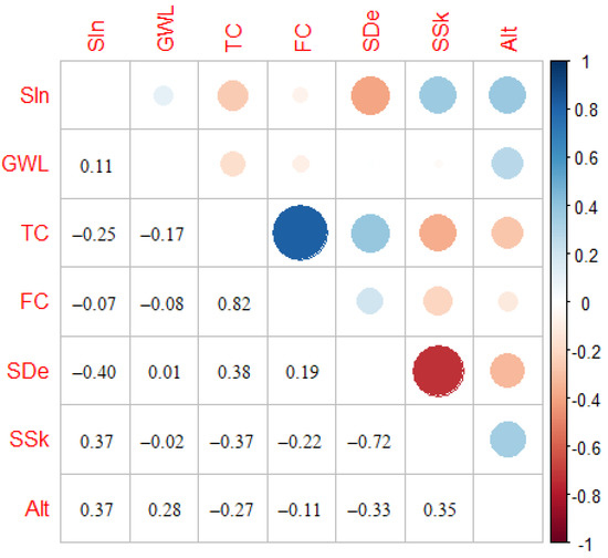
Figure 6.
Matrix of Spearman’s rank correlation coefficients.
4.2. Landslide Susceptibility Modelling
4.2.1. Logistic Regression
The presence of correlated variables in the logistic regression may negatively impact the training process and hinder the interpretability of the estimated coefficients [83]. Therefore, the selection of one variable from the groups identified in the previous section was performed first in the following manner. Using 5-fold cross-validation with balanced training datasets a simple logistic regression model with only one prediction variable was trained for each of the candidate variables and average AUC and Brier score values for both training ( and ) and validating ( and ) datasets were computed (Table 3). After taking into consideration the computed AUC and Brier score values, association with the other variables, and also the interpretability of the variables, we chose the following as the representatives of the three groups of variables showing association. From the first group, geological units were chosen since the AUC values were highest and Brier score values were almost as good as values for the hydrogeological units. In the second group, the soil type achieved the best values and was chosen. From the third group, profile curvature was chosen despite its slightly lower values than those for surface relief morphology because the difference is not large and profile curvature exhibits lower association with other variables.
Table 3.
Average values of AUC and Brier score on training and validating datasets for associated variables. Standard deviation is given in parentheses. Variables selected for the logistic regression model are highlighted in green.
The logistic regression model with predictor variables geological units, profile curvature, soil type, grain-size of soils, orientation, land cover, groundwater level, and altitude was then trained and its performance evaluated using 5-fold cross-validation with two different types of training datasets as described in Section 3.4.
The computed average values of the selected metrics for evaluating the classification performance and calibrating predicted probabilities are summarised in Table 4. The average values of for both stratified and balanced training datasets were approximately the same — , which according to the work in [83] is acceptable, albeit not very high. The average values of other considered classification measures computed on the validation datasets were also very close for both types of training datasets. The higher average accuracy and values as well as significantly lower average value of on the validation dataset than on the balanced training dataset are probably the consequence of a higher ratio of non-landslide pixels in the validation dataset. The average values of stratified Brier scores show that model trained on balanced datasets achieved similar scores for both landslide and non-landslide pixels, while the model trained on the stratified datasets greatly favours non-landslide pixels at the expense of landslide pixels, as is evident from the high values on landslide pixels and very low values on non-landslide pixels. The overall Brier score was better for stratified datasets, however, this is because almost 87% of all pixels are non-landslide. The computed average values of the considered measures achieved on training datasets are also reported for completeness.
Table 4.
Average values of metrics based on classification performance of (, , , , and ) and calibration of probabilities () by logistic regression and random forest models. Bar indicates the average value of metric and standard deviation is given in parentheses. Note that for lower values indicate better performance.
4.2.2. Random Forests
To find the number of variables considered for the splitting condition randomly chosen from all 15 input variables for each node separately, , that optimises the random forests model performance, models with varying from 1 to 15 were trained and their performance in terms of the AUC and the overall Brier score was evaluated using 5-fold cross-validation with balanced datasets (Figure 7). The highest average value of was achieved for and the lowest average value of was achieved for . Therefore, the selected value of used for computing other performance measures and producing a landslide susceptibility map was 8.
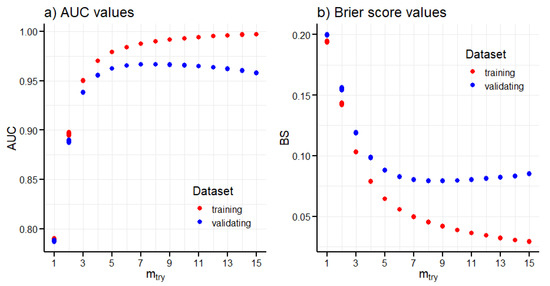
Figure 7.
Values of AUC (a) and overall Brier score (b) for different values of . Values for each model trained during the 5-fold cross-validation were plotted separately.
The computed average values of the selected metrics for evaluating the classification performance and calibrating predicted probabilities for the random forests model with and are summarised in Table 4. The average values of were close for both balanced and stratified training datasets and were exceptionally high, and for balanced and stratified datasets, respectively. For the other classification measures considered, models trained on stratified datasets performed slightly better, except for true positive rate . Again, the higher average value and the significantly lower average value on the validation dataset than on the balanced training dataset are probably the consequence of a higher ratio of non-landslide pixels in the validation dataset. The better average value of the overall Brier score was achieved by the model trained on the stratified datasets. The average values of stratified Brier scores indicate that training on the stratified datasets puts more weight on the non-landslide pixels as can be expected due to them representing a majority in the datasets while training on the balanced datasets puts more weight on the landslide pixels. The computed average values of the considered measures achieved on training datasets are also reported for completeness.
As random forest models show a very good ability to distinguish between landslide and non-landslide pixels, the significance of the variables used in the model was evaluated using the permutation importance measure [80]. The results are shown in Figure 8. Altitude was found to be the most significant variable, followed by orientation and groundwater level. Orientation plays an important role in the climatic factors of the area. The area is rich in atmospheric precipitation, which is due to its greater exposure to the prevailing northwestern current. It is part of a wider area lying at the interface of oceanic and continental influences, where air masses of various properties alternate several times during the year. Ocean currents reduce the differences between summer and winter (winters are warmer and summers are colder), causing more cloud cover, more rainfall, and more frequent fogging. Changes in the groundwater level can cause landslides, especially in the vicinity of watercourses (this is mainly the fluctuation of the groundwater level in spring or autumn). Geological structure, geomorphological conditions and character of georelief and related hydrogeological conditions of the area as well as anthropogenic factors represented by landscape structure and land use can also be considered relevant variables that reflect favourable conditions for landslides.
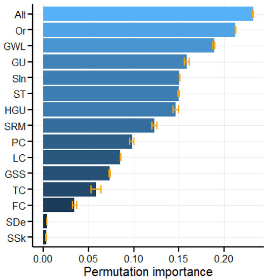
Figure 8.
The average permutation importance of variables. Bars indicate standard deviation of the permutation importance across the 5 folds of the cross-validation.
4.2.3. Comparison of the Models
The type of training datasets has very little effect on the classification performance on the validation datasets for both the logistic regression and the random forest models, with logistic regression displaying smaller differences. The random forest model outperformed the logistic regression model in all considered measures, achieving very good values of , , and when trained on balanced datasets compared to values achieved by the logistic regression model—, , and . Although the random forest model is better at correctly classifying landslide pixels with its value of than the logistic regression model with its value of , the comparison with the very good ability to correctly classify non-landslide pixels () indicates room for improvement.
The logistic regression model used in this study achieved similar performance, based on values, as models used in several studies, e.g., [91] (), [92] (), [6] (), and [93] (), while others report higher values, e.g., [94] (), [95] (), and [96] (the highest reported value was ). The random forest model achieved a very high average value of , which is in agreement with several studies that reported similar values, e.g., [97] (), [48] (), [98] (), and [99] (), while others report lower values, e.g., [91] (), [46] (), and [6] (). The observed viability in model performance reported in the literature may be due to the different methods used in data preparation for model training, e.g., mapping units used (pixels, polygons, slope units), number of data points representing landslides (single point or multiple), and handling of categorical conditioning factors (as dummy variables or transformation into continuous variables). The study performed in [96], where the authors used logistic regression to model landslide susceptibility in four different areas and reported values of between 0.851 and 0.940, suggests that there is also some inherent variability in the effect of conditioning factors on landslide susceptibility. The finding that the random forest model achieves better performance at the task of landslide susceptibility modelling presented in this study is in agreement with studies [6,91,93], where a comparison between the logistic regression models and random forest model was also performed.
A common practice in landslide susceptibility modelling is to immediately convert probabilities predicted by the models to sensitivity classes using Jenks natural breaks method. As this method automatically selects sensitivity ranges based on the input data, it can obscure poor calibration of predicted probabilities which are an important output of the susceptibility models.
As is evident from the average values of stratified Brier scores, the training dataset composition has an impact on the predicted probabilities which can be illustrated by creating histograms of these probabilities (Figure 9). Logistic regression predicted low probabilities when trained on stratified training datasets compared to balanced training datasets (Figure 9a,b), severely underestimating the probability of landslide occurrence even for the landslide pixels. If the Jenks natural breaks method was used before assessing the predicted probabilities, distinguishing which model is better would be difficult, even though the one trained on the stratified datasets predicts probabilities of landslide occurrence below 0.5 for the majority of landslide pixels. A similar instance of a model underestimating landslide occurrence probability can be seen in [100], where the upper bound of the very high susceptibility class is 0.5.
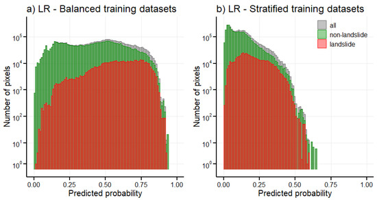
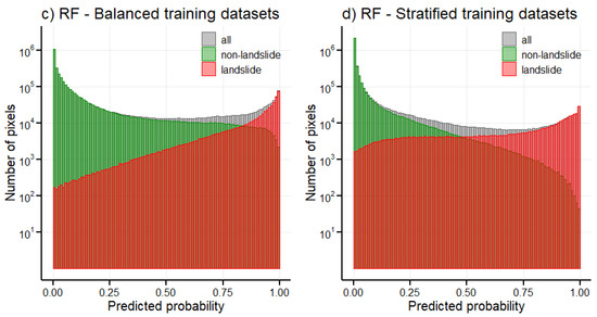
Figure 9.
Histograms of predicted landslide susceptibility probabilities by logistic regression (LR; (a,b)) and random forest (RF; (c,d)) models trained on different types of datasets for different types of pixels—for all pixels in the background, for landslide pixels in the forefront, and for non-landslide pixels in the middle. Predicted probabilities for individual testing datasets from cross-validation were combined to create one dataset. Note the logarithmic scale on the vertical axes.
With the random forest models, the predicted probabilities cover the whole interval for both types of datasets (Figure 9c,d), although their effect can be seen in plateauing of the histograms for predicted probabilities for landslide (red histogram in Figure 9c) and non-landslide (green histogram in Figure 9d) pixels for stratified and balanced training datasets, respectively. Histograms of probabilities predicted by random forest models (Figure 9c,d) indicate that depending on the application and which type of pixels are more important to correctly classify, using a balanced training dataset might result in better performance.
Furthermore, these histograms provide us with insights into why the random forest model greatly outperformed the logistic regression model. For the random forest model the distribution of predicted probabilities for all pixels (grey histograms in Figure 9c,d) exhibits a pronounced U-shape and histograms for landslide and non-landslide pixels (red and green histograms in Figure 9c,d) are very different, as could be expected from a well performing classification model. On the other hand, for the logistic regression model the histograms for landslide and non-landslide pixels (red and green histograms in Figure 9a,b) are very similar to each other.
4.3. Landslide Susceptibility Mapping
A standard result of the landslide susceptibility modelling is the map showing spatial distribution of the predicted probabilities. To create such a map, logistic regression and random forest models trained on balanced datasets were used and for each model the predicted probabilities for individual validation datasets from cross-validation were aggregated to create an overall validation dataset. These datasets were then used to create landslide susceptibility maps (Figure 10).
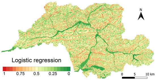
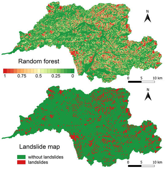
Figure 10.
Visualisation of the landslide susceptibility maps based on the probabilities predicted by logistic regression and random forests models and the map of landslide inventory used.
To simplify interpreting the resulting susceptibility map, the predicted probabilities from the logistic regression and the random forest models were divided into six categories of landslide susceptibility: no susceptibility [0, 0.01), very low susceptibility [0.01, 0.2), low susceptibility [0.2, 0.4), moderate susceptibility [0.4, 0.6), high susceptibility [0.6, 0.8), and very high susceptibility [0.8, 1].
According to the logistic regression model, only 0.018% of the Kysuce region was classified as without susceptibility to landslides. According to the random forests model, it was up to 24.8%. For the logistic regression model, the slopes with very low susceptibility cover 17.2% of the area while for the random forests model it is 40.6% of the area. The slopes with very high susceptibility cover 2.6% of the area for the logistic regression model and 12.7% of the area for the random forests model (Figure 11). When compared with currently registered landslides that cover 18.26% of the area (1869 landslides), the random forests model appears to be more realistic. Furthermore, compare the map results in Figure 10.
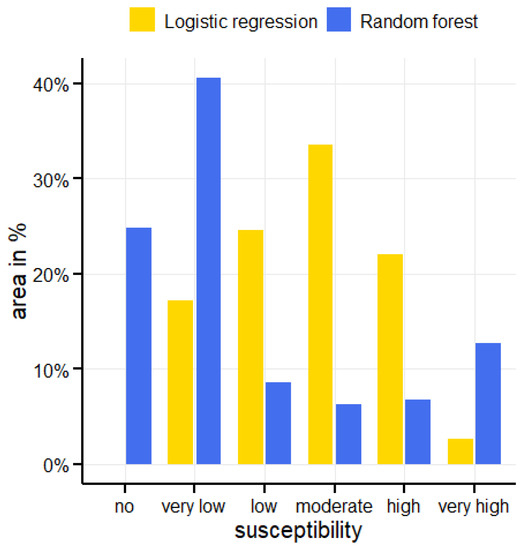
Figure 11.
The representation of categories of landslide susceptibility of the area according to models of logistic regression and random forests.
The probability of landslide occurrence according to the random forest model is the highest on pixels with soil consisting of deluvial sediments or possibly sandy flysch, which are characterised as permeable rocks with middle transmissivity, and groundwater level spanning below the surface covered by coniferous forests or meadows and grasslands on a transport slope with linear curvature at an inclination from to that is oriented mostly towards south, southeast, west and southwest. The probability of landslide occurrence according to the logistic regression model is the highest on pixels with soil consisting of deluvial sediments (permeable rocks with medium flow) and groundwater level spanning below the surface covered by non-forest woody vegetation or coniferous forests on a slope depression with concave curvature at an inclination from to that is oriented mostly towards south, southwest, west, and northwest.
5. Conclusions
Our paper represents a study of the selected landslide hazard in the landscape evaluated by two statistical predictive methods (the logistic regression method and the random forests method). The results show that (based on Cramer’s V correlation matrix) three groups of variables seem to be highly correlated. Based on Spearman’s rank correlation coefficient computed for categorical ordinal variables, the high correlation between the variables (transmissivity coefficient—filtration coefficient, the depth of soil—soil skeleton) was confirmed.
The geological–substrate complex, horizontal form of the relief, and soil type were chosen as the representative variables from the variables in groups in the logistic regression model. The model trained on the balanced datasets achieved values of , , , , , and , which indicate that logistic regression is ill equipped for such a complex task as landslide susceptibility modelling.
The random forest model trained on balanced datasets vastly outperformed the logistic regression model and achieved very good values on all performance metrics considered: , , , , , and . Altitude, orientation, and depth of groundwater emerged as some of the more significant variables in building the random forest model.
The results presented in this study show that while the training dataset type (stratified or balanced) has little impact on the classification performance of the logistic regression model; it has great impact on the predicted landslide susceptibility probabilities, with balanced training datasets producing probabilities that are less likely to underestimate landslide occurrence. With the random forest model the training dataset composition influences on which pixel type more weight is put, however, the effect on the predicted probabilities is mild. The results produced by the logistic regression model clearly indicate the need to incorporate usage of metrics such as Brier score into the landslide susceptibility modelling methodology.
Due to gradual urbanization and increasing desire for higher quality of life, the architects are forced to inquire into evaluating complex engineer-geological relations in more detail when assessing land, underground, linear, water, and other types of buildings.
An important condition is a detailed knowledge of the current state of the geological environment, geo-barriers, terrain characteristics, and other components of the natural environment. Predicting geological processes that can take place in the future in the given area is a necessity as well. Here, modelling the characteristics of the area and objectively assessing possibilities or conditions of area usage are of great benefit. Determining optimal conditions for area usage and appropriate construction location in the area can be means of reducing high expenses on possible future reconstruction and, last but not least, increasing the safety of the inhabitants.
Author Contributions
Conceptualization, M.B. and P.B.; methodology, M.B., M.Š. and P.B.J.; software, M.Š. and P.B.J.; validation, M.B. and P.B.J.; formal analysis, M.B., P.B.J. and P.B.; investigation, M.B., P.B.J. and P.B.; resources, M.B. and P.B.J.; data curation, M.B.; writing-original draft preparation, M.B., P.B.J., P.B. and M.Š.; writing-review and editing, M.B. and P.B.J.; visualization, P.B., P.B.J. and M.Š.; supervision, M.B. and P.B. All authors have read and agreed to the published version of the manuscript.
Funding
This work was supported by the Projects: VEGA Historical and present changes in the landscape diversity and biodiversity caused by natural and anthropogenic under Grant 2/0132/18.
Institutional Review Board Statement
Not applicable.
Informed Consent Statement
Not applicable.
Data Availability Statement
Not applicable.
Acknowledgments
We are grateful to Zuzana Molnárová for English proofreading.
Conflicts of Interest
The authors declare no conflict of interest.
References
- Nemčok, A. Zosuvy v Slovenských Karpatoch; VEDA: Bratislava, Slovakia, 1982. [Google Scholar]
- Catani, F.; Lagomarsino, D.; Segoni, S.; Tofani, V. Landslide susceptibility estimation by random forests technique: Sensitivity and scaling issues. Nat. Hazards Earth Syst. Sci. 2013, 13, 2815–2831. [Google Scholar] [CrossRef]
- Brabb, E. Innovative approaches to landslide hazard mapping. In Proceedings of the 4th International Symposium on Landslides, Toronto, ON, Canada, 16–21 September 1984; pp. 307–324. [Google Scholar]
- Remondo, J.; González, A.; De Terán, J.; Cendrero, A.; Fabbri, A.; Chung, C. Validation of Landslide Susceptibility Maps; Examples and Applications from a Case Study in Northern Spain. Nat. Hazards 2003, 30, 437–449. [Google Scholar] [CrossRef]
- Glade, T.; Crozier, M.J. A review of scale dependency in landslide hazard and risk analysis. Landslide Hazard Risk 2005, 75, 75–138. [Google Scholar]
- Youssef, A.; Pourghasemi, H.; Pourtaghi, Z.; Al-Katheeri, M. Landslide susceptibility mapping using random forest, boosted regression tree, classification and regression tree, and general linear models and comparison of their performance at Wadi Tayyah Basin, Asir Region, Saudi Arabia. Landslides 2016, 13, 839–856. [Google Scholar] [CrossRef]
- Yilmaz, I. Landslide susceptibility mapping using frequency ratio, logistic regression, artificial neural networks and their comparison: A case study from Kat landslides (Tokat—Turkey). Comput. Geosci. 2009, 35, 1125–1138. [Google Scholar] [CrossRef]
- Guzzetti, F.; Carrara, A.; Cardinali, M.; Reichenbach, P. Landslide hazard evaluation: A review of current techniques and their application in a multi-scale study, Central Italy. Geomorphology 1999, 31, 181–216. [Google Scholar] [CrossRef]
- Glade, T.; Anderson, M.G.; Crozier, M. Landslide Hazard and Risk; John Wiley and Sons, Ltd.: Chichester, UK, 2005. [Google Scholar]
- Dou, J.; Bui, D.T.; Yunus, A.P.; Jia, K.; Song, X.; Revhaug, I.; Xia, H.; Zhu, Z. Optimization of causative factors for landslide susceptibility evaluation using remote sensing and GIS data in parts of Niigata, Japan. PLoS ONE 2015, 10, e0133262. [Google Scholar]
- Chen, T.; Niu, R.; Jia, X. A comparison of information value and logistic regression models in landslide susceptibility mapping by using GIS. Environ. Earth Sci. 2016, 75, 867. [Google Scholar] [CrossRef]
- Tsangaratos, P.; Ilia, I.; Hong, H.; Chen, W.; Xu, C. Applying Information Theory and GIS-based quantitative methods to produce landslide susceptibility maps in Nancheng County, China. Landslides 2017, 14, 1091–1111. [Google Scholar] [CrossRef]
- Shirzadi, A.; Soliamani, K.; Habibnejhad, M.; Kavian, A.; Chapi, K.; Shahabi, H.; Chen, W.; Khosravi, K.; Thai Pham, B.; Pradhan, B.; et al. Novel GIS Based Machine Learning Algorithms for Shallow Landslide Susceptibility Mapping. Sensors 2018, 18, 3777. [Google Scholar] [CrossRef]
- Chen, W.; Shahabi, H.; Zhang, S.; Khosravi, K.; Shirzadi, A.; Chapi, K.; Pham, B.T.; Zhang, T.; Zhang, L.; Chai, H.; et al. Landslide Susceptibility Modeling Based on GIS and Novel Bagging-Based Kernel Logistic Regression. Appl. Sci. 2018, 8, 2540. [Google Scholar] [CrossRef]
- Nohani, E.; Moharrami, M.; Sharafi, S.; Khosravi, K.; Pradhan, B.; Pham, B.T.; Lee, S.; M. Melesse, A. Landslide Susceptibility Mapping Using Different GIS-Based Bivariate Models. Water 2019, 11, 1402. [Google Scholar] [CrossRef]
- Lei, X.; Chen, W.; Pham, B.T. Performance Evaluation of GIS-Based Artificial Intelligence Approaches for Landslide Susceptibility Modeling and Spatial Patterns Analysis. ISPRS Int. J. Geo-Inf. 2020, 9, 443. [Google Scholar] [CrossRef]
- Pradhan, A.; Kim, Y. Evaluation of a combined spatial multi-criteria evaluation model and deterministic model for landslide susceptibility mapping. Catena 2016, 140, 125–139. [Google Scholar] [CrossRef]
- Akgun, A.; Erkan, O. Landslide susceptibility mapping by geographical information system-based multivariate statistical and deterministic models: In an artificial reservoir area at Northern Turkey. Arab. J. Geosci. 2016, 9, 162. [Google Scholar] [CrossRef]
- Ciurleo, M.; Cascini, L.; Calvello, M. A comparison of statistical and deterministic methods for shallow landslide susceptibility zoning in clayey soils. Eng. Geol. 2017, 223, 71–81. [Google Scholar] [CrossRef]
- Canoğlu, M. Deterministic landslide susceptibility assessment with the use of a new index (factor of safety index) under dynamic soil saturation: An example from demirciköy watershed (Sinop/Turkey). Carpathian J. Earth Environ. Sci. 2017, 12, 423–436. [Google Scholar]
- Ayalew, L.; Yamagishi, H. The application of GIS-based logistic regression for landslide susceptibility mapping in the Kakuda-Yahiko Mountains, Central Japan. Geomorphology 2005, 65, 15–31. [Google Scholar] [CrossRef]
- Van Den Eeckhaut, M.; Vanwalleghem, T.; Poesen, J.; Govers, G.; Verstraeten, G.; Vandekerckhove, L. Prediction of landslide susceptibility using rare events logistic regression: A case-study in the Flemish Ardennes (Belgium). Geomorphology 2006, 76, 392–410. [Google Scholar] [CrossRef]
- Lin, L.; Lin, Q.; Wang, Y. Landslide susceptibility mapping on a global scale using the method of logistic regression. Nat. Hazards Earth Syst. Sci. 2017, 17, 1411–1424. [Google Scholar] [CrossRef]
- Raja, N.; Çiçek, I.; Türkoğlu, N.; Aydin, O.; Kawasaki, A. Landslide susceptibility mapping of the Sera River Basin using logistic regression model. Nat. Hazards 2017, 85, 1323–1346. [Google Scholar] [CrossRef]
- Lombardo, L.; Mai, P.M. Presenting logistic regression-based landslide susceptibility results. Eng. Geol. 2018, 244, 14–24. [Google Scholar] [CrossRef]
- Polykretis, C.; Chalkias, C. Comparison and evaluation of landslide susceptibility maps obtained from weight of evidence, logistic regression, and artificial neural network models. Nat. Hazards 2018, 93, 249–274. [Google Scholar] [CrossRef]
- Guzzetti, F.; Reichenbach, P.; Cardinali, M.; Galli, M.; Ardizzone, F. Probabilistic landslide hazard assessment at the basin scale. Geomorphology 2005, 72, 272–299. [Google Scholar] [CrossRef]
- Guzzetti, F.; Reichenbach, P.; Ardizzone, F.; Cardinali, M.; Galli, M. Estimating the quality of landslide susceptibility models. Geomorphology 2006, 81, 166–184. [Google Scholar] [CrossRef]
- Pham, B.T.; Prakash, I. Evaluation and comparison of LogitBoost Ensemble, Fisher’s Linear Discriminant Analysis, logistic regression and support vector machines methods for landslide susceptibility mapping. Geocarto Int. 2019, 34, 316–333. [Google Scholar] [CrossRef]
- Choubin, B.; Moradi, E.; Golshan, M.; Adamowski, J.; Sajedi-Hosseini, F.; Mosavi, A. An ensemble prediction of flood susceptibility using multivariate discriminant analysis, classification and regression trees, and support vector machines. Sci. Total Environ. 2019, 651, 2087–2096. [Google Scholar] [CrossRef]
- Wang, G.; Chen, X.; Chen, W. Spatial Prediction of Landslide Susceptibility Based on GIS and Discriminant Functions. ISPRS Int. J. Geo-Inf. 2020, 9, 144. [Google Scholar] [CrossRef]
- Falaschi, F.; Giacomelli, F.; Federici, P.; Puccinelli, A.; D’Amato Avanzi, G.; Pochini, A.; Ribolini, A. Logistic regression versus artificial neural networks: Landslide susceptibility evaluation in a sample area of the Serchio River valley, Italy. Nat. Hazards 2009, 50, 551–569. [Google Scholar] [CrossRef]
- Pradhan, B.; Lee, S. Landslide susceptibility assessment and factor effect analysis: Backpropagation artificial neural networks and their comparison with frequency ratio and bivariate logistic regression modelling. Environ. Model. Softw. 2010, 25, 747–759. [Google Scholar] [CrossRef]
- Pradhan, B. A comparative study on the predictive ability of the decision tree, support vector machine and neuro-fuzzy models in landslide susceptibility mapping using GIS. Comput. Geosci. 2013, 51, 350–365. [Google Scholar] [CrossRef]
- Lee, M.; Park, I.; Won, J.; Lee, S. Landslide hazard mapping considering rainfall probability in Inje, Korea. Geomat. Nat. Hazards Risk 2016, 7, 424–446. [Google Scholar] [CrossRef]
- Bragagnolo, L.; da Silva, R.V.; Grzybowski, J.M.V. Landslide susceptibility mapping with r. landslide: A free open-source GIS-integrated tool based on Artificial Neural Networks. Environ. Model. Softw. 2020, 123, 104565. [Google Scholar] [CrossRef]
- Zhu, A.X.; Wang, R.; Qiao, J.; Qin, C.Z.; Chen, Y.; Liu, J.; Du, F.; Lin, Y.; Zhu, T. An expert knowledge-based approach to landslide susceptibility mapping using GIS and fuzzy logic. Geomorphology 2014, 214, 128–138. [Google Scholar] [CrossRef]
- Shahabi, H.; Hashim, M.; Ahmad, B. Remote sensing and GIS-based landslide susceptibility mapping using frequency ratio, logistic regression, and fuzzy logic methods at the central Zab basin, Iran. Environ. Earth Sci. 2015, 73, 8647–8668. [Google Scholar] [CrossRef]
- Fatemi Aghda, S.; Bagheri, V.; Razifard, M. Landslide Susceptibility Mapping Using Fuzzy Logic System and Its Influences on Mainlines in Lashgarak Region, Tehran, Iran. Geotech. Geol. Eng. 2018, 36, 915–937. [Google Scholar] [CrossRef]
- Vahidnia, M.H.; Alesheikh, A.A.; Alimohammadi, A.; Hosseinali, F. A GIS-based neuro-fuzzy procedure for integrating knowledge and data in landslide susceptibility mapping. Comput. Geosci. 2010, 36, 1101–1114. [Google Scholar] [CrossRef]
- Chen, W.; Panahi, M.; Tsangaratos, P.; Shahabi, H.; Ilia, I.; Panahi, S.; Li, S.; Jaafari, A.; Ahmad, B.B. Applying population-based evolutionary algorithms and a neuro-fuzzy system for modeling landslide susceptibility. Catena 2019, 172, 212–231. [Google Scholar] [CrossRef]
- Marjanović, M.; Kovačević, M.; Bajat, B.; Voženílek, V. Landslide susceptibility assessment using SVM machine learning algorithm. Eng. Geol. 2011, 123, 225–234. [Google Scholar] [CrossRef]
- Hong, H.; Pradhan, B.; Xu, C.; Bui, D. Spatial prediction of landslide hazard at the Yihuang area (China) using two-class kernel logistic regression, alternating decision tree and support vector machines. Catena 2015, 133, 266–281. [Google Scholar] [CrossRef]
- Huang, Y.; Zhao, L. Review on landslide susceptibility mapping using support vector machines. Catena 2018, 165, 520–529. [Google Scholar] [CrossRef]
- Pourghasemi, H.; Kerle, N. Random forests and evidential belief function-based landslide susceptibility assessment in Western Mazandaran Province, Iran. Environ. Earth Sci. 2016, 75, 185. [Google Scholar] [CrossRef]
- Chen, W.; Xie, X.; Wang, J.; Pradhan, B.; Hong, H.; Bui, D.T.; Duan, Z.; Ma, J. A comparative study of logistic model tree, random forest, and classification and regression tree models for spatial prediction of landslide susceptibility. Catena 2017, 151, 147–160. [Google Scholar] [CrossRef]
- Taalab, K.; Cheng, T.; Zhang, Y. Mapping landslide susceptibility and types using Random Forest. Big Earth Data 2018, 2, 159–178. [Google Scholar] [CrossRef]
- de Oliveira, G.G.; Ruiz, L.F.C.; Guasselli, L.A.; Haetinger, C. Random forest and artificial neural networks in landslide susceptibility modeling: A case study of the Fão River Basin, Southern Brazil. Nat. Hazards 2019, 99, 1049–1073. [Google Scholar] [CrossRef]
- Pauditš, P.; Vlčko, J.; Jurko, J. Statistic methods in landslide hazard assessment. Miner. Slovaca 2005, 37, 529–538. [Google Scholar]
- Bednarik, M.; Magulová, B.; Matys, M.; Marschalko, M. Landslide susceptibility assessment of the Kral’ovany–Liptovskỳ Mikuláš railway case study. Phys. Chem. Earth Parts A/B/C 2010, 35, 162–171. [Google Scholar] [CrossRef]
- Havlín, A.; Bednarik, M.; Magulová, B.; Vlčko, J. Application of logistic regression for landslide susceptibility assessment in the middle part of Chriby Mts. (Czech Republik). Acta Geol. Slovaca 2011, 3, 153–161. [Google Scholar]
- Barančoková, M.; Kenderessy, P. Assessment of landslide risk using GIS and statistical methods in Kysuce region. Ekológia 2014, 33, 26–35. [Google Scholar] [CrossRef][Green Version]
- Muňko, M. Usability of Support Vector Machines Method in Prediction Modelling in GIS. Master’s Thesis, Slovak University of Technology in Bratislava, Bratislava, Slovakia, 2015. [Google Scholar]
- Mazúr, E.; Lukniš, M.; Geomorphological Units. In Atlas SSR. Slovak Academy of Sciences—Slovak Office of Geodesy and Cartography, IV Surface, Map 16, Scale 1:500,000 (in Slovak) 1980, 54–55. Available online: https://en-academic.com/dic.nsf/enwiki/7988647 (accessed on 1 December 2021).
- Mahel’, M. Geologická Stavba Československých Karpát: Paleoalpínske Jednotky; VEDA: Bratislava, Slovakia, 1986. [Google Scholar]
- Hók, J.; Šujan, M.; Šipka, F. Tektonické členenie Západnỳch Karpát–prehl’ad názorov a novỳ prístup. Acta Geol. Slovaca 2014, 6, 135–143. [Google Scholar]
- Šimeková, J.; Martinčeková, T.; Abrahám, P.; Gejdoš, T.; Grenčíková, A.; Grman, D. Atlas Máp Stability Svahov SR v Mierke 1:50,000. Záverečná Správa; Geofond, MŽP SR: Bratislava, Slovakia, 2006. [Google Scholar]
- Chen, W.; Zhang, S.; Li, R.; Shahabi, H. Performance evaluation of the GIS-based data mining techniques of best-first decision tree, random forest, and naïve Bayes tree for landslide susceptibility modeling. Sci. Total Environ. 2018, 644, 1006–1018. [Google Scholar] [CrossRef] [PubMed]
- Pauk, J.; Švec, P.; Hudec, A.; Babiak, K.; Draškovič, M. Renovation and Construction of Technical Infrastructure for Research and Development of the Institute of Landscape Ecology of the Slavak Academy of Sciences. Spatial Database System. Esprit Spol. s r.o., ÚKE SAV, Bratislava, Slovakia (in Slovak). 2013. Available online: https://www.researchgate.net/publication/322696745_Historicke_struktury_polnohospodarskej_krajiny_Slovenska_Historical_structures_of_the_agricultural_landscape_of_Slovakia (accessed on 1 December 2021).
- Van Westen, C.J.; Castellanos, E.; Kuriakose, S.L. Spatial data for landslide susceptibility, hazard, and vulnerability assessment: An overview. Eng. Geol. 2008, 102, 112–131. [Google Scholar] [CrossRef]
- Tseng, C.M.; Lin, C.W.; Hsieh, W.D. Landslide susceptibility analysis by means of event-based multi-temporal landslide inventories. Nat. Hazards Earth Syst. Sci. Discuss. 2015, 3, 1137–1173. [Google Scholar]
- Ciampalini, A.; Raspini, F.; Lagomarsino, D.; Catani, F.; Casagli, N. Landslide susceptibility map refinement using PSInSAR data. Remote Sens. Environ. 2016, 184, 302–315. [Google Scholar] [CrossRef]
- Wiedenmann, J.; Rohn, J.; Moser, M. The relationship between the landslide frequency and hydrogeological aspects: A case study from a hilly region in Northern Bavaria (Germany). Environ. Earth Sci. 2016, 75, 609. [Google Scholar] [CrossRef]
- Safaei, M.; Omar, H.; Huat, B.K.; Yousof, Z.B. Relationship between Lithology Factor and landslide occurrence based on Information Value (IV) and Frequency Ratio (FR) approaches–Case study in North of Iran. Electron. J. Geotech. Eng. 2012, 17, 79–90. [Google Scholar]
- Wu, C.; Qiao, J. Relationship between landslides and lithology in the Three Gorges Reservoir area based on GIS and information value model. Front. For. China 2009, 4, 165–170. [Google Scholar] [CrossRef]
- Reichenbach, P.; Rossi, M.; Malamud, B.D.; Mihir, M.; Guzzetti, F. A review of statistically-based landslide susceptibility models. Earth-Sci. Rev. 2018, 180, 60–91. [Google Scholar] [CrossRef]
- Potfaj, M.; Maglay, J.; Šlepecký, T.; Tet’ák, F. Geologická Mapa Regiónu Kysúc 1:50,000; Štátny geologický ústav Dionýza Štúra: Bratislava, Slovakia, 2002. [Google Scholar]
- Burrough, P.; McDonell, R. Principle of Geographic Information Systems; Oxford University Press: Oxford, UK, 1998. [Google Scholar]
- Agresti, A. An Introduction to Categorical Data Analysis; John Wiley & Sons: Hoboken, NJ, USA, 2018. [Google Scholar]
- Dormann, C.F.; Elith, J.; Bacher, S.; Buchmann, C.; Carl, G.; Carré, G.; Marquéz, J.R.G.; Gruber, B.; Lafourcade, B.; Leitao, P.J.; et al. Collinearity: A review of methods to deal with it and a simulation study evaluating their performance. Ecography 2013, 36, 27–46. [Google Scholar] [CrossRef]
- James, G.; Witten, D.; Hastie, T.; Tibshirani, R. An Introduction to Statistical Learning: With Application in R; Springer: New York, NY, USA, 2013; Volume 112. [Google Scholar]
- Cox, D.R. The regression analysis of binary sequences. J. R. Stat. Soc. Ser. B 1958, 20, 215–232. [Google Scholar] [CrossRef]
- Budimir, M.; Atkinson, P.; Lewis, H. A systematic review of landslide probability mapping using logistic regression. Landslides 2015, 12, 419–436. [Google Scholar] [CrossRef]
- Agresti, A. Categorical Data Analysis; John Wiley & Sons: Hoboken, NJ, USA, 2003; Volume 482. [Google Scholar]
- Breiman, L. Random forests. Mach. Learn. 2001, 45, 5–32. [Google Scholar] [CrossRef]
- Probst, P.; Boulesteix, A.L. To tune or not to tune the number of trees in random forest. J. Mach. Learn. Res. 2017, 18, 6673–6690. [Google Scholar]
- Oshiro, T.M.; Perez, P.S.; Baranauskas, J.A. How many trees in a random forest? In International Workshop on Machine Learning and Data Mining in Pattern Recognition; Springer: Berlin/Heidelberg, Germany, 2012; pp. 154–168. [Google Scholar]
- Izenman, A.J. Modern Multivariate Statistical Techniques: Regression, Classification, and Manifold Learning; Springer: New York, NY, USA, 2008. [Google Scholar]
- Malley, J.D.; Kruppa, J.; Dasgupta, A.; Malley, K.G.; Ziegler, A. Probability machines. Methods Inf. Med. 2012, 51, 74–81. [Google Scholar] [CrossRef] [PubMed]
- Breiman, L.; Cutler, A. Manual—Setting up, Using, and Understanding Random Forests V4. 0. 2003. Available online: https://www.stat.berkeley.edu/~breiman/Using_random_forests_v4.0.pdf (accessed on 14 June 2021).
- Hastie, T.; Tibshirani, R.; Friedman, J. The Elements of Statistical Learning: Data Mining, Inference, and Prediction, 2nd ed.; Springer: New York, NY, USA, 2009. [Google Scholar]
- Chicco, D.; Jurman, G. The advantages of the Matthews correlation coefficient (MCC) over F1 score and accuracy in binary classification evaluation. BMC Genom. 2020, 21, 6. [Google Scholar] [CrossRef]
- Hosmer, D.W.; Lemeshow, S. Applied Logistic Regression; John Wiley & Sons: Hoboken, NJ, USA, 2000. [Google Scholar]
- Brier, G.W. Verification of forecasts expressed in terms of probability. Mon. Weather Rev. 1950, 78, 1–3. [Google Scholar] [CrossRef]
- Wallace, B.C.; Dahabreh, I.J. Improving class probability estimates for imbalanced data. Knowl. Inf. Syst. 2014, 41, 33–52. [Google Scholar] [CrossRef]
- R Core Team. R: A Language and Environment for Statistical Computing; R Foundation for Statistical Computing: Vienna, Austria, 2021. [Google Scholar]
- Mangiafico, S. Rcompanion: Functions to Support Extension Education Program Evaluation. In R Package Version 2.4.1. 2020. Available online: http://rcompanion.org/ (accessed on 20 May 2021).
- Wei, T.; Simko, V. R Package “Corrplot”: Visualization of a Correlation Matrix. (Version 0.89). Available online: https://github.com/taiyun/corrplot (accessed on 20 May 2021).
- Wright, M.N.; Ziegler, A. ranger: A Fast Implementation of Random Forests for High Dimensional Data in C++ and R. J. Stat. Softw. 2017, 77, 1–17. [Google Scholar] [CrossRef]
- Wickham, H. ggplot2: Elegant Graphics for Data Analysis; Springer: New York, NY, USA, 2016. [Google Scholar]
- Chen, W.; Sun, Z.; Han, J. Landslide susceptibility modeling using integrated ensemble weights of evidence with logistic regression and random forest models. Appl. Sci. 2019, 9, 171. [Google Scholar] [CrossRef]
- Samia, J.; Temme, A.; Bregt, A.K.; Wallinga, J.; Stuiver, J.; Guzzetti, F.; Ardizzone, F.; Rossi, M. Implementing landslide path dependency in landslide susceptibility modelling. Landslides 2018, 15, 2129–2144. [Google Scholar] [CrossRef]
- Sevgen, E.; Kocaman, S.; Nefeslioglu, H.A.; Gokceoglu, C. A novel performance assessment approach using photogrammetric techniques for landslide susceptibility mapping with logistic regression, ANN and random forest. Sensors 2019, 19, 3940. [Google Scholar] [CrossRef] [PubMed]
- Grozavu, A.; Mărgărint, M.C.; Patriche, C.V. Landslide susceptibility assessment in the Brăieşti-Sineşti sector of Iaşi cuesta. Carpathian J. Earth Environ. Sci. 2012, 7, 39–46. [Google Scholar]
- Steger, S.; Brenning, A.; Bell, R.; Glade, T. The propagation of inventory-based positional errors into statistical landslide susceptibility models. Nat. Hazards Earth Syst. Sci. 2016, 16, 2729–2745. [Google Scholar] [CrossRef]
- Mărgărint, M.; Grozavu, A.; Patriche, C. Assessing the spatial variability of coefficients of landslide predictors in different regions of Romania using logistic regression. Nat. Hazards Earth Syst. Sci. 2013, 13, 3339–3355. [Google Scholar] [CrossRef]
- Zhang, K.; Wu, X.; Niu, R.; Yang, K.; Zhao, L. The assessment of landslide susceptibility mapping using random forest and decision tree methods in the Three Gorges Reservoir area, China. Environ. Earth Sci. 2017, 76, 1–20. [Google Scholar] [CrossRef]
- Achour, Y.; Pourghasemi, H.R. How do machine learning techniques help in increasing accuracy of landslide susceptibility maps? Geosci. Front. 2020, 11, 871–883. [Google Scholar] [CrossRef]
- Dou, J.; Yunus, A.P.; Bui, D.T.; Merghadi, A.; Sahana, M.; Zhu, Z.; Chen, C.W.; Khosravi, K.; Yang, Y.; Pham, B.T. Assessment of advanced random forest and decision tree algorithms for modeling rainfall-induced landslide susceptibility in the Izu-Oshima Volcanic Island, Japan. Sci. Total Environ. 2019, 662, 332–346. [Google Scholar] [CrossRef]
- Nhu, V.H.; Shirzadi, A.; Shahabi, H.; Chen, W.; Clague, J.J.; Geertsema, M.; Jaafari, A.; Avand, M.; Miraki, S.; Talebpour Asl, D.; et al. Shallow landslide susceptibility mapping by random forest base classifier and its ensembles in a semi-arid region of Iran. Forests 2020, 11, 421. [Google Scholar] [CrossRef]
Publisher’s Note: MDPI stays neutral with regard to jurisdictional claims in published maps and institutional affiliations. |
© 2021 by the authors. Licensee MDPI, Basel, Switzerland. This article is an open access article distributed under the terms and conditions of the Creative Commons Attribution (CC BY) license (https://creativecommons.org/licenses/by/4.0/).