Article

Agricultural Land Suitability Assessment Using Satellite Remote Sensing-Derived Soil-Vegetation Indices

by
Rubaiya Binte Mostafiz
1,
Ryozo Noguchi
2 and
Tofael Ahamed
2,*
1
Graduate School of Life and Environmental Sciences, University of Tsukuba, Tsukuba 305-8572, Japan
2
Faculty of Life and Environmental Sciences, University of Tsukuba, Tsukuba 305-8572, Japan
*
Author to whom correspondence should be addressed.
Land 2021, 10(2), 223; https://doi.org/10.3390/land10020223
Submission received: 15 January 2021 / Revised: 17 February 2021 / Accepted: 19 February 2021 / Published: 23 February 2021

Abstract

:
Satellite remote sensing technologies have a high potential in applications for evaluating land conditions and can facilitate optimized planning for agricultural sectors. However, misinformed land selection decisions limit crop yields and increase production-related costs to farmers. Therefore, the purpose of this research was to develop a land suitability assessment system using satellite remote sensing-derived soil-vegetation indicators. A multicriteria decision analysis was conducted by integrating weighted linear combinations and fuzzy multicriteria analyses in a GIS platform for suitability assessment using the following eight criteria: elevation, slope, and LST vegetation indices (SAVI, ARVI, SARVI, MSAVI, and OSAVI). The relative priorities of the indicators were identified using a fuzzy expert system. Furthermore, the results of the land suitability assessment were evaluated by ground truthed yield data. In addition, a yield estimation method was developed using indices representing influential factors. The analysis utilizing equal weights showed that 43% of the land (1832 km2) was highly suitable, 41% of the land (1747 km2) was moderately suitable, and 10% of the land (426 km2) was marginally suitable for improved yield productions. Alternatively, expert knowledge was also considered, along with references, when using the fuzzy membership function; as a result, 48% of the land (2045 km2) was identified as being highly suitable; 39% of the land (2045 km2) was identified as being moderately suitable, and 7% of the land (298 km2) was identified as being marginally suitable. Additionally, 6% (256 km2) of the land was described as not suitable by both methods. Moreover, the yield estimation using SAVI (R2 = 77.3%), ARVI (R2 = 68.9%), SARVI (R2 = 71.1%), MSAVI (R2 = 74.5%) and OSAVI (R2 = 81.2%) showed a good predictive ability. Furthermore, the combined model using these five indices reported the highest accuracy (R2 = 0.839); this model was then applied to develop yield prediction maps for the corresponding years (2017–2020). This research suggests that satellite remote sensing methods in GIS platforms are an effective and convenient way for agricultural land-use planners and land policy makers to select suitable cultivable land areas with potential for increased agricultural production.

1. Introduction

Proper land-use planning is essential for enhancing agricultural production and ecological conservation and for the protection of biodiversity [1]. Inappropriate land management practices lead to a higher rate of soil erosion, a diminished crop production, a hindered productivity, and a deteriorated soil quality [2]. Therefore, land management focusing on suitability should be a key issue of research and policy development mainly due to its influence on crop production. The knowledge of local land conditions has become increasingly recognized for its importance in sustainable land management [3]. Farmers of local communities assess their farmland using consistent observations and collective experiences [4]. However, for rural communities, this knowledge is usually insufficient to understand the adequacy of suitable condition, management strategies, and land-use decisions.
In addition, many conventional techniques for earth monitoring applications require specific spectral features that are defined only for multispectral data such as deep learning, exploiting both temporal and cross-sensor dependencies and deep networks achieve much better performance than traditional methods [5,6]. Furthermore, innovative farming technologies incorporate biology with computers and device exchange-based smart agriculture become achieved in a structured farm management system. The high spatial imagery from remote sensing datasets may provide an aid to systematically consider issues associated with smart farming technology. Remote sensing methods support the formation of growth profiles of plants and temporal evolution scheme of soils over their developmental phases [7]. Remote sensing indices that incorporate environmental recovery factors are useful for tracing the development of crops, their interrelatedness, and the consequences of the variables of interest for crop development. Following this concern, the application of smart agriculture and satellite remote sensing-based soil-vegetation index evaluations for agricultural land condition assessments is the key target of this research. Therefore, land suitability assessments can be performed using the multicriteria decision method. Such evaluation provides information about specific land use potentials and constraints. The Multicriteria Decision Method (MCDM) becomes more suitable when incorporating geospatial references. In recent years, computing technologies combined with GIS have enabled geospatial references using MCDM-land suitability evaluations. Furthermore, the MCDM, combined with linear combination and fuzzy set theory, has the potential to reduce subjectivity in the assessment of results. Several approaches to the MCDM that utilize equal-weighted linear combinations or fuzzy membership systems have been applied to conduct land suitability evaluations [8,9,10,11]. In addition, for sustainable land resource management, the Food and Agricultural Organization (FAO) has proposed guidelines for land evaluation [12]. According to the guidelines, land is classified into four categories: highly suitable, moderately suitable, marginally suitable, and not suitable. Additionally, the equal-weighted linear combination-fuzzy overlay technique in the GIS platform has the capabilities needed to overcome these limitations by applying the required calorie ratio (FAO recommended) to prepare land suitability assessments for smart agricultural practices. However, there is a lack of datasets in some areas of developing regions where assessments of land suitability are really challenging. In addition, recent datasets of those geographic information system have limitation, especially land uses, drainage and lack of soil sampling information for soil nutrients in a distant time period.
It is worth mentioning that quick and accurate land suitability assessments can aid in the improvement of yield prediction models. Regarding the judgment of the prediction of yield using vegetation indices (VIs), it is the most straightforward approach to establishing empirical relationships between ground-based yield measures and Vis [13,14,15]. In this regard, satellite remote sensing technologies and GIS applications for monitoring crops have the potential to establish timely assessments of changes in the growth and development of crops on regional scales [16]. The yield prediction is also helpful for making decisions on regional food security policies and production inventories to understand the availability of field crop.
Additionally, local farmer’s perceptions and their assessment of land suitability can differ from scientific approaches due to the much broader contextual implications of the former and how they are often framed. This often results in differences in perceived problems and the require solutions [17]. In most cases, developing location specific descriptions by soil sampling and analysis is expensive and challenging. Following this concern, advanced and affordable smart satellite remote sensing multicriteria technologies that consider climate factors are required for land suitability and accuracy assessments.
Therefore, the purpose of this research is to develop a soil-vegetation intent land suitability assessment model based on multicriteria decision-making analysis to determine optimal land distributions according to soil-vegetation indices to ensure elevated productivity, and a yield prediction method was developed using vegetation indices. A methodology that can be applied across various countries is proposed to reduce the complexities of farmland evaluation practices.

2. Materials and Methods

The proposed method utilizes a GIS-based multicriteria analysis to develop a soil-vegetation index-associated suitability analysis by exploiting satellite remote sensing for land suitability assessment and consists of three major steps (Figure 1): the calculation of soil vegetation indices for land suitability mapping of diversified crops, regression analysis using ground truth yield data for validation, and the utilization of a yield prediction model to develop a yield map. ArcGIS 10.4® (ESRI, CA, USA) software was used for criteria aggregation, data preprocessing and calculation standardization, weight determination by an equal-weighted overlay, fuzzy membership function, fuzzy overlay, and raster calculation.

2.1. Study Area

The study area is located between 25°14′ and 26°02′ N latitudes and 88°22′ and 89°54′ E longitudes in the northern part of Bangladesh and has a total area of 8260 square kilometers. The study was conducted in the Dinajpur, Rangpur, Kurigram, and Gaibandha districts of the Rangpur Division where the inhabitants derive their livelihoods from agriculture (Figure 2). The area consists of 36 administrative units with an overall population of 11,498,000 [18]. The population is economically active in agriculture; nevertheless, agronomic land use is highly inconsistent due to climatic factors, soil property issues, water infiltration, environmental resources, and local socioeconomic conditions. Based on weather data, the minimum and maximum mean annual temperature varies between 8.47 °C and 36.3 °C. The annual average rainfall recorded is 7650–1233 mm, with a high humidity in the range of 41–77% [19]. The elevation ranges from 5 to 30 m above sea level.

2.2. Image Acquisition

Landsat 8 is the most recently launched Landsat satellite and carries the Operational Land Imager (OLI) and Thermal Infrared Sensor (TIRS) instruments. OLI collects data in the visible, near infrared, and shortwave infrared spectral bands and in a panchromatic band. These two sensors provide seasonal coverage of the global landmass at a spatial resolution of 30 m (visible, NIR, and SWIR), 100 m (thermal), and 15 m (panchromatic). The 100 m TIRS data are registered to the OLI dataset to create radiometrically, geometrically, and terrain-corrected 12-bit data products. Images were acquired from 2017 to 2020. In this study, all satellite data were downloaded from the United States Geological Survey (USGS). The image was acquired (less than 10% cloud cover) in growing stage of the specific crop cycle (dry season irrigated rice).

2.3. Digital Image Preprocessing

All satellite images were first processed by resampling the band resolution at 30 m and then mosaicked and masked. Subsequently, an algebraic raster operation and a radiometric calibration as well as geometric and atmospheric corrections were applied to the remote sensing images using ArcGIS 10.4®. Image acquisition was performed for each band. After that, all selected bands were converted to a 30 m resolution using a resampling technique to ensure a similar cell size and data uniformity. The average reflectance values were calculated for the study area in each band using the raster calculator tool to compensate for the spatial variability to minimize the bias. Three different blocks collected during related time periods were mosaicked to cover the large study area.

2.4. Criteria Aggregation for Land Fertility Assessment

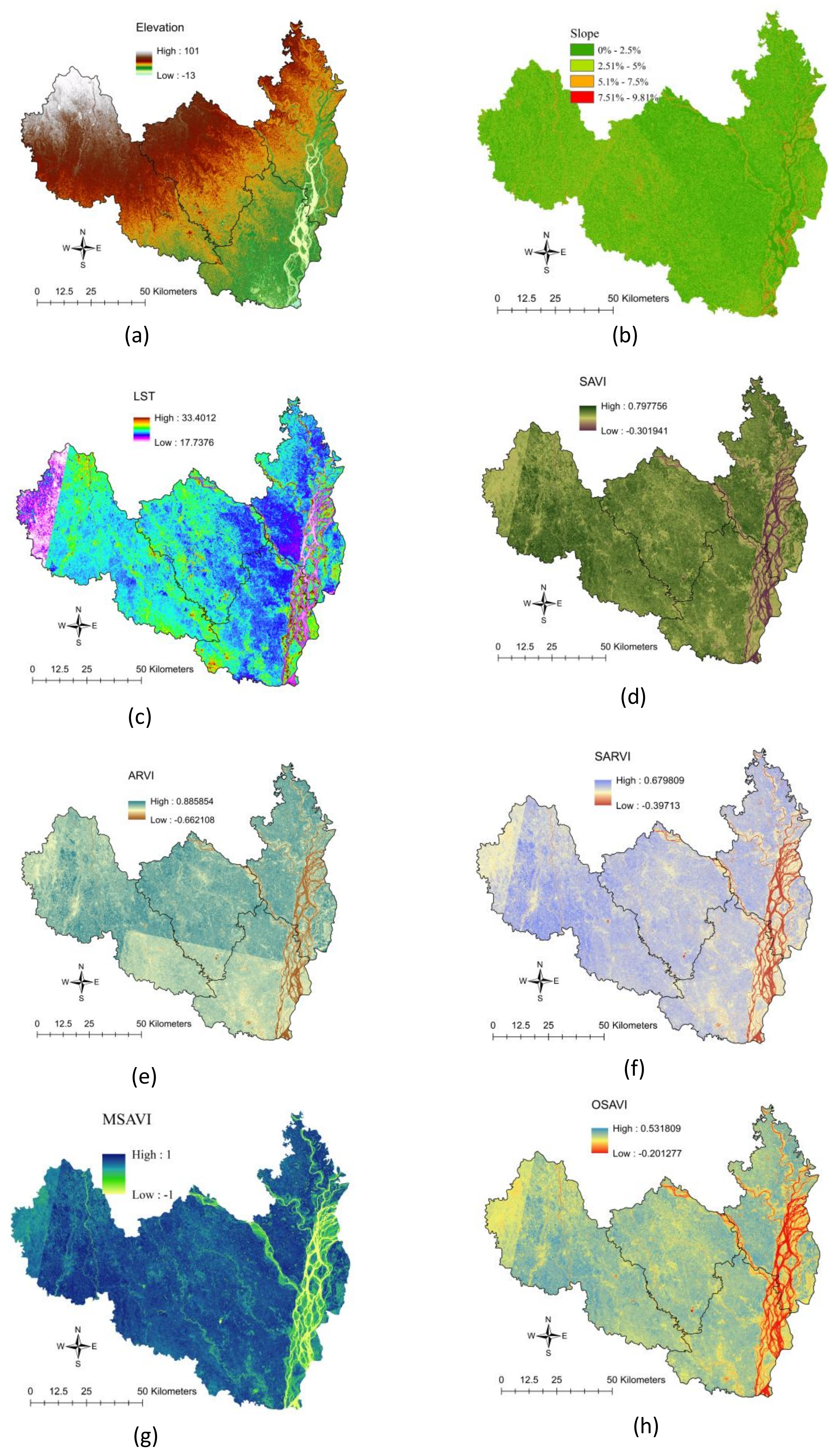
Three vital layers were developed by satellite data, and five vegetation indices were used as the input parameters to develop the land suitability analysis (Figure 3). The most important land and soil affiliated indices, SAVI, SARVI, ARVI, MASAVI, and OSAVI, were utilized to describe land conditions (Table 1). In addition, the slope and elevation layers were used as representative land conditions. The land surface temperature was taken as another influential criterion of agriculture land suitability assessment.

2.4.1. Elevation

Elevation is an important factor that plays a vital role in the variability of plant cover and causes temperature changes, particularly in highland areas. Areas with higher topographic elevations are more affected by rainfall and soil erosion [20]. Soil erosion is the alarming condition of agriculture field crop. Also, it is the main problems of agricultural development, such as landslides and flood events; these disasters have been severely influenced by the soil erosion process [21]. Most of the study area is plains land, and the elevation is less than 131 m (Figure 3a). The elevation data were extracted using a data elevation model (DEM) and were downscaled to a 30 m resolution.

2.4.2. Slope

Slope is a vital topographic element for indicating suitable farmland in assessments. Slope indicates many landscape processes, such as soil water content, erosion potential, runoff, and surface and subsurface flow velocity. The thickness of the soil layer decreases with the increasing slope [22]. The slope gradient has an impact on the runoff and soil loss: the greater the slope gradient the higher the potential for runoff and soil loss [23]. The slope was developed by using data from the original Shuttle Radar Topography Mission (SRTM) and the digital elevation model (DEM). The DEM was downscaled to a 30 m resolution. The Universal Transverse Mercator (UTM) projection system and WGS84 datum were used as rectifying agents in ArcGIS. The slope was calculated from the maximum rate of change between each cell and its neighbors. Every cell in the output raster had a slope value. Field crops generally require flat land; only a slight slope between 0% and 8% is resistant to erosion [24]. When the slope gradient is very steep (40%), soil sediment losses remain at the same high levels after cultivation abandonment because slope gradient is the main factor controlling soil erosion [25]. In the study area, the slope range was under 10% (Figure 3b), which is a suitable condition for most farming practices [26,27,28].

2.4.3. Land Surface Temperature (LST)

The LST (Figure 3c) was calculated for selected land areas using temporal information from Landsat 8 OLI images when less cloud coverage was present [29]. From 2017–2020, the LST data received from the obtained images ranged between 17 °C and 33 °C. The LST calculation was based on the moving average method. A single raster was formed from multiple years of raster datasets as the multiple predictions’ raster.
LST was calculated for the cropland using temporal information from Landsat 8 OLI that was selected during period of less cloud coverage. Two steps were required to calculate the LST; first, the NDVI was calculated for the given time period.
N D V I = ρ N I R ρ R E D ρ N I R + ρ R E D
After that, the resulting NDVI value was used to analyze the proportion vegetation (PV), which can be expressed as follows:
P V = N D V I N D V I m i n N D V I m a x N D V I m i n 2
After calculating the PV, the land surface emissivity (ελ) could be expressed as follows [30]:
ε λ = 0.004 P V + 0.986
Second, the thermal bands are included in band 10 and band 11 from the Landsat 8 imagery. The thermal bands were converted to digital numbers to estimate the radiance. The spectral radiance could be expressed as follows:
L λ = M L + Q C A L + A L L λ = 0.0003342 B a n d 10 + 0.1   a n d   L λ = 0.0003342 B a n d 11 + 0.1 L λ = 0.0003342 B a n d 10 + 0.1   a n d   L λ = 0.0003342 B a n d 11 + 0.1
where is the TOA spectral radiance at the sensor aperture, ML is the band-specific multiplicative rescaling factor from the metadata, QCAL is the quantized and calibrated standard product pixel value (DN), and AL is the band-specific additive rescaling factor from the metadata. Then, the brightness temperature (BT) could be expressed as follows (Jesus and Santana, 2017):
B T = K 2 ln K 1 L λ + 1 273.15
where BT is the satellite brightness temperature [Celsius]; K2 is the calibration constant 2 [Kelvin], where the band-specific thermal conversion constant is taken from the metadata; and K1 is the calibration constant 1 [Kelvin], where the band-specific thermal conversion constant is taken from the metadata. Finally, LST was calculated and expressed as follows [30]:
L S T = B T 1 + λ B T ρ ln ε λ
where λ is the average wavelength of band 10; ε λ is the emissivity calculated from Equation (3); and ρ is (h * c σ ), which is equal to 1.438 × 10⁻² mK, where σ is the Boltzmann constant (1.38 × 10⁻²³ J/K), h is Plank’s constant (6.626 × 10⁻³⁴ J.s) and c is the velocity of light (3 × 10⁸ m/s).

2.4.4. Soil-Adjusted Vegetation Index (SAVI)

Soil has a unique spectral signature that differs from that of other types of land cover. In the visible and near-infrared zones, reflectance increases in proportion to increases in wavelength. However, the rate of increase is affected by various factors. Soil moisture and organic matter may lower the soil reflectance. The association between red and near-infrared reflectance remains constant for different soil type physiognomies. When the moisture content changes, the two values are related and have a linear relationship. This relationship is very specific for each type of soil. SAVI is therefore useful for monitoring soils. Furthermore, SAVI is a modification of the normalized difference vegetation index (NDVI), which corrects for the influence of soil brightness when the vegetation cover is low [31]. SAVI (Figure 3d) was extracted from Landsat 8 OLI imagery by a mask for the study area. Datasets were acquired from 2017 to 2020. These datasets were used to build a single raster using map algebra in the ArcGIS platform.
To reduce the soil background effect, modified indices were proposed using the soil adjustment factor L to account for first-order soil background variations and obtain the SAVI [32]. SAVI can be expressed as follows:
S A V I = ρ N I R ρ R E D ρ N I R + ρ R E D + L 1 + L
where ρ N I R is the reflectance value in the near-infrared band, ρ R E D is the reflectance value in the red band, and L is the soil brightness correction factor. An L value of 0.5 in the reflectance space was found to minimize soil brightness variations and eliminate the need for additional calibration for different soils. The described SAVI value was 0.798 to −0.302 for the study area (Figure 3d).

2.4.5. Atmospherically Resistant Vegetation Index (ARVI)

The ARVI (Figure 3e) is obtained using a self-correction process for the atmospheric effect on the red channel, using the difference in the radiance between the blue and red channels to correct the radiance in the red channel due to the excellent atmospheric resistance of the ARVI [33].
A R V I = ρ N I R ρ R E D γ ρ B l U E ρ R E D ρ N I R + ( ρ R E D γ ρ B l U E ρ R E D )
where γ depends on the aerosol type. A good default value is γ = 1 when the aerosol model is not available. ARVI is resistant to atmospheric effects due to its self-correction process. This index uses the difference in the radiance between the blue and red bands to correct the radiance in the red band. Simulations show that ARVI has a similar dynamic range as SAVI, but on average, its sensitivity to atmospheric effects is four times less than that of NDVI [34]. The ARVI value fluctuated between 0.886 and −0.662 (Figure 3e).

2.4.6. Soil Adjusted and Atmospherically Resistant Vegetation Index (SARVI)

SARVI has a similar dynamic range to NDVI but is four times less sensitive to atmospheric effects than NDVI. SARVI performs much better for moderate to small sized aerosol particles (e.g., continental, urban, or smoke aerosol) than for large particles. Consequently, a single combination of blue and red channels in ARVI calculations may be used in all or most remote sensing applications [34].
S A R V I = 1 + L ρ N I R ρ R E D γ ( ρ B l U E ρ R E D ) / ρ N I R + ρ R E D γ ρ B l U E ρ R E D + L
where L is a correction factor similar to that in the SAVI calculation and γ is similar to that in the ARVI calculation. SARVI can minimize both canopy background and atmospheric effects [35,36]. In this research, the SARVI value was found to range from 0.679 to −0.397 (Figure 3f).

2.4.7. Modified Soil-Adjusted Vegetation Index (MSAVI)

Richardson and Wiegand (1977) proposed a modified secondary soil-adjusted vegetation index (MSAVI) [37], which can be expressed as follows:
M S A V I = 0.5 [ ( 2 ρ N I R + 1 ) 2 ρ N I R + 1 2 ( 8 ρ N I R ρ R E D ) ]
MSAVI does not rely on the soil line principle and has a simpler algorithm; it is mainly used in soil organic matter analysis, drought monitoring, and soil erosion analysis. In addition, it is useful for plant growth analyses, desertification studies, grassland yield estimations, and leaf area index (LAI) assessments. In the study area, the MSAVI value was observed to be between +1 and −1 (Figure 3g).

2.4.8. Optimized Soil-Adjusted Vegetation Index (OSAVI)

The Optimized Soil Adjusted Vegetation Index (OSAVI) is a newly developed alternative that can accommodate greater variability due to high soil background values [38]. OSAVI does not depend on the soil line and can eliminate the influence of the soil background effectively. However, the applications of OSAVI are not extensive; it is mainly used for the calculation of aboveground biomass, leaf nitrogen content, and chlorophyll content [39].
O S A V I = ρ N I R ρ R E D ρ N I R + ρ R E D + X
where X = 1.6. OSAVI is mainly used for the calculation of aboveground biomass, leaf nitrogen content, chlorophyll content, etc. The observed value was between 0.531 and −0.201 (Figure 3h).

2.5. Data Aggregation

2.5.1. Pattern Analysis

Several criteria were used for pattern analysis, which required pattern analyses from multiple years or months of data to form a predicted raster for reclassification. The single raster-based calculation was not reliable, nor did it provide enough datasets. This section shows several criteria from multiple years of data (2017 to 2020) for building a predicted raster for LST, SAVI, ARVI, SARVI, MSAVI, and OSAVI. The following section introduces the pattern analysis for multitemporal datasets into a single raster.

Moving Average

The moving average was processed after completing the digital image processing steps. The moving average was calculated in each year and can be expressed as follows:
M A n = i = 1 n D i n
where D is the number of data points in the raster cell and n is the amount of data to average.

Multiple Predicted Raster

As a part of the point pattern analysis, a single predicted raster was made. After that, LST, SAVI, ARVI, SARVI, MSAVI, and OSAVI were computed from 2017–2020. The basic extent encompassed the overall density pattern. This is basically the ratio of the observed number of single predicted rasters of points (r) to the study region area (a) and referred to as the multiple predicted raster (MPR). The MPR was applied as a criterion for land suitability analysis. MPR can be expressed as follows:
M P R = r a
where r is the ratio of the observed number of single predicted raster points and a is the area of the study region.

2.5.2. Land Use/Land Cover

Land use data enable the estimation of an area’s coverage with vegetated areas, settlements, forests, and water bodies. Land use data were collected from the Survey of Bangladesh (SoB), which was split into 92 blocks. After aggregation in the ArcGIS platform, the data were used to develop a more accurate land use/land cover (LULC) map for the land fertility assessment. In this study, rivers, forests, water bodies, and settlements were considered restrictions in the analysis. Subsequently, after excluding the constraints, only agricultural land was considered for land evaluation. Agricultural land was subclassified into cultivated land (80%), uncultivated land (0.5%) and vegetated land (19%) (Figure 2).

2.6. Land Fertility Assessment

The weighted overlay was used to prioritize the weights of each criterion to generate a land fertility assessment map. The reclassified raster data layers were combined with the weighted overlay in ArcGIS®. First, the combination criteria were input as equally weighted linear combinations. Second, the land suitability analysis was carried out by a fuzzy membership function, fuzzy reclassification and fuzzy overlay to evaluate the consistency of the two outcomes.

2.6.1. Map Development by Weighted-Linear Combination

First, reclassification was conducted to interpret the raster data by substituting a single value as the new value or by categorizing the ranges of values into a single value. Each criteria source map was reclassified into four classifications (Table 2). Land suitability analysis was conducted using different classification categories proposed by the FAO. As suggested by the FAO’s framework for land evaluation, the first class was designated as suitable (S) or not suitable (N). The suitability classification aimed to show the suitability of each land unit for crop production. In practice, three classes, namely (S1), (S2), and (S3), are typically used to identify land that is highly suitable, moderately suitable, and marginally suitable, respectively. The analysis was built using the aforementioned criteria and reclassified into 4 classes. Finally, the classes were found based on their weighted linear combination.
W e i g h t e d   O v e r l a y = i = 1 n C i W n
where Ci is each criterion (i) that has been reclassified and Wn is the number of data (n) that were weighted.

2.6.2. Map Development by the Fuzzy Membership Function

The fuzzification process had no sharply defined boundaries that characterized the imprecision of the classes. In this process, each value of the phenomenon central to the core of the definition of the set was set to 1. Those values that were not part of the set were set to 0. Those values that fell between these two extremes were within the transitional zone of the set, which was defined as the boundary [8,53,54,55]. In the present study, fuzzy membership classification was used to accommodate the high uncertainty of the scoring methods in assigning the suitability classes; several fuzzy membership functions were used for normalization. For this research, fuzzy functions were determined based on references and a literature review (Table 3).
Out of the seven varieties of fuzzy membership functions available, three fuzzy functions were used in this study considering ecological criteria: the fuzzy small, Gaussian, and fuzzy linear functions. These functions generate continuous fuzzy classifications under standardized criteria. The reclassification tool in ArcGIS enables the transformation of categorical data to range from 0 to 10 and then divides the resulting transformed data by 10 to derive a 0 to 1 scale. The equations for the fuzzy small (Equation (15)), fuzzy linear (Equation (16)), and Gaussian functions (Equation (17)) are as follows:
μ x = 1 1 + x f 2 f 1
The fuzzy small transformation function was used when small input values were more likely to be members of the set. The criterion slope was followed by a fuzzy small function in this research.
μ x = e ( f 1 x f 2 2 )
The layers of SAVI, ARVI, SARVI, MSAVI, and OSAVI were each followed by a fuzzy linear transformation function that related a linear function between the user-specified minimum and maximum values for reclassification.
μ x = f x = 0 x a b a 1 x a   a < x < b x b
The fuzzy Gaussian function converts the primal values into a normal distribution. If the input values decrease in membership, they move away from the midpoint. The midpoint of the fuzzy Gaussian function was set to 1 [59]. The elevation and LST layers were analyzed under the fuzzy Gaussian membership function.
In the fuzzy small and fuzzy linear membership functions, the control point included a midpoint (f2) and a spread (f1). The midpoint was a specific point that had a 0.5 value of membership in the large and small functions. Gaussian functions are determined by the user based in the references (ESRI, CA, USA). The spread was generally allocated a number between 1 and 10. The fuzzy membership curve became steeper for higher spread values. The fuzzy linear transformation function applied a linear function between the minimum and maximum values. Any value below the minimum was determined to be 0 (not a member), and any value above the maximum was 1 (a member) [61]. To analyze the relationships and interactions between all the sets for the 8 criteria in the overlay model, fuzzy overlay techniques were used. The available fuzzy set overlay techniques in ArcGIS are fuzzy And, fuzzy Or, fuzzy Product, fuzzy Sum, and fuzzy Gamma. Each of these techniques described the cell’s membership related to the input sets. In this study, the fuzzy Gamma overlay assisted in developing suitability maps for three identical seasons, which were determined based on references and a literature review (ESRI, Redlands, CA, USA).

2.7. Validation Using Ground Truth Data

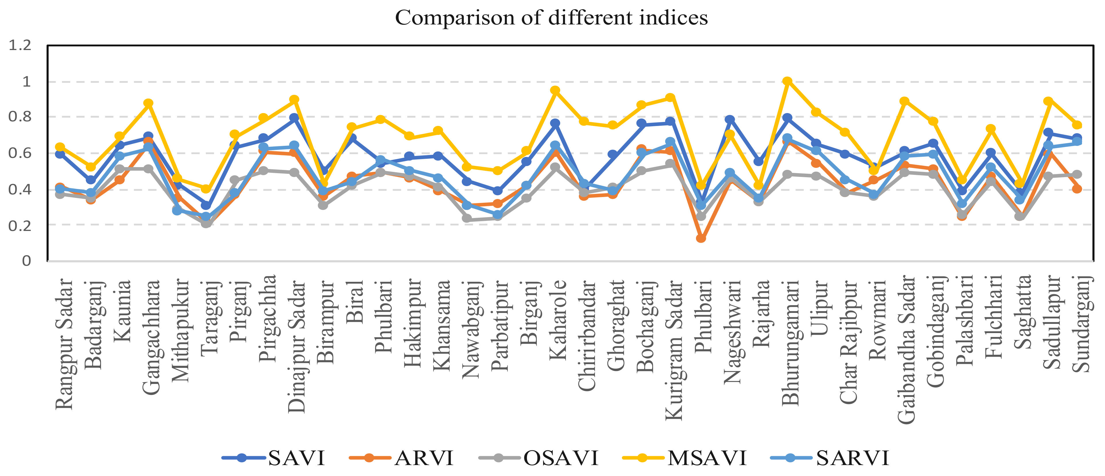
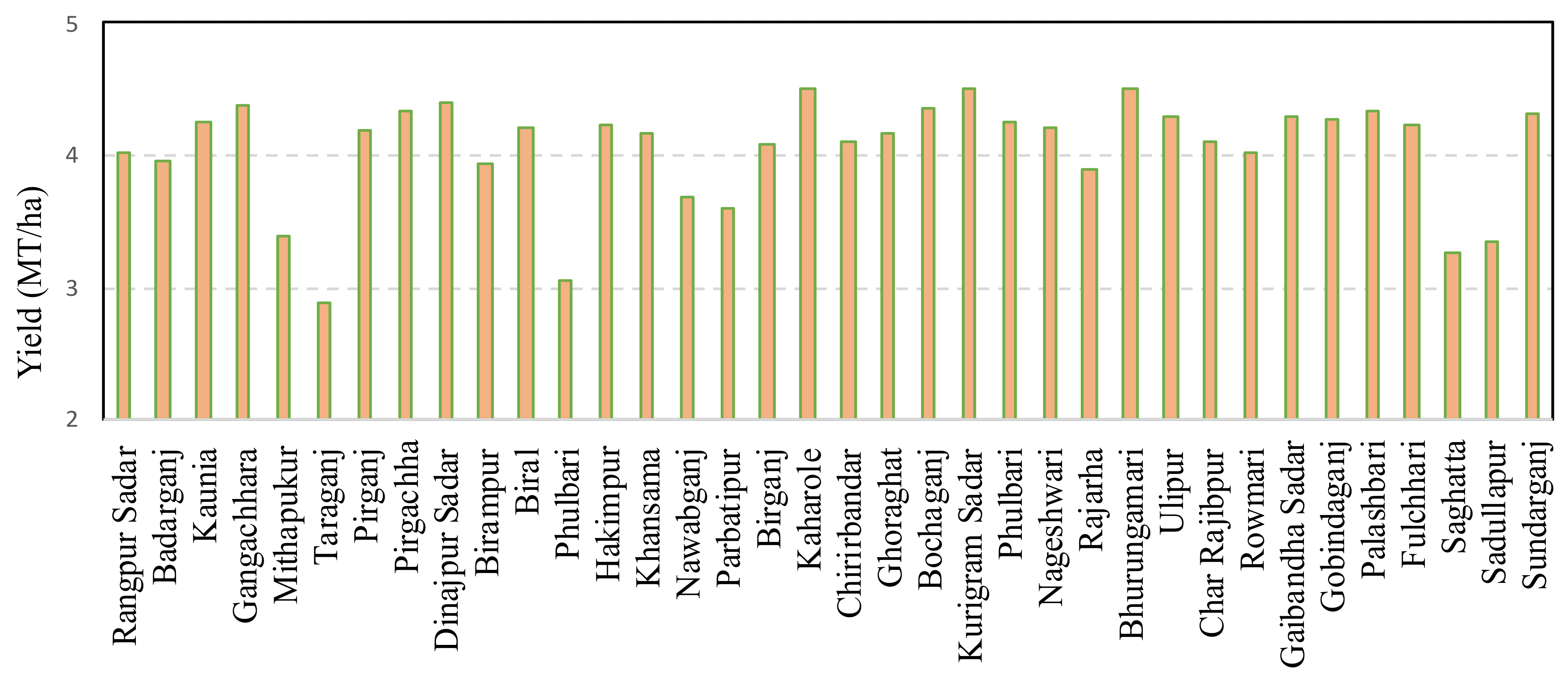
The detected fertile zone was verified by ground reference data. The time series datasets played a vital role in developing and validating the yield prediction models. In Bangladesh, nearly 80% of the total land is allocated solely to rice cultivation [62]. Additionally, in the northwestern part of the country, approximately 70% [63,64,65] of the land is cultivated with dry season irrigated rice (boro rice). To facilitate further analysis, the major rice crop was carefully chosen for approval. The suitable area was verified by ground truth yield data. The yield data of dry season irrigated rice were collected from the Department of Agricultural Extension (DAE), Ministry of Agriculture, Bangladesh, for the 36 subdistricts in 2017–2020 to evaluate the accuracy of the land suitability analysis (Figure 4 and Figure 5). After preparing the data in Microsoft Excel, the correlations among the five selected indices were evaluated.

2.8. Yield Prediction and Analysis

The performances of the yield prediction models were examined by field data. After the correlations among the five selected vegetation indices were established, the yield map was developed. Simple and multiple regression analyses were carried out between the mean values of the vegetation indices and the ground referenced data of the dry season irrigated rice to determine the best-fitted models for rice production. These data were classified to evaluate the production that occurred between 2017 and 2020. The SAVI, ARVI, SARVI, MSAVI, and OSAVI values were aggregated into a time series pattern (Appendix A). The yield data were compared through regression. The five vegetation index values were collected from reference points in the 36 subdistricts. Ground truth data information was obtained from the 36 subdistricts, and the yield was reported in metric tons per hector (MT/ha).

3. Results

3.1. Land Suitability Analysis

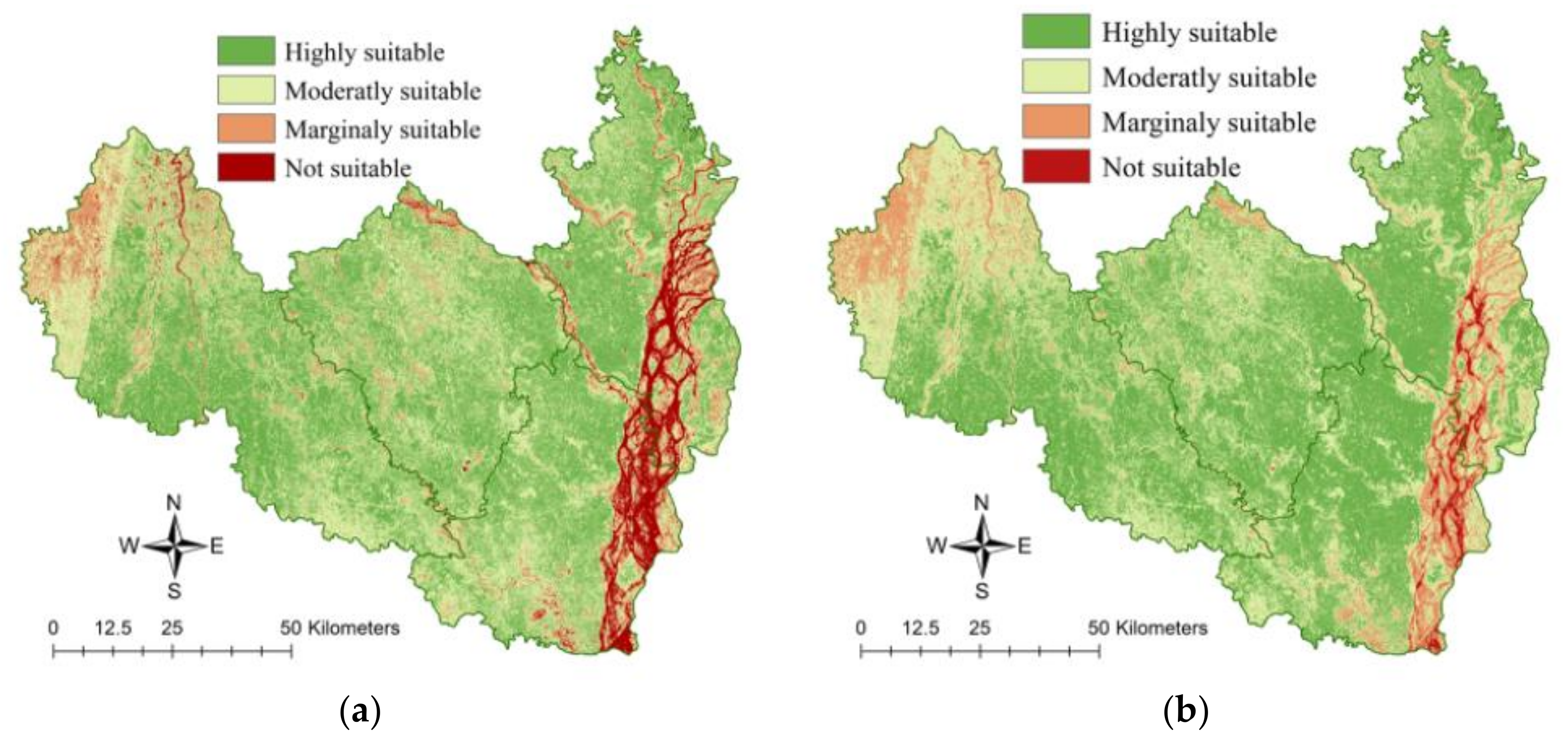
The weighted linear model was used to prioritize the weights of each criterion to generate the land suitability assessment. First, the variables were analyzed as equally weighted linear combinations. Second, the suitability assessment was carried out by a fuzzy membership function to verify the consistency of the two procedure results (Table 4). The land fertility analysis (Figure 6a) with equal weights showed that 43% of the land (1832 km2) was highly suitable, 41% of the land (1747 km2) was moderately suitable, and 10% of the land (426 km2) was marginally suitable. In addition, the restricted zone was defined as an unsuitable area. In this research, the unsuitable area was found to cover 6% (256 km2). However, the land suitability analysis using the fuzzy membership function (Figure 6b) showed that 48% (2045 km2) of the land area consisted of the most suitable area, 39% of the land (1661 km2) was moderately suitable, and 7% of the land (298 km2) was marginally suitable. In addition, restricted areas accounted for 6% of the land area. In fuzzy overlay analysis, 256 km2 of the area was classified as fallow land that is not suitable for cultivation.

3.2. Yield Estimation

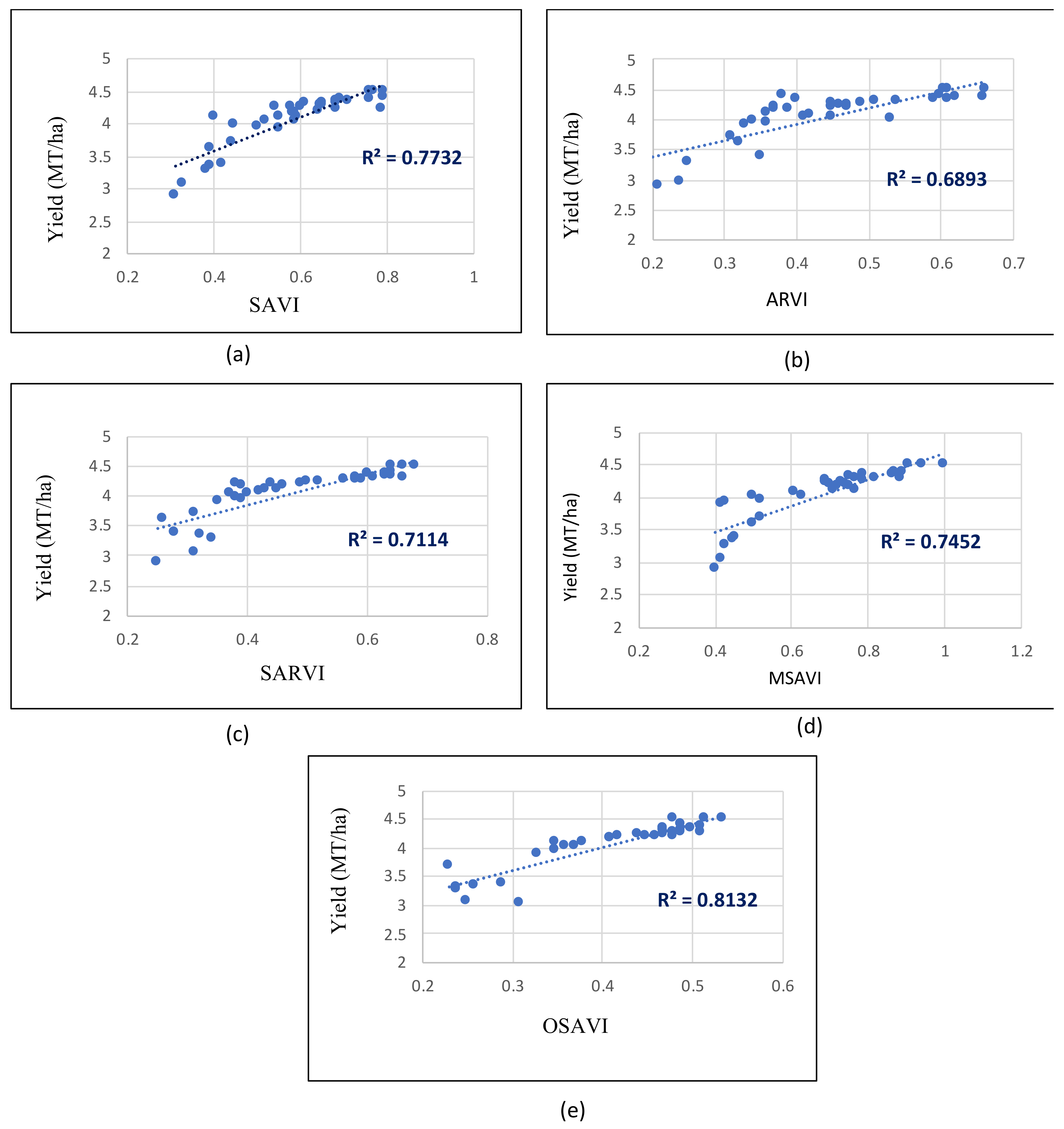
The predictors derived from the satellite imagery in the form of spectral bands or vegetation indices (SAVI, SAVI, ARVI, SARVI, MSAVI, and OSAVI) were the most effective spectral parameters for predicting rice yield (Figure 7). In addition, the individual index values were extracted from the ground truth information (Figure 4 and Figure 5) for the subdistricts that were located in the highly suitable areas. A trend line approach was used to verify the index influences at different study points (Figure 8). Regression analysis was performed between the vegetation indices and the observed yield. The SAVI, SARVI, ARVI, MSAVI, and OSAVI values were obtained from satellite imagery from 2017–2020 (Table 5). The results showed good accuracy in the regression analysis using SAVI (R2 = 77.3%), ARVI (R2 = 68.9%), SARVI (R2 = 71.1%), MSAVI (R2 = 74.5%) and OSAVI (R2 = 81.2%) (Figure 9). From the multiple regression model, it was observed that using more than one variable for the yield prediction increased the model accuracy by enhancing the R 2 value. However, the best-fitted models were obtained using the SAVI-ARVI-SARVI-MSAVI-OSAVI composite vegetation index. The yield prediction model with the composite index had a goodness of fit of R 2 = 0.839. The model was used to estimate the yield in the time series dataset (Table 6).
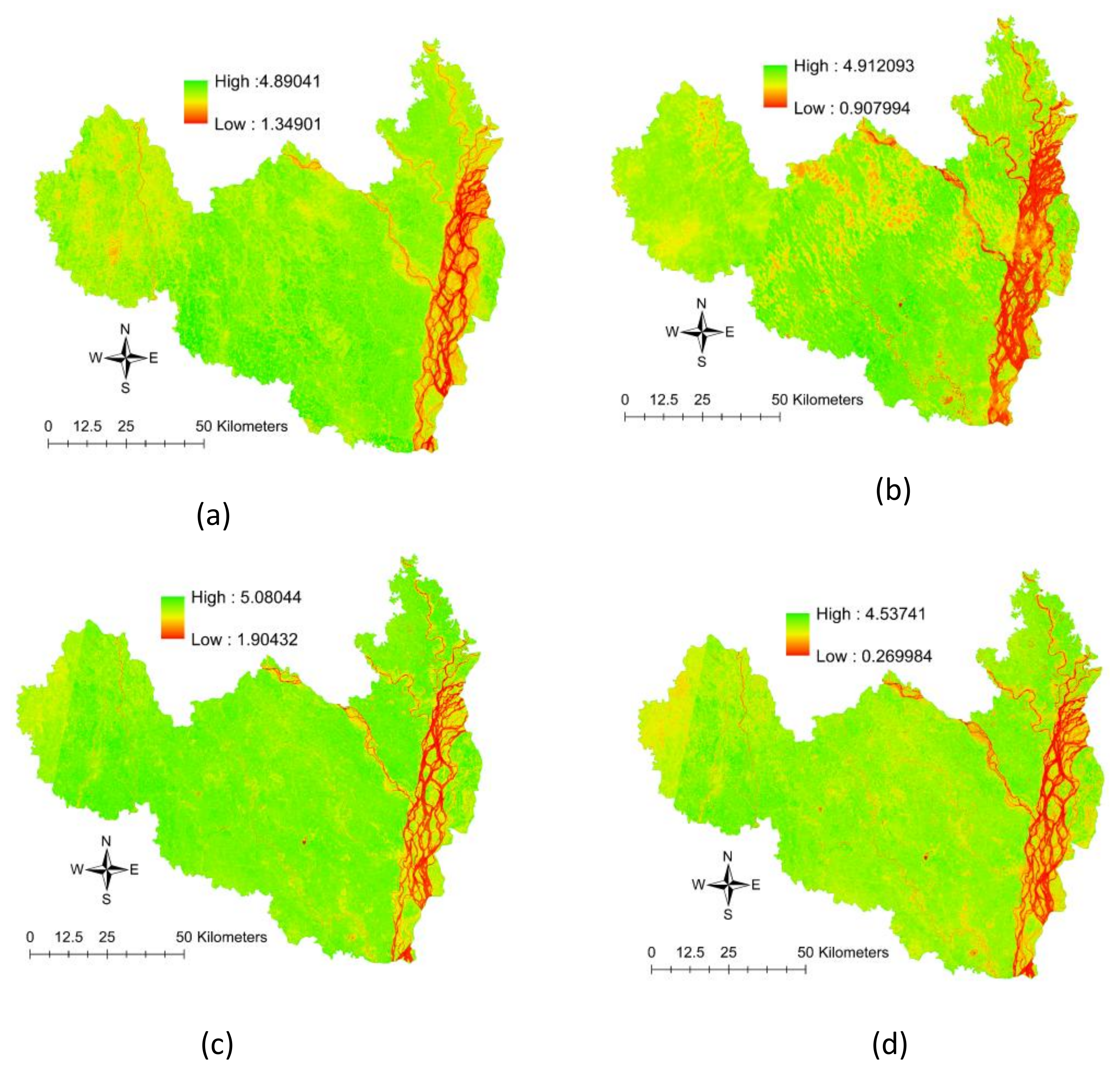
The developed yield map indicated that in 2017, the maximum yield was 4.59 MT/ha (Figure 10). Furthermore, in 2018 and in 2019, it was 4.9 MT/ha and 5.08 MT/ha, respectively. For 2020, the predicted yield range appeared to be between 0.269 MT/ha and 4.537 MT/ha.

4. Discussion

This research provided a comprehensive strategy to create agricultural land use plans for cultivation considering suitable conditions, which were derived from satellite remote sensing data. Previously, much of the research conducted only reported land suitability for site-specific plans or single-cropping plans [66,67]. However, this research attempted to develop an overall land suitability assessment using soil-vegetation representative variables that extracted only satellite remote sensing data from the GIS platform when field soil sampling is inconvenient and expensive. Applying only remote satellite datasets to assess suitable land conditions was a source of concern that added a new feature to MCDM-land suitability analyses. In this study, the reliability of five vegetation indices was verified by a regression analysis that incorporated ground truth yield data, and the results were used for yield map preparation. Vegetation phenology analyses have potential [11,14] in estimating yield prediction with good accuracy in highly suitable areas. In addition, two topological factors (slope and elevation) and another environmental parameter, land surface temperature, were extracted from the USGS, which ensured better performance of the results in land use planning.
Either the AHP-based weighted overlay or equal-overlay technique is typically applied in most studies [68,69,70]; few studies have conducted fuzzy membership methods employed in the GIS platform by incorporation with the AHP technique [69,71,72]. Some studies have conducted farmland assessments based on soil testing [73,74]; however, considering the preparation of a suitable map for agricultural land using soil-represented remote sensing data for the linear combination of the F-MCDM approach is a new dimension of this research. A multicriteria decision-making system was applied to reduce the biases in the analysis. Variation in the land surface temperature was an important factor in this area and influenced the locations considered most suitable for crop cultivation. Moreover, atmospherically restricted vegetation indices (ARVI) and soil adjusted atmospherically restricted vegetation indices (SARVI) were used to reduce the biases associated with atmospheric effects.
Most of the suitable lands were located in the northern part, and marginally suitable lands were mostly located in the northwestern part; this result was likely due to the influence of high elevation. In addition, unsuitable zones were found mostly in the eastern part due to the presence of water bodies that are not arable for cultivation along with other adverse edaphic factors. Previous studies had the limitation of obtaining inappropriate validation results due to inadequate ground reference information. In this research, the validation of the results was accomplished by physical verification with the corresponding time series yield data of the most cultivated crop, dry season irrigated rice, which usually grows over 70% [65] of the agricultural land area. The suitable conditions were not verified by the other crop yield data, which was the main limitation of this research.

5. Conclusions

This research established a method to identify the most suitable agricultural land by using the potentiality of satellite remote sensing data integrated with weighted linear combinations and fuzzy multicriteria analyses in a GIS platform. The multicriteria decision analysis was performed for suitability assessment using eight criteria: elevation, slope, and LST vegetation indices (SAVI, ARVI, SARVI, MSAVI, and OSAVI). To derive a more accurate result, a land use/land cover layer was also used to mask restricted zones. The land suitability analysis with equal weights showed that 43% of the land (1832 km2) was highly suitable, 41% of the land (1747 km2) was moderately suitable, and 10% of the land (426 km2) was marginally suitable. Conversely, expert knowledge was also considered, along with consistent assessments when using the fuzzy membership function; 48% of the land (2045 km2) was highly suitable, 39% of the land (2045 km2) was moderately suitable, and 7% of the land (298 km2) was marginally suitable. The yield estimation using SAVI (R2 = 77.3%), ARVI (R2 = 68.9%), SARVI (R2 = 71.1%), MSAVI (R2 = 74.5%), and OSAVI (R2 = 81.2%) showed a good accuracy. In addition, every combination of these five indices represented the best accuracy (R2 = 0.839), which was used to develop the yield maps for the corresponding years (2017–2020). The results of the land suitability evaluation for field crops will be very useful in the decision-making process to increase production as well as for the sustainable management of agricultural lands. Thus, the influence of vegetation index evaluations, suitable condition assessments, and yield prediction models is essential for understanding future land use and production trends in the agricultural crop sector in Bangladesh, as well as other applications.

Author Contributions

Research Investigation, Methodology, Data Curation, Analysis, Interpretation of Results, and Writing—Original Draft, R.B.M.; Resources and Editing, R.N.; Research Conceptualization, Editing, Review and Supervision T.A.; All authors have read and agreed to the published version of the manuscript.

Funding

This research received no external funding.

Institutional Review Board Statement

Not applicable.

Informed Consent Statement

Not applicable.

Data Availability Statement

The data used is primarily reflected in the article. Other relevant data is available from the authors upon request.

Acknowledgments

We would like to express their sincere gratitude to the Graduate School of Life and Environmental Sciences, the University of Tsukuba, for supporting this research in land fertility assessment and index evolution using satellite datasets. We are sincerely thankful to the United States Geological Survey (USGS) for providing Landsat 8 OLI and Shuttle Radar Topography Mission (SRTM) data free of cost. We are grateful to the Department of Agricultural Extension (DAE), Ministry of Agriculture, Bangladesh, for their cordial support by providing ground reference yield data for 36 subdistricts from 2017–2020. Furthermore, we are also thankful to the Japan International Research Center for Agricultural Sciences (JIRCAS) for technical support to pursue this research in Japan.

Conflicts of Interest

The authors declare no conflict of interest.

Appendix A

Table A1. SAVI, ARVI, SARVI, MSAVI and OSAVI from 2017–2020 for 36 subunits.
Ground PointsSAVIARVISARVIMASAVIOSAVI
20172018201920202017201820192020201720182019202020172018201920202017201820192020
10.5010.5570.6980.5930.3880.420.3980.430.3880.420.4180.3030.6880.5820.6680.6020.3880.4020.4580.401
20.4450.540.350.420.4050.3030.3550.320.3450.340.3850.320.5450.540.550.4520.4150.3940.4350.302
30.5340.650.710.690.4140.5250.5010.390.5440.4750.5310.490.6840.7850.7390.590.5440.5950.5910.589
40.6430.670.6820.770.690.660.710.570.5390.5060.510.470.8690.8660.9190.8270.690.660.610.57
50.4080.5190.4170.3750.420.350.290.3550.2820.2850.3090.26550.4420.4750.47290.39490.2920.2950.3290.195
60.3210.4010.3150.2270.2510.2010.2240.190.2210.210.2350.20.310.410.5010.40.6310.6210.68270.62
70.4720.5970.6980.7840.3940.3970.3850.3010.4480.4470.470.4210.6740.7070.7450.6810.3640.3970.3770.5501
80.5950.6710.7720.6890.6810.6610.50.590.48010.510.540.4390.79810.79810.8290.7390.6810.610.50.79
90.7990.7970.7790.7690.6690.5770.670.5390.4790.5080.5290.4490.7990.8960.990.8590.3790.3860.490.289
100.4790.6210.6310.3030.330.3660.4310.310.330.320.310.3030.4150.4360.48310.4230.50.4360.4310.383
110.7480.6990.6920.5980.480.4870.490.440.480.390.420.4040.680.7470.8420.7240.6080.5470.6420.474
120.5840.3940.7330.43870.540.490.5390.3870.4540.490.490.4870.7540.7490.890.7070.540.490.490.487
130.5190.6030.6450.5380.4790.460.470.4390.4790.460.5070.450.6790.6860.7470.6690.4790.460.4970.4069
140.6880.7890.6670.5820.380.4390.410.3120.4080.4150.4780.370.7180.7390.7410.7020.3580.3090.3710.252
150.4840.4110.5830.2920.3120.3010.3910.2820.220.2910.230.2120.440.310.6230.520.240.310.330.182
160.4190.3720.440.360.350.3120.340.300.290.220.2540.220.390.320.240.50.390.4320.4240.405
170.450.5620.6850.5410.430.5020.4250.3410.350.3730.3850.310.6550.6420.6350.56010.6450.6220.7350.621
180.7860.6990.7940.7440.6760.6040.61440.5440.560.5040.51440.49440.9760.9040.9910.9040.4760.4040.47440.384
190.4010.360.5480.2970.40.360.380.3070.3490.3950.4180.32790.740.7360.8580.770.340.4260.4340.377
200.4870.6010.7510.4750.3870.3970.4410.250.4870.370.4310.3750.7870.7970.7940.6950.5870.6070.6410.595
210.7880.6920.7890.7740.6960.6520.660.5010.5310.5020.530.4640.7610.8620.850.8240.6610.6920.6950.584
220.7870.7930.80130.6990.6170.7710.5350.5050.5070.560.5750.5050.9770.91610.85350.9050.3370.3010.3350.29
230.40270.2120.450.2220.1270.1020.1650.1020.22770.2620.2750.2220.43770.4320.4250.3820.4770.4620.54950.442
240.7950.8060.7990.7080.4150.450.5060.4270.4850.450.4760.440.67250.650.8160.6970.3850.3850.3460.27
250.650.3930.6930.4920.350.3430.330.3020.3250.330.3730.3020.350.5330.4930.3420.550.7330.7830.642
260.790.7620.8180.7990.690.6620.680.5980.4790.4690.4980.49980.9790.96620.9980.9980.6090.6220.6480.591
270.750.540.770.550.450.540.670.520.4750.4880.4790.40220.7950.8540.8470.7820.4650.4540.4970.382
280.6930.4870.6880.4910.390.4180.4180.2810.390.4080.4080.3210.7090.7180.7380.7010.390.3980.3980.2971
290.5120.6050.5860.360.4910.4250.560.350.320.350.360.3950.450.520.6030.4950.520.550.660.5
300.7010.5030.6290.6350.510.5230.6190.4850.4970.4530.5090.47850.7610.8530.8490.7850.610.530.6490.585
310.6220.7310.6870.5470.5120.5010.5910.470.4920.5010.4890.4370.76520.7510.8480.6970.5520.5910.6480.547
320.3390.440.4860.2950.270.2240.2560.2350.2490.2470.2990.2250.4390.4740.4860.3850.370.3240.3260.295
330.5680.6470.7040.5030.480.470.490.430.460.440.440.430.60.7470.8440.730.560.470.6440.43
340.3920.450.440.230.280.2350.3140.1930.280.2050.2940.2130.4380.4450.4240.4030.320.350.3240.33
350.7910.590.7870.6860.570.590.6070.5860.4710.5930.4570.3890.8710.8590.9470.7860.510.790.67470.586
360.5980.6970.7780.6090.380.4030.4580.3950.4880.4470.5490.4350.6880.5820.6680.6020.680.6940.69480.575

References

  1. Kennedy, C.M.; Hawthorne, P.L.; Miteva, D.A.; Baumgarten, L.; Sochi, K.; Matsumoto, M.; Evans, J.S.; Polasky, S.; Hamel, P.; Vieira, E.M.; et al. Optimizing land use decision-making to sustain Brazilian agricultural profits, biodiversity and ecosystem services. Biol. Conserv. 2016, 204, 221–230. [Google Scholar] [CrossRef] [Green Version]
  2. Pimentel, D.; Burgess, M. Soil Erosion Threatens Food Production. Agriculture 2013, 3, 443–463. [Google Scholar] [CrossRef] [Green Version]
  3. Jyoti, N.A.; Lal, R.; Das, A.K. Ethnopedology and soil quality of bamboo (Bambusa sp.) based agroforestry system. Sci. Total. Environ. 2015, 521, 372–379. [Google Scholar] [CrossRef]
  4. Niemeijer, D.; Mazzucato, V. Moving beyond indigenous soil taxonomies: Local theories of soils for sustainable development. Geoderma 2003, 111, 403–424. [Google Scholar] [CrossRef]
  5. Mazza, A.; Gargiulo, M.; Scarpa, G.; Gaetano, R. Estimating the NDVI from SAR by Convolutional Neural Networks. In Proceedings of the IGARSS 2018 IEEE International Geoscience and Remote Sensing Symposium, Valencia, Spain, 22–27 July 2018; IEEE: New York, NY, USA, 2018; pp. 1954–1957. [Google Scholar]
  6. Li, Y.; Chen, W.; Zhang, Y.; Tao, C.; Xiao, R.; Tan, Y. Accurate cloud detection in high-resolution remote sensing imagery by weakly supervised deep learning. Remote. Sens. Environ. 2020, 250, 112045. [Google Scholar] [CrossRef]
  7. Ennouri, K.; Kallel, A. Remote Sensing: An Advanced Technique for Crop Condition Assessment. Math. Probl. Eng. 2019, 2019, 1–8. [Google Scholar] [CrossRef] [Green Version]
  8. Olivero, J.; Real, R.; Márquez, A.L. Fuzzy Chorotypes as a Conceptual Tool to Improve Insight into Biogeographic Patterns. Syst. Biol. 2011, 60, 645–660. [Google Scholar] [CrossRef] [Green Version]
  9. Elsheikh, R.; Shariff, A.R.B.M.; Amiri, F.; Ahmad, N.B.; Balasundram, S.K.; Soom, M.A.M. Agriculture Land Suitability Evaluator (ALSE): A decision and planning support tool for tropical and subtropical crops. Comput. Electron. Agric. 2013, 93, 98–110. [Google Scholar] [CrossRef] [Green Version]
  10. Kazemi, H.; Akinci, H. A land use suitability model for rainfed farming by Multi-criteria Decision-making Analysis (MCDA) and Geographic Information System (GIS). Ecol. Eng. 2018, 116, 1–6. [Google Scholar] [CrossRef]
  11. Habibie, M.I.; Noguchi, R.; Shusuke, M.; Ahamed, T. Land suitability analysis for maize production in Indonesia using satellite remote sensing and GIS-based multicriteria decision support system. GeoJournal 2019, 1–31. [Google Scholar] [CrossRef]
  12. Food and Agriculture Organization. A Framework for Land Evaluation; Food and Agriculture Organization: Rome, Italy, 1976. [Google Scholar]
  13. Tucker, C.J. Red and photographic infrared linear combinations for monitoring vegetation. Remote Sens. Environ. 1979, 8, 127–150. [Google Scholar] [CrossRef] [Green Version]
  14. Das, A.C.; Noguchi, R.; Ahamed, T. Integrating an Expert System, GIS, and Satellite Remote Sensing to Evaluate Land Suitability for Sustainable Tea Production in Bangladesh. Remote Sens. 2020, 12, 4136. [Google Scholar] [CrossRef]
  15. Romano, G.; Sasso, P.D.; Liuzzi, G.T.; Gentile, F. Multi-criteria decision analysis for land suitability mapping in a rural area of Southern Italy. Land Use Policy 2015, 48, 131–143. [Google Scholar] [CrossRef]
  16. Campos, I.; González-Gómez, L.; Villodre, J.; González-Piqueras, J.; Suyker, A.E.; Calera, A. Remote sensing-based crop biomass with water or light-driven crop growth models in wheat commercial fields. Field Crop. Res. 2018, 216, 175–188. [Google Scholar] [CrossRef]
  17. Essougong, U.P.K.; Slingerland, M.; Mathé, S.; Vanhove, W.; Ngome, P.I.T.; Boudes, P.; Giller, K.E.; Woittiez, L.S.; Leeuwis, C. Farmers’ Perceptions as a Driver of Agricultural Practices: Understanding Soil Fertility Management Practices in Cocoa Agroforestry Systems in Cameroon. Hum. Ecol. 2020, 48, 709–720. [Google Scholar] [CrossRef]
  18. Bangladesh Bureau of Statistics (BBS). Statistics and Informatics Division (SID) Ministry of Planning: Population and Housing Census 2011; Bangladesh Bureau of Statistics: Dacca, Bangladesh, 2011. [Google Scholar]
  19. Bangladesh Bureau of Statistics (BBS). Statistical Pocket Book Bangladesh 2016; Ministry of Planning: Dhaka, Bangladesh, 2018. [Google Scholar]
  20. Bozdağ, A.; Yavuz, F.; Günay, A.S. AHP and GIS based land suitability analysis for Cihanbeyli (Turkey) County. Environ. Earth Sci. 2016, 75, 813. [Google Scholar] [CrossRef]
  21. Senanayake, S.; Pradhan, B.; Huete, A.; Brennan, J. Assessing Soil Erosion Hazards Using Land-Use Change and Landslide Frequency Ratio Method: A Case Study of Sabaragamuwa Province, Sri Lanka. Remote Sens. 2020, 12, 1483. [Google Scholar] [CrossRef]
  22. Ashford, S.A.; Sitar, N.; Lysmer, J.; Deng, N. Topographic effects on the seismic response of steep slopes. Bull. Seismol. Soc. Am. 1997, 87, 701–709. [Google Scholar]
  23. El Kateb, H.; Zhang, H.; Zhang, P.; Mosandl, R. Soil erosion and surface runoff on different vegetation covers and slope gradients: A field experiment in Southern Shaanxi Province, China. Catena 2013, 105, 1–10. [Google Scholar] [CrossRef]
  24. Zolekar, R.B.; Bhagat, V.S. Multi-criteria land suitability analysis for agriculture in hilly zone: Remote sensing and GIS approach. Comput. Electron. Agric. 2015, 118, 300–321. [Google Scholar] [CrossRef]
  25. Koulouri, M.; Giourga, C. Land abandonment and slope gradient as key factors of soil erosion in Mediterranean terraced lands. Catena 2007, 69, 274–281. [Google Scholar] [CrossRef]
  26. Nahusenay, A.; Kibebew, K. Land suitability evaluation in Wadla Delanta Massif of north central highlands of Ethiopia for rainfed crop production. Afr. J. Agric. Res. 2015, 10, 1595–1611. [Google Scholar] [CrossRef] [Green Version]
  27. Novara, A.; Gristina, L.; Sala, G.; Galati, A.; Crescimanno, M.; Cerdà, A.; Badalamenti, E.; La Mantia, T. Agricultural land abandonment in Mediterranean environment provides ecosystem services via soil carbon sequestration. Sci. Total Environ. 2017, 576, 420–429. [Google Scholar] [CrossRef] [Green Version]
  28. Basche, A.D.; Archontoulis, S.V.; Kaspar, T.C.; Jaynes, D.B.; Parkin, T.B.; Miguez, F.E. Simulating long-term impacts of cover crops and climate change on crop production and environmental outcomes in the Midwestern United States. Agric. Ecosyst. Environ. 2016, 218, 95–106. [Google Scholar] [CrossRef] [Green Version]
  29. Jeevalakshmi, D.; Narayana Reddy, S.; Manikiam, B. Land surface temperature retrieval from LANDSAT data using emissivity estimation. Int. J. Appl. Eng. Res. 2017, 12, 9679–9687. Available online: https://www.ripublication.com/ijaer17/ijaerv12n20_57.pdf (accessed on 1 January 2021).
  30. De Jesus, J.B.; Santana, I.D.M. Estimation of land surface temperature in caatinga area using Landsat 8 data. J. Hyperspectral Remote Sens. 2017, 7, 150–157. Available online: https://periodicos.ufpe.br/revistas/jhrs/article/viewFile/22766/pdf (accessed on 1 January 2021).
  31. Jiang, Z.; Huete, A.R.; Chen, J.; Chen, Y.; Li, J.; Yan, G.; Zhang, X. Analysis of NDVI and scaled difference vegetation index retrievals of vegetation fraction. Remote Sens. Environ. 2006, 101, 366–378. [Google Scholar] [CrossRef]
  32. Huete, A. A soil-adjusted vegetation index (SAVI). Remote Sens. Environ. 1988, 25, 295–309. [Google Scholar] [CrossRef]
  33. Somvanshi, S.S.; Kumari, M. Comparative analysis of different vegetation indices with respect to atmospheric particulate pollution using sentinel data. Appl. Comput. Geosci. 2020, 7, 100032. [Google Scholar] [CrossRef]
  34. Kaufman, Y.J.; Tanre, D. Atmospherically resistant vegetation index (ARVI) for EOS-MODIS. IEEE Trans. Geosci. Remote Sens. 1992, 30, 261–270. [Google Scholar] [CrossRef]
  35. Haboudane, D.; Miller, J.R.; Pattey, E.; Zarco-Tejada, P.J.; Strachan, I.B. Hyperspectral vegetation indices and novel algorithms for predicting green LAI of crop canopies: Modeling and validation in the context of precision agriculture. Remote Sens. Environ. 2004, 90, 337–352. [Google Scholar] [CrossRef]
  36. Kim, M.S.; Daughtry, C.S.T.; Chappelle, E.W.; McMurtrey, J.E.; Walthall, C.L. The Use of High Spectral Resolution Bands for Estimating Absorbed Photosynthetically Active Radiation. In Proceedings of the 6th Symposium on Physical Measurements and Signatures in Remote Sensing, Val D’Isere, France, 17–21 January 1994; pp. 299–306. [Google Scholar]
  37. Richardson, A.J.; Wiegand, C.L. Distinguishing vegetation from soil background information. Photogramm. Eng. Remote Sens. 1977, 43, 1541–1552. [Google Scholar]
  38. Mao, Z.-H.; Deng, L.; Duan, F.-Z.; Li, X.-J.; Qiao, D.-Y. Angle effects of vegetation indices and the influence on prediction of SPAD values in soybean and maize. Int. J. Appl. Earth Obs. Geoinf. 2020, 93, 102198. [Google Scholar] [CrossRef]
  39. Mwinuka, P.R.; Mbilinyi, B.P.; Mbungu, W.B.; Mourice, S.K.; Mahoo, H.; Schmitter, P. The feasibility of hand-held thermal and UAV-based multispectral imaging for canopy water status assessment and yield prediction of irrigated African eggplant (Solanum aethopicum L). Agric. Water Manag. 2021, 245, 106584. [Google Scholar] [CrossRef]
  40. Zadeh, L.A. Fuzzy sets. Inf. Control. 1965, 8, 338–353. [Google Scholar] [CrossRef] [Green Version]
  41. Bellman, R.E.; Zadeh, L.A. Decision-Making in a Fuzzy Environment. Manag. Sci. 1970, 17, 141. [Google Scholar] [CrossRef]
  42. Mitchell, S.; Cohen, K. Fuzzy Logic Decision Making for Autonomous Robotic Applications. In Proceedings of the 2014 IEEE 6th International Conference on Awareness Science and Technology (iCAST), Paris, France, 29–31 October 2014; IEEE: New York, NY, USA, 2014; pp. 1–6. [Google Scholar]
  43. Gitari, H.I.; Gachene, C.K.K.; Karanja, N.N.; Kamau, S.; Nyawade, S.; Schulte-Geldermann, E. Potato-legume intercropping on a sloping terrain and its effects on soil physico-chemical properties. Plant Soil 2019, 438, 447–460. [Google Scholar] [CrossRef]
  44. Shimoda, S.; Kanno, H.; Hirota, T. Time series analysis of temperature and rainfall-based weather aggregation reveals significant correlations between climate turning points and potato (Solanum tuberosum L) yield trends in Japan. Agric. For. Meteorol. 2018, 263, 147–155. [Google Scholar] [CrossRef]
  45. GRiSP. Rice Almanac, 4th ed.; Global Rice Science Partnership: Los Baños, Philippines, 2013. [Google Scholar]
  46. Yalew, S.G.; Van Griensven, A.; Mul, M.L.; Van Der Zaag, P. Land suitability analysis for agriculture in the Abbay basin using remote sensing, GIS and AHP techniques. Model. Earth Syst. Environ. 2016, 2, 1–14. [Google Scholar] [CrossRef] [Green Version]
  47. Ceglar, A.; Toreti, A.; Prodhomme, C.; Zampieri, M.; Turco, M.; Doblas-Reyes, F.J. Land-surface initialisation improves seasonal climate prediction skill for maize yield forecast. Sci. Rep. 2018, 8, 1–9. [Google Scholar] [CrossRef] [Green Version]
  48. Samanta, S.; Pal, B.; Pal, D.K. Land Suitability Analysis for Rice Cultivation Based on Multi-Criteria Decision Approach through GIS. Data Base. Int. J. Sci. and Emerg. Technol. 2011, 2, 12–20. [Google Scholar]
  49. Ren, H.; Feng, G. Are soil-adjusted vegetation indices better than soil-unadjusted vegetation indices for above-ground green biomass estimation in arid and semi-arid grasslands? Grass Forage Sci. 2014, 70, 611–619. [Google Scholar] [CrossRef]
  50. Venancio, L.P.; Mantovani, E.C.; Amaral, C.H.D.; Neale, C.M.U.; Gonçalves, I.Z.; Filgueiras, R.; Campos, I. Forecasting corn yield at the farm level in Brazil based on the FAO-66 approach and soil-adjusted vegetation index (SAVI). Agric. Water Manag. 2019, 225, 105779. [Google Scholar] [CrossRef]
  51. Sonobe, R.; Yamaya, Y.; Tani, H.; Wang, X.; Kobayashi, N.; Mochizuki, K.-I. Crop classification from Sentinel-2-derived vegetation indices using ensemble learning. J. Appl. Remote Sens. 2018, 12, 026019. [Google Scholar] [CrossRef] [Green Version]
  52. Svinurai, W.; Hassen, A.; Tesfamariam, E.; Ramoelo, A. Performance of ratio-based, soil-adjusted and atmospherically corrected multispectral vegetation indices in predicting herbaceous aboveground biomass in a Colophospermum mopane tree-shrub savanna. Grass Forage Sci. 2018, 73, 727–739. [Google Scholar] [CrossRef]
  53. Cho, M.A.; Skidmore, A.K. Hyperspectral predictors for monitoring biomass production in Mediterranean mountain grasslands: Majella National Park, Italy. Int. J. Remote Sens. 2008, 30, 499–515. [Google Scholar] [CrossRef]
  54. Ren, H.; Zhou, G.; Zhang, F. Using negative soil adjustment factor in soil-adjusted vegetation index (SAVI) for aboveground living biomass estimation in arid grasslands. Remote Sens. Environ. 2018, 209, 439–445. [Google Scholar] [CrossRef]
  55. Gilabert, M.; González-Piqueras, J.; García-Haro, F.; Meliá, J. A generalized soil-adjusted vegetation index. Remote Sens. Environ. 2002, 82, 303–310. [Google Scholar] [CrossRef]
  56. Ayehu, G.T.; Besufekad, S.A. Land suitability analysis for rice production: A GIS based multi-criteria decision ap-proach. Am. J. Geogr. Inf. Syst. 2015, 4, 95–104. [Google Scholar] [CrossRef]
  57. Gerpacio, R.V.; Pingali, P.L. Tropical and Subtropical Maize in Asia: Production Systems, Constraints, and Research Priorities; CIMMYT: Texcoco, Mexico, 2007. [Google Scholar]
  58. Kihoro, J.; Bosco, N.J.; Murage, H. Suitability analysis for rice growing sites using a multicriteria evaluation and GIS approach in great Mwea region, Kenya. SpringerPlus 2013, 2, 265. [Google Scholar] [CrossRef] [Green Version]
  59. Purnamasari, R.A.; Noguchi, R.; Ahamed, T. Land suitability assessments for yield prediction of cassava using geospatial fuzzy expert systems and remote sensing. Comput. Electron. Agric. 2019, 166, 105018. [Google Scholar] [CrossRef]
  60. Fern, R.R.; Foxley, E.A.; Bruno, A.; Morrison, M.L. Suitability of NDVI and OSAVI as estimators of green biomass and coverage in a semi-arid rangeland. Ecol. Indic. 2018, 94, 16–21. [Google Scholar] [CrossRef]
  61. Bahrani, S.; Ebadi, T.; Ehsani, H.; Yousefi, H.; Maknoon, R. Modeling landfill site selection by multi-criteria decision making and fuzzy functions in GIS, case study: Shabestar, Iran. Environ. Earth Sci. 2016, 75, 1–14. [Google Scholar] [CrossRef]
  62. Mottaleb, K.A.; Kruseman, G.; Erenstein, O. Determinants of maize cultivation in a land-scarce rice-based economy: The case of Bangladesh. J. Crop. Improv. 2018, 32, 453–476. [Google Scholar] [CrossRef]
  63. Acharjee, T.K.; Van Halsema, G.; Ludwig, F.; Hellegers, P. Declining trends of water requirements of dry season Boro rice in the north-west Bangladesh. Agric. Water Manag. 2017, 180, 148–159. [Google Scholar] [CrossRef]
  64. Alamgir, S.; Furuya, J.; Kobayashi, S.; Mostafiz, R.B.; Ahmed, R. Farm income, inequality, and poverty among farm families of a flood-prone area in Bangladesh: Climate change vulnerability assessment. GeoJournal 2020, 1–25. [Google Scholar] [CrossRef]
  65. Zinat, M.R.M.; Salam, R.; Badhan, M.A.; Islam, A.R.M.T. Appraising drought hazard during Boro rice growing period in western Bangladesh. Int. J. Biometeorol. 2020, 64, 1687–1697. [Google Scholar] [CrossRef]
  66. Noorollahi, E.; Fadai, D.; Shirazi, M.A.; Ghodsipour, S.H. Land Suitability Analysis for Solar Farms Exploitation Using GIS and Fuzzy Analytic Hierarchy Process (FAHP)—A Case Study of Iran. Energies 2016, 9, 643. [Google Scholar] [CrossRef] [Green Version]
  67. Sulaiman, A.A.; Sulaeman, Y.; Mustikasari, N.; Nursyamsi, D.; Syakir, A.M. Increasing Sugar Production in Indonesia Through Land Suitability Analysis and Sugar Mill Restructuring. Land 2019, 8, 61. [Google Scholar] [CrossRef] [Green Version]
  68. Seyedmohammadi, J.; Sarmadian, F.; Jafarzadeh, A.A.; McDowell, R.W. Development of a model using matter element, AHP and GIS techniques to assess the suitability of land for agriculture. Geoderma 2019, 352, 80–95. [Google Scholar] [CrossRef]
  69. Pilevar, A.R.; Matinfar, H.R.; Sohrabi, A.; Sarmadian, F. Integrated fuzzy, AHP and GIS techniques for land suitability assessment in semi-arid regions for wheat and maize farming. Ecol. Indic. 2020, 110, 105887. [Google Scholar] [CrossRef]
  70. Tashayo, B.; Honarbakhsh, A.; Akbari, M.; Eftekhari, M. Land suitability assessment for maize farming using a GIS-AHP method for a semi-arid region, Iran. J. Saudi Soc. Agric. Sci. 2020, 19, 332–338. [Google Scholar] [CrossRef]
  71. Radočaj, D.; Jurišić, M.; Gašparović, M.; Plaščak, I. Optimal Soybean (Glycine max L.) Land Suitability Using GIS-Based Multicriteria Analysis and Sentinel-2 Multitemporal Images. Remote Sens. 2020, 12, 1463. [Google Scholar] [CrossRef]
  72. Amin, S.R.; Zhang, J.; Yang, M. Effects of Climate Change on the Yield and Cropping Area of Major Food Crops: A Case of Bangladesh. Sustainability 2015, 7, 898–915. [Google Scholar] [CrossRef] [Green Version]
  73. De Lima, T.M.; Weindorf, D.C.; Curi, N.; Guilherme, L.R.; Lana, R.M.; Ribeiro, B.T. Elemental analysis of Cerrado agricultural soils via portable X-ray fluorescence spectrometry: Inferences for soil fertility assessment. Geoderma 2019, 353, 264–272. [Google Scholar] [CrossRef]
  74. Buthelezi, N.N.; Hughes, J.C.; Modi, A. The use of scientific and indigenous knowledge in agricultural land evaluation and soil fertility studies of two villages in KwaZulu-Natal, South Africa. Afr. J. Agric. Res. 2013, 8, 507–518. [Google Scholar]
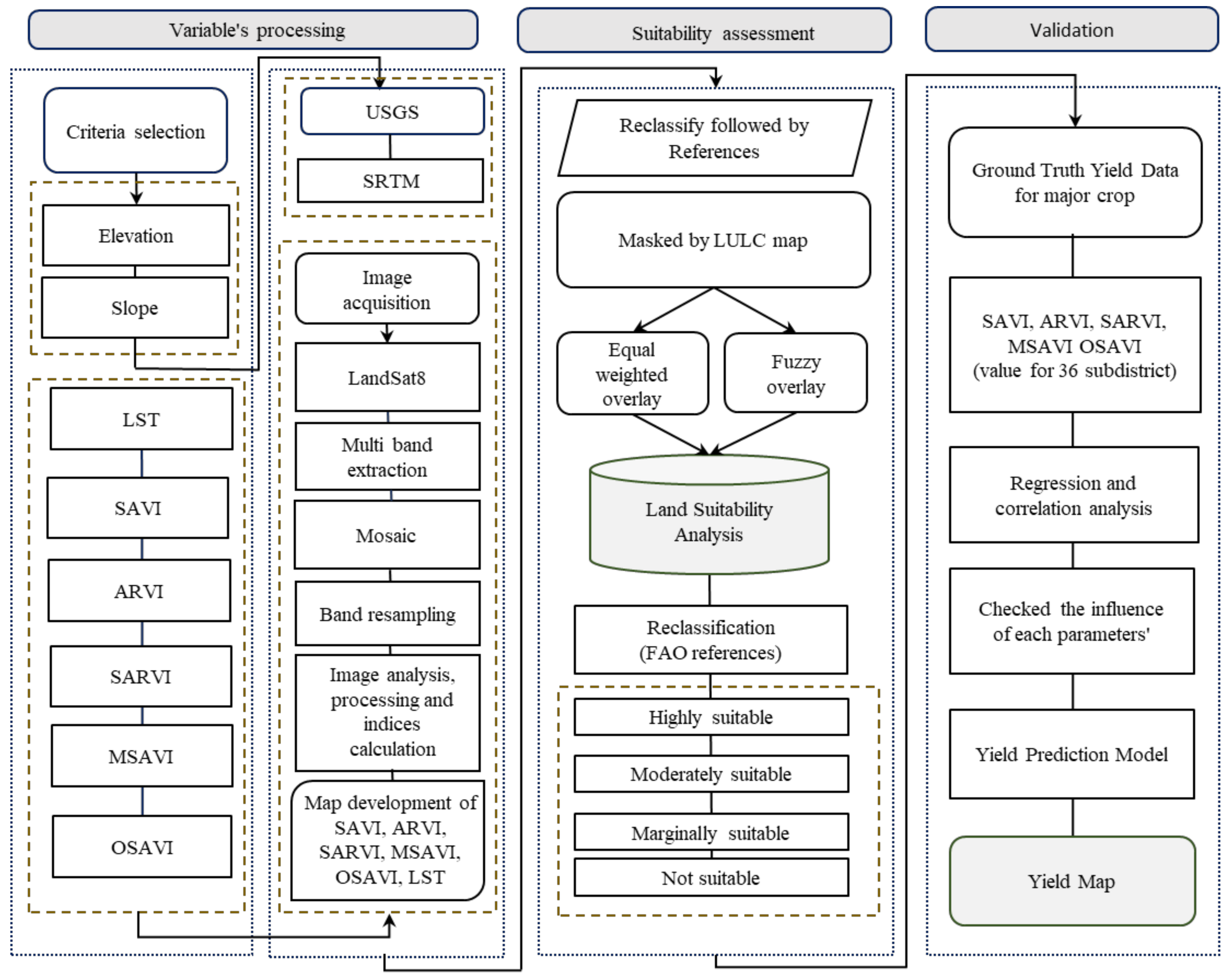
Figure 1. Framework for land suitability assessment using satellite remote sensing derived soil-vegetation indices.
Land 10 00223 g001
Figure 2. Study area: northern part of Bangladesh, four districts: Dinajpur, Rangpur, Gaibandha, and Kurigram.
Land 10 00223 g002
Figure 3. Criteria: (a) Elevation, (b) Slope, (c) LST, (d) SAVI, (e) ARVI, (f) SARVI, (g) MSAVI (h) OSAVI.
Land 10 00223 g003
Figure 4. Ground Reference information points in 36 subunits.
Land 10 00223 g004
Figure 5. Comparison of different indices and ground reference information points in 36 sub-units.
Land 10 00223 g005
Figure 6. Suitable classes of land suitability analysis using soil specified remote sensing data. (a) Equal weighted overlay. (b) Fuzzy overlay.
Land 10 00223 g006
Figure 7. Comparison of actual yield and predicted yield for different indices (a) SAVI (b)ARVI, (c) SARVI, (d) OSAVI, (e) MSAVI.
Land 10 00223 g007
Figure 8. Ground reference rice yield distributions in the 36 subunits.
Land 10 00223 g008
Figure 9. Regression analysis for vegetation indices and ground reference time series yield information. (a) SAVI, (b) ARVI, (c) SARVI, (d) OSAVI, (e) MSAVI.
Land 10 00223 g009
Figure 10. Yield prediction map (MT/ha) (a) 2017, (b) 2018, (c) 2019, (d) 2020.
Land 10 00223 g010
Table 1. List of data and original data sources for land suitability analysis.
NoDataNative FormatDescriptionSource
1Land Use Map92 small vector
blocks (point, line, polygon, and tabular)
Scale at 1:25,000m2019, SoB,
Bangladesh
2Elevation MaprasterExtracted from 3 m resolution2020, STRM
3Slope MaprasterDerived from 30-mresolution2020, STRM
4Land Surface Temperature (LST)rasterDerived from 30-m resolution2020, Landsat 8
5SAVI MaprasterDerived from 30-m resolution2020, Landsat 8, USGS
6ARVI MaprasterDerived from 30-m resolution2020, Landsat 8, USGS
7SARVI MaprasterDerived from 30-m resolution2020, Landsat 8, USGS
8MSAVI MaprasterDerived from 30-m resolution2020, Landsat 8, USGS
9OSAVI MaprasterDerived from 30-m resolution2020, Landsat 8, USGS
Table 2. Criteria reclassification for weighted linear combination.
CriteriaSuitability ClassSub CriteriaReference
S10–8%[24,40,41]
SlopeS28–15%
S315–25%
N>25%
S10–25[20,42,43]
ElevationS225–125
S3125–250
N>250
S120–25[29,44,45]
LSTS218–20
S315–18
N9–15, >25
S10.372483–0.797756[32,46,47]
SAVIS20.217838–0.372483
S30–0.217838
N−0.301941–0
ARVIS10.293275–0.885854[33,34,48]
S20.1542–0.293275
S30–0.1542
N−0.662108–0
S10.301197–0.671395[34,49,50]
SARVIS20.301197–0.16658
S30.16658–0
N−0.39713–0
S10.752112–1[37,46,51]
MSAVIS20.752112–0.443157
S30.443157–0
N−1–0
S10.245221–0.526082[38,46,52]
OSAVIS20.145221–0.248311
S30–0.145221
N−0.201272–0
Table 3. Criteria reclassification for Fuzzy membership function.
CriteriaMost Suitable ConditionMaximum Expectable ConditionMinimum Acceptable ConditionNot Fuzzy Member ReferenceFuzzy Membership Function
Slope<4°20°<20[43,56]F small
Elevation00–25250>250[20,57]F Gaussian
LST10 °C–20 °Cup to 35 °C10 °C>35 °C or <20 °C[45,58]F Gaussian
SAVI0.7978+1−1−0.3019 < SAVI < 0.7978[11,47,59]F Linear
ARVI0.8859+1−1−0.3971 < ARVI < 0.8859[33,34,48]F Linear
SARVI0.6713+1−1−0.3971< SARVI <0.6713[34,49,50]F Linear
MSAVI1+1−1−0.1 < MSAVI < 1[37,46,51]F Linear
OSAVI0.5261+1−1−0.2013< OSAVI <0.5261[38,52,60]F Linear
Table 4. Percentage and Area of each land suitability analysis.
ClassificationSuitability Assessment by Equal-Weighted Linear CombinationSuitability Assessment by Fuzzy Membership Function
Percentage Area (%)Area (km2)Percentage Area (%)Area (km2)
Highly Suitable (S1)431832482045
Moderately Suitable (S2)411747391661
Marginally Suitable (S3)104267298
Not Suitable (N)62566256
Table 5. Yield estimation based on satellite remote sensing derived soil-vegetation indices for the 36 subunits.
NoNameLongitudeLatitudeSAVIARVISARVIMSAVIOSAVIYield
1Rangpur Sadar89°12′38.681″ E25°45′19.004″ N0.5880.410.370.630.404.03
2Badarganj 89°3′3.041″ E25°40′31.185″ N0.4450.340.350.520.383.96
3Kaunia 89°23′36.554″ E25°46′41.239″ N0.6440.450.510.690.584.26
4Gangachhara89°12′52.386″ E25°51′42.764″ N0.690.660.510.870.634.37
5Mithapukur89°15′9.443″ E25°35′2.248″ N0.420.350.290.450.283.38
6Taraganj89°1′54.513″ E25°46′54.944″ N0.310.210.200.400.252.89
7Pirganj 89°16′17.972″ E25°25′40.315″ N0.640.370.450.7010.384.19
8Pirgachha89°24′58.788″ E25°40′31.185″ N0.6810.610.500.790.634.34
9Dinajpur Sadar88°40′39.883″ E25°36′38.188″ N0.790.600.490.890.644.40
10Birampur88°58′15.222″ E25°22′55.846″ N0.500.360.310.430.393.94
11Biral88°32′53.89″ E25°38′55.245″ N0.680.470.420.740.444.20
12Phulbari88°53′27.402″ E25°27′2.549″ N0.540.490.490.780.564.25
13Hakimpur89°2′49.336″ E25°17′13.204″ N0.5790.460.470.690.504.23
14Khansama88°45′55.114″ E25°52′51.292″ N0.580.390.410.720.464.16
15Nawabganj89°5′33.804″ E25°25′12.903″ N0.440.310.230.520.313.69
16Parbatipur88°55′44.459″ E25°37′19.305″ N0.390.320.240.500.263.60
17Birganj88°37′28.004″ E25°56′3.172″ N0.550.420.350.610.424.08
18Kaharole88°35′38.358″ E25°48′17.178″ N0.760.600.510.940.644.50
19Chirirbandar88°47′3.643″ E25°40′31.185″ N0.400.360.380.770.434.10
20Ghoraghat89°12′52.386″ E25°17′26.91″ N0.590.370.410.750.394.16
21Bochaganj88°26′43.836″ E25°47′22.356″ N0.7610.620.500.860.604.35
22Kurigram Sadar89°41′39.304″ E25°49′39.413″ N0.770.610.540.910.664.50
23Phulbari88°53′27.402″ E25°27′2.549″ N0.330.120.250.420.313.06
24Nageshwari89°44′37.478″ E25°58′6.523″ N0.790.450.460.700.494.20
25Rajarha89°32′44.782″ E 25°47′8.65″ N0.550.330.330.420.353.90
26Bhurungamari89°41′39.304″ E26°7′1.045″ N0.790.660.480.990.674.50
27Ulipur89°40′3.364″ E25°40′58.596″ N0.650.540.470.820.614.30
28Char Rajibpur89°45′4.889″ E25°30′55.546″ N0.590.380.380.710.454.10
29Rowmari89°49′11.592″ E25°33′53.72″ N0.520.450.360.500.374.02
30Gaibandha Sadar89°34′48.133″ E25°57′11.701″ N0.610.530.490.880.584.30
31Gobindaganj89°22′0.614″ E25°10′8.327″ N0.650.510.480.770.594.28
32Palashbari89°23′22.848″ E25°16′18.381″ N0.390.240.260.450.324.34
33Fulchhari89°39′35.953″ E25°15′37.264″ N0.600.470.440.730.524.24
34Saghatta89°34′34.427″ E25°7′37.565″ N0.380.250.240.430.343.27
35Sadullapur89°25′12.494″ E25°24′4.375″ N0.710.590.470.880.643.34
36Sundarganj89°33′39.605″ E25°30′28.134″ N0.680.40.480.750.664.31
Table 6. Yield prediction models based on satellite remote sensing derived soil-vegetation indices.
Forecasting FactorsR2Simple Regression
SAVI0.773Y = 2.6021 * SAVI + 2.5319
ARVI0.689Y = 2.726 * ARVI + 2.8479
SARVI0.711Y = 2.5832 * SARVI + 2.8184
MSAVI0.7452Y = 2.024 * MSAVI + 2.6627
OSAVI0.812Y = 4.0094 * OSAVI + 2.4039
All Combination0.839Y = 0.534 * SAVI + 0.226 * ARVI − 0.907 * SARVI + 0.0922 * MSAVI + 3.264 * OSAVI
Publisher’s Note: MDPI stays neutral with regard to jurisdictional claims in published maps and institutional affiliations.