Article

Prototyping a Methodology for Long-Term (1680–2100) Historical-to-Future Landscape Modeling for the Conterminous United States

1
KBR, Contractor to the U.S. Geological Survey EROS Center, 47914 252nd, Street, Sioux Falls, SD 57198, USA
2
U.S. Geological Survey Earth Resources Observation and Science (EROS) Center, 47914 252nd, Street, Sioux Falls, SD 57198, USA
*
Author to whom correspondence should be addressed.
Land 2021, 10(5), 536; https://doi.org/10.3390/land10050536
Submission received: 25 March 2021 / Revised: 6 May 2021 / Accepted: 14 May 2021 / Published: 19 May 2021

Abstract

:
Land system change has been identified as one of four major Earth system processes where change has passed a destabilizing threshold. A historical record of landscape change is required to understand the impacts change has had on human and natural systems, while scenarios of future landscape change are required to facilitate planning and mitigation efforts. A methodology for modeling long-term historical and future landscape change was applied in the Delaware River Basin of the United States. A parcel-based modeling framework was used to reconstruct historical landscapes back to 1680, parameterized with a variety of spatial and nonspatial historical datasets. Similarly, scenarios of future landscape change were modeled for multiple scenarios out to 2100. Results demonstrate the ability to represent historical land cover proportions and general patterns at broad spatial scales and model multiple potential future landscape trajectories. The resulting land cover collection provides consistent data from 1680 through 2100, at a 30-m spatial resolution, 10-year intervals, and high thematic resolution. The data are consistent with the spatial and thematic characteristics of widely used national-scale land cover datasets, facilitating use within existing land management and research workflows. The methodology demonstrated in the Delaware River Basin is extensible and scalable, with potential applications at national scales for the United States.

1. Introduction

A variety of interdependent natural and socioeconomic processes drive Earth system change, with destabilization in these processes potentially having detrimental impacts on society. Land system change, defined as the amount and pattern of change in terrestrial biomes, and biogeophysical processes in land systems that regulate climate, has been identified as one of four major processes where change has passed a destabilizing threshold (along with climate change, change in biosphere integrity, and biogeochemical flows) [1]. Anthropogenic influences on the Earth’s land system have been occurring for millennia, yet have been amplified in recent decades. Factors that have contributed to anthropogenic-based land cover change include growth in human populations and societal and technological advances that have increased our ability to rapidly influence the landscape [2,3]. In order to understand landscape change and the impacts it has on natural and anthropogenic systems, a unified Earth System Science (ESS) framework has emerged around three interrelated foci: (1) observation and characterization of ESS, (2) computer simulations of future system dynamics, and (3) assessments and synthesis of interrelationships of ESS components [4].
One key element of a unified ESS framework is the characterization of the Earth’s landscape via land cover. Land cover data capture anthropogenic activity on the physical landscape, thereby representing a unique connection point between physical systems (e.g., hydrologic, biogeochemical, ecological) and human behavior. The effects of policy decisions, land management, and energy usage are expressed in quantifiable ways on the landscape. To understand landscape change and the impacts it has on human and natural systems, a historical record of land cover is required, along with corresponding data on the impacts of that change [5,6]. Similarly, scenarios of future landscape change are required to facilitate landscape planning and potentially mitigate negative impacts [7,8].
Remote sensing provides an ideal platform for the mapping, monitoring, and characterization of landscape change over broad geographic regions. The Landsat platform, for example, provides the most consistent, continuous coverage across the globe from 1972 to the present, and offers the best means to map both current and historical change. For the conterminous United States (US), Landsat data are the basis of multiple national-scale mapping efforts. The National Land Cover Database (NLCD) is the most widely used land cover dataset for the United States, with the 1992 NLCD being the first such product for the Nation, and subsequent iterations (2001, 2006, 2011, 2016) continually improving product accuracy and content [9,10]. The LANDFIRE project similarly uses Landsat data to produce national-scale landscape information for the US, with a focus on the mapping of landscape variables that inform pre- and post-fire management [11]. The Land Change Monitoring, Assessment, and Projection (LCMAP) project is the latest national-scale effort, using Landsat analysis-ready data to map land cover change on an annual basis from 1986 to 2016 [12,13].
However, there is a disconnect between the availability of remote sensing data upon which landscape monitoring can be based (1972–present) and the stakeholder requirements for long-term time series of land change data. Landsat data only provides consistent 30-m coverage back to 1984. An adequate exploration of the historical impacts of landscape change on human and natural systems often requires a longer time period and reconstruction of historical time periods [14,15], while anticipating and planning for the impacts of future landscape change requires the development of robust future scenarios [16,17]. A growing array of landscape models offer the capability to both reconstruct historical landscapes, as well as model scenarios of future landscape change. For example, landscape modeling is part of the interdisciplinary, integrated assessment modeling (IAM) done in support of Intergovernmental Panel on Climate Change (IPCC) global activities, and these IAMs can provide long-term, consistent, historical-to-future data [18,19]. However, IAM modeling applications are typically very coarse spatially (often 0.5-degree grid cells) and are not directly comparable to US landscape monitoring projects such as NLCD, LCMAP, or LANDFIRE. Radeloff et al. [20] produced a 30-m set of landscape projections for the US, but they have a simplified classification scheme compared to NLCD and a limited temporal span from 2001 to 2051.
To facilitate analyses of the long-term impacts of landscape change and support planning and mitigation efforts related to future change in the US, a long-term time series dataset is needed that provides:
  • Long-term historical landscape reconstructions for the years prior to the availability of remote sensing data;
  • Similar spatial and thematic resolution to the most widely used land use and land cover (LULC) datasets for the US such as NLCD;
  • Parcel-based modeling approach, ensuring the representation of realistic landscape patterns through the use of real land ownership and land management parcels;
  • Multiscenario future projections, offering the capability to explore uncertainties related to future landscape trajectories.
The Forecasting Scenarios of land use (FORE-SCE) model has been previously used to model historical “backcasts” and future projections for the conterminous US from 1938 to 2100 [21,22], with a similar thematic resolution to national-scale NLCD products but at a substantially coarser spatial resolution of 250-m. FORE-SCE uses historical datasets and a spatial framework of real land ownership and land management parcels to reconstruct long-term historical landscape change, as well as long-term, scenario-based future projections. The result is an unprecedented long-term time series of landscape data that matches the high spatial and thematic resolution of widely used national-scale landscape data, facilitating seamless integration into existing research and land management workflows. Here, we describe a methodology to produce a long-term (1680 through 2100) LULC dataset for the Delaware River Basin (DRB), with an assessment of the results and next steps towards completing a similar product for the conterminous United States.

2. Materials and Methods

The FORE-SCE model can produce both historical and projected land cover simulations. Study region, time period, and scenarios of a given application are typically dictated by project resources and stakeholder interests. The most recent broad-scale application of the FORE-SCE model provided parcel-based modeling for a number of future climate and socioeconomic scenarios in the US Great Plains from 2014 to 2100 [13,23]. Our methodology here builds from that work, with substantial adaptations to: (1) accommodate the challenge of modeling long-term historical landscape reconstruction at a moderately high spatial and thematic resolution, (2) revamp urban modeling including the first FORE-SCE application with multiple urban density classes, and (3) provide additional improvements in model function and efficiency. The overarching goal of this study was to:
  • Provide a long-term 1680 to 2100 database of LULC with consistency throughout the time period, at 10-year intervals;
  • Provide spatial and thematic consistency with existing large-scale US LULC datasets such as NLCD and the US Department of Agriculture (USDA) Cropland Data Layer (CDL; [24]), facilitating seamless use of these data in existing land management and research applications;
  • Develop a methodology that is extensible and scalable, to support longer-term goals of a national-scale historical-to-future high-resolution landscape database for the US.

2.1. Study Area

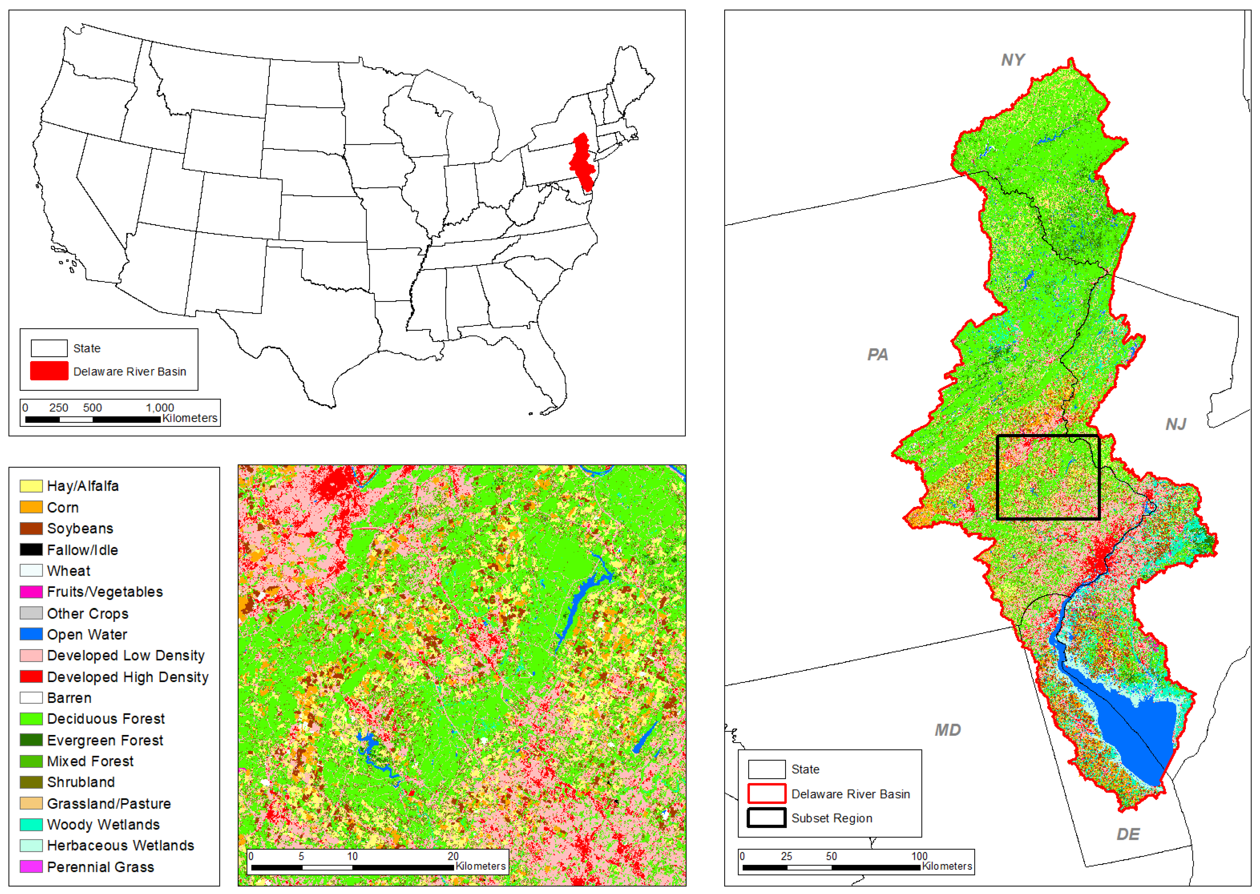
The DRB is an active area of focus for US Geological Survey (USGS) research activities, making it an ideal test bed for the development of a long-term landscape time series (Figure 1). The spatial coverage of the study area was defined from the watersheds defined in the Watershed Boundary Dataset component of the USGS National Hydrography Dataset (Hydrologic Unit Codes 020401 and 020402, [25]). The DRB is small yet ecologically diverse and provides drinking water to ~15 million people in the watershed and surrounding areas. Based on the most recent NLCD product (NLCD 2016), ~20% of the region is currently developed, with another ~15% used for agricultural purposes [10]. Societal concerns in the region include the historic impacts of drought, including events such as the 1960s “drought of the century” that resulted in low water flows and saltwater intrusion in the estuary that threatened drinking water supplies for Philadelphia, Pa; New York City, NY; Camden, NJ; and other urban centers [26,27]. The timing of this drought precludes the use of direct Landsat observations for characterizing historical LULC. Historical change in anthropogenic land use has had strong impacts on water resources in the region, while anticipated future land use and climate change are likely to further stress those resources [28]. The long-term landscape time series developed here will be used to explore historical relationships between land use, water use, and drought, as well as facilitate future water resource planning in the region.

2.2. Initial Conditions and Modeling Parameters

Here, we lay the foundation for potential broader-scale application at the national scale by prototyping DRB-specific land cover backcasting datasets to the year 1680 (determined to be “pre-settlement” as described in Section 2.5 below) and forecasting datasets to the year 2100. All land cover modeling was completed at 10-year intervals, at a 30-m spatial resolution, and for 20 thematic land cover categories (Table 1). FORE-SCE can run at any temporal time step, but 10-year intervals were selected due to computational constraints imposed by higher temporal resolutions. The 10-year analysis interval is also consistent with recent applications of the FORE-SCE model in the Great Plains [13,23]. A 30-m spatial resolution is a substantial improvement over past national-scale applications of FORE-SCE which were modeled at 250-m [21,22]. The selected 30-m resolution also provides consistency with widely used, national-scale datasets such as NLCD and CDL. Thematic classes represent most classes from the 2016 NLCD [10], with NLCD’s “cultivated cropland” class further differentiated into major crop types in the region from CDL data [24]. To maintain thematic consistency with land cover modeling work underway in adjacent regions 2018-era CDL data were used and the crop category tobacco, though not present in DRB scenarios, remains in the classification schema. The four NLCD classes related to urban development density were collapsed into two classes, a “low-intensity” class and a “medium/high intensity” class. Forecasting was conducted under seven socioeconomic scenarios and three climate projections, resulting in 21 total future landscape projections (Section 2.6.1).

2.3. FORE-SCE Structure

The structure of the FORE-SCE version used here mimics the overall “demand” and “spatial allocation” paradigm from recent FORE-SCE applications [13,23], with substantial model updates as we note below. The primary driver in the FORE-SCE workflow is a temporal series of quantitative change prescriptions for each LULC category in a specific geographic region, known as demand. Spatial allocation algorithms ingest demand at the regional scale and place pixels and parcels of change on the landscape until demand for a given scenario and timestep is met. The same model paradigm exists for both historical landscape reconstruction, and for future projections, with a requirement for regional-level demand (with a region consisting of any geographic framework, such as by state, ecoregion, or watershed), and subsequent spatial allocation to create spatially explicit LULC maps at requisite time intervals. However, given the unique nature of temporal LULC change characteristics when reconstructing historical landscapes versus projecting future landscapes, model function and parameterization differ depending upon temporal trajectory, as noted in Section 2.5 and Section 2.6 below, respectively. The primary objective of FORE-SCE is to represent any scenario of prescribed landscape change with the highest degrees of spatial and thematic resolutions and pattern fidelity as possible.
A key element of the spatial allocation algorithms are suitability surfaces which quantify, for a given pixel, the probability of each LULC class occurrence. Suitability surfaces play a key role in driving where change occurs on the landscape. Suitability surfaces can also be dynamic through time, with past applications updating suitability surfaces in lockstep with projected changes in climate or water availability [13]. The spatial allocation of prescribed change is implemented at either the pixel- or patch-level. Patch-level change refers to land cover transitions that occur in discrete, contiguous groups of pixels, often corresponding with anthropogenic activity. Pixel-level change typically corresponds with natural vegetation land covers and does not employ discretely defined units.
Patch-level change is further divided into two styles: randomly generated patches and predefined ownership-based parcels. Allocation style is defined for each LULC class and may be modified dependent on region and scenario (Table 1). The use of ownership-based parcels ensures realistic representation of landscape pattern changes at fine spatial scales, but the parcel data themselves are unavailable to FORE-SCE data users due to privacy and distribution restrictions. Parcels for the DRB are derived from three sources, as no one parcel dataset provided adequate ownership and management information for all land use sectors:
  • USDA Common Land Unit (CLU) data were used as the primary dataset to represent agricultural land management parcels [29];
  • Agricultural parcels extracted from Landsat data by Yan and Roy [30] were used to augment CLU data and fill in gaps where CLU data were unavailable;
  • Parcels from the Homeland Infrastructure Foundational-Level Data provided ownership parcels for urban and other non-agricultural lands [31].
FORE-SCE accounts for the complete suite of LULC classes found on the landscape. The driver of change for “demand” is primarily assumed to be anthropogenic change, with natural land types responding to changes in anthropogenic land use related to urban development, agriculture, forestry, mining, and reservoir construction. These are also the land use and land cover classes for which both historical data and future scenarios are much more widely available, with information on trends and spatial distribution of natural land covers much more difficult to acquire. FORE-SCE thus maintains a flexible status for land cover classes without explicit prescriptions for change. For example, in a scenario calling for agricultural expansion, natural vegetation categories (e.g., grassland, shrubland, forest) in locations that satisfy suitability requirements for cropland will convert to agricultural categories. For scenarios exploring a contraction of agriculture, natural vegetation classes will increase and flexibly displace crop categories as needed. Flexibility is defined at the class level and dependent on region and scenario. For instance, grassland/pasture was supplied with explicitly prescribed change for historical backcasting but allowed to respond flexibly to other classes for future scenarios. Classes with explicitly prescribed change are further addressed in Section 3.4.
Natural vegetation can also change over time even in the absence of anthropogenic driving forces. Dynamic suitability surfaces drive shifts in the distributions and proportions of natural vegetation classes including grassland, shrubland, and forest classes. Tied to projected changes in climate input into FORE-SCE, pixels of these classes that are characterized as “unsuitable” to support a given cover class under new climate conditions may shift to more suitable classes, as described by Sohl et al. in 2019 [13].
Additional details about the overall FORE-SCE paradigm and structure can be found in prior publications [13,22,23]. What follows are new FORE-SCE developments applied to the DRB (Section 2.4), specific modeling methodologies for both historical landscape reconstruction (Section 2.5) and future projections (Section 2.6) in the DRB.

2.4. FORE-SCE Improvements for Delaware Basin Application

The general FORE-SCE structure and paradigm above was suitable for both historical landscape reconstruction and future scenario modeling in the DRB. However, a number of enhancements and new modeling elements were developed to improve model performance in the basin, while other modifications were made to improve model flexibility and automation, as we aim to apply this framework across the conterminous US.

2.4.1. Urban Module Advances

The FORE-SCE urban module operates similarly to a cellular automata model, with urban growth patterns empirically dependent upon the existing urban pattern and growth elements that can mimic both edge and spontaneous urban center growth. A priority is placed on edge growth from existing urban pixels (including road networks), with urban growth prioritized for existing high-density urban areas, but model parameters also create opportunities for smaller urban areas to coalesce or for development to leapfrog from larger urban areas to smaller, more rural areas. Prior work has demonstrated that this approach produced results more consistent with theoretical, long-term patterns of urban growth [13].
Additional advances in FORE-SCE’s urban module used in the DRB include the following:
  • Development of capabilities for the urban change module to operate over descending time steps, supporting historical backcasting;
  • Flexibility in parameterization, permitting users to supply spatially explicit likelihood datasets that influence urban change;
  • Support of land cover category schemas containing multiple urban classes (past FORE-SCE applications modeled a single urban class).
These modifications facilitate historical backcasting reconstruction and improve the functionality and flexibility of modeling future scenarios. For example, the addition of ancillary data that influence the spatial allocation of change allows for the use of historical data to guide the removal of urban features as the model operates in reverse, replicating actual historical landscape patterns. Support for multiple classes enables transitions between urban intensity levels over time.

2.4.2. Improving Automation and Stochasticity

Suitability surfaces are a key element in converting quantitative demand into spatially explicit land cover realizations [13]. These surfaces are derived by mapping the likelihood-of-presence resulting from stepwise logistic regression using biophysical and anthropogenic covariates and initial land cover conditions (i.e., 2018-CDL), [22] and are utilized by the model to establish “growth zones”, spatial zones where change in a given land cover class is most likely to occur [13]. Prior to this application, the establishment of those class-by-class zones was often an iterative process, requiring interpreter intervention and analysis, potentially introducing subjectivity to the process. The need for a more objective process necessitated the development of new, more automated methodologies for generating suitability surfaces and establishing spatial zones of potential change. This methodology is expected to scale up towards the national scale.
A new methodology was developed that: (1) reduces interpreter intervention, (2) automates establishment of spatial zones of change, and (3) enhances model stochasticity by using initial landscape conditions and weighted random selection to automatically calibrate and establish spatial-growth zones for each class. Figure 2 demonstrates this new process for the land cover category “corn” (Table 1) in a 54 km × 54 km subregion northeast of Pennsylvania (Figure 1, bottom left). Initial land cover class presence/absence and corresponding suitability values (Figure 2a,b, respectively) are used to generate the total operating characteristic (TOC) curve (Figure 2c) for each land cover category [32]. The TOC curve explicitly reveals the quantities of correctly predicted presence (true positives) (TP), correctly predicted absence (true negatives) (TN), incorrectly predicted presence (false positives) (FP), and incorrectly predicted absence (false negatives) (FN) for all possible suitability thresholds of a given category. The maximum and minimum boundaries of the plot define the space of diagnostic potential. Sensitivity (Equation (1)) and specificity (Equation (2)) are computed by dividing TP by the number of actual pixels in the initial landscape with category present (P) and TN by the number of actual pixels with category absent (N).
Sensitivity   ( True   Positive   rate ) = TP P
Specificity   ( True   Negative   rate ) = TN N
The threshold maximizing the sum of sensitivity and specificity (MSPS) for the category is then computed. In Figure 2d the category’s underlying suitability values for its initial condition of presence is plotted as a histogram along with MSPS. For land covers prescribed to increase on the landscape, an iterative process of random selection centered on MSPS converges on a selection of pixels with a suitability-value distribution that is similar in shape to the category’s starting condition. The selection is from pixels that do not correspond with class presence and therefore represents the spatial extent of potential expansion for the given class. In Figure 2e the histogram for all eligible expansion pixels (those where the given class is absent) is displayed in green (note: pixel counts for very low-suitability values exceed y-axis plotting limits). Pixels for expansion selected from all eligible pixels under the (1) manual percentile-cutoff method and (2) the new automated method are plotted (pink and brown, respectively). Note: suitability values are relative to each land cover category and are not used as raw prediction values when establishing growth zones.

2.5. Historical Reconstruction: 1680–2018

FORE-SCE was used in a “backcasting” mode to iteratively reconstruct landscape change from our starting 2018 date backward to 1680, at 10-year intervals. We selected 1680 to represent “pre-settlement” vegetation in the region, as the first European settlement in the DRB did not occur until 1631, and impact on pre-settlement vegetation was deemed to be negligible prior to 1680 [33,34]. There is also a lack of useful population, agricultural land use, or other historical data sources related to landscape change prior to 1680.
As with past FORE-SCE applications, long-term historical reconstruction is based on quantifying regional demand for modeled timesteps with spatial allocation to produce spatially explicit maps. Regional demand, in turn, is based on the acquisition and harmonization of historical data sources quantifying regional LULC change. With a goal to develop a methodology that was extensible and scalable to other regions of the US, we relied on data sources for historical landscape reconstruction that were consistent and nationally available.

2.5.1. Establishing Pre-Settlement Vegetation

The LANDFIRE Biophysical Settings (BPS) dataset [11] represents vegetation most likely to have been prevalent prior to Euro-American settlement (i.e., 1680) and provides consistent data at our 30-m spatial resolution. We recoded the LANDFIRE BPS dataset for the DRB to match our categorical schema (Table 1) and used the resulting dataset as a pre-settlement target for historical landscape reconstruction. As FORE-SCE models backward in time towards a historical end year before Euro-American influence, anthropogenic landscape features (i.e., cropland, urban, reservoirs) eventually transition to pre-settlement vegetation types. The rate, pattern, and spatial distribution of change, as “current” (2018) landscape conditions revert to pre-settlement conditions, are driven by a variety of historical data sources for the region, as explained in Section 2.5.2 below.

2.5.2. Establishing Historical Demand

Agricultural and urban land uses generally have the most information available historically and serve as the backbone of the historical reconstruction process. These and select other anthropogenic land uses are actively modeled within FORE-SCE, while non-anthropogenic, “natural” vegetative covers such as grassland, shrubland, and forest are passively modeled as described in Section 2.3. Below, historical demands for FORE-SCE applications are described in terms of agricultural and urban demand.

Agricultural Demand

The demand for historical change for agricultural classes was derived using Agricultural Census records [35] and historical population and labor force information [36,37,38]. The Agricultural Census provides county-level estimates for crop production beginning in 1840. Crop acreage estimates, however, were not introduced until 1880. From 1840–1870 Agricultural Census estimates consisted of crop yields. County-level acreages provided by the census were aggregated to match modeled thematic classes and converted to pixel-level prescriptions of change. Interpolation was used to estimate acreage for years in which crops of interest were absent from the census. Extrapolation was used to estimate acreage for census years from 1840–1870. Population and labor force data corresponding with Agricultural Census acreages were used to compute acres-per-crop-laborer. This relationship could then be used to derive acreage using estimated labor population for the years prior to the Agricultural Census (1680–1830).

Urban Demand

Developing the historical demand for urbanization required harmonization of multiple historical data sources, with substantial disagreement on rates of historical urban change. The Historical Settlement Data Compilation for the United States (HISDAC-US) is derived from historical property records and provides temporal (five-year increments) gridded (250-m resolution) settlement data between 1810 and 2015 for the conterminous United States [39]. The HISDAC-US First Built-up Year layer provides the first recorded year a structure was built within a given cell extent. Another dataset on historical urban change is the US Census American Community Survey (ACS) with five-year estimates that include census block group-level median year-built estimates for building structures [40]. While neither of these two historical datasets directly indicate when a given spatial unit would have been classified as “urban”, they can both be used to generate independent estimates for historical urbanization trends, as follows.
Year-built pixel counts were based on all urban land cover pixels present in the model’s initial (2018) land cover and then converted to cumulative urban land cover pixel counts where each year’s cumulative value is the sum of all urban pixels with a year-built less than or equal to the given year. Plotting cumulative urban pixel counts against historical source year-built values (median for ACS and first year for HISDAC-US) reveals curves that are well fit by logistic growth functions and estimate urbanization trends for the region (Figure 3a). ACS cumulative urban pixel counts suggest a more abrupt historical growth rate for the region than do the HISDAC-US counts. This observed trend is likely due to the influence of urban redevelopment within some ACS block groups. Block groups experiencing large amounts of redevelopment of existing urban cover are represented with a temporal shift forward of median year-built and original structure-built dates are lost as redevelopment occurs. Conversely, the HISDAC-US may underestimate the timing of urbanization as “first built-up year” may precede the year at which a pixel would be considered “urban” in our thematic classification system.
Cumulative population [36,37] plotted on the same time interval (using the left vertical axis) reveals a logistic growth curve more similar in shape to HISDAC-US than to ACS according to the comparison of their logistic growth steepness factors (Figure 3a). To further assess both historical data sources, urban areas from the USGS Historical Topographic Map Collection were manually digitized to estimate urban cover for the year 1900 [41]. The estimation of total urban cover for 1900 from historical topographic maps lies between the cumulative growth curve fits for HISDAC-US and ACS (Figure 3b, red square). We also compared HISDAC-US and ACS data with urban land cover quantities as mapped by contemporary remote-sensing-based land cover classifications. Remotely-sensed urban pixel counts were derived from the Land Change Monitoring, Assessment, and Projection (LCMAP) time series for years 1985 and 2000 [12] and from the NLCD for 2016 [10] (Figure 3b).
Ultimately, we selected a harmonization approach to incorporate both HISDAC-US and ACS in the derivation of urban land cover estimates for backcast land cover modeling. A third logistic growth model of cumulative urban land cover quantity was fit using both sets of historical time series data (Figure 3b, green curve). The fit is weighted more heavily to HISDAC-US as that dataset provides a curve more consistent to overall population trends and provides a broader temporal range of data points. The final, harmonized logistic growth curve was used to estimate the total urban land cover area for each backcasting 10-year interval. To separate historical urban change into the low- and high-intensity categories, we assumed a simple, constant rate of change between categories. The rate of conversion between urban types was then solved to arrive at known proportions in the model’s initial land cover conditions, assuming pre-settlement conditions of no urban land cover. The conversion rate was then applied to calculate the amount one urban category is expected to transition to another for any modeled time interval. Demand used by the model to spatially allocate prescribed change for a given category is then simply the difference in category quantity estimates between subsequent backcasting time steps.

Other Demand

Agricultural and urban demand are the two largest anthropogenic land use impacts in the DRB, but demand for other land cover classes was also included. Temporal and spatially explicit information on wetlands is lacking in the DRB, but coarser-scale information provided guidance for aggregate demand across the watershed. We used drained land information from the US Census of Agriculture (1920–1960) [42,43,44,45] and a US Fish and Wildlife Service report to Congress on wetland loss (1780–1980) [46] to characterize historical change. With LANDFIRE BPS serving as the pre-settlement historical endpoint, wetland quantities for historical reconstruction years without reported estimates could be interpolated.
The establishment of reservoirs over the historical 1680 to 2018 period also served as a form of “demand”, with the need to remove reservoirs as the model iterated backward in time. A separate methodology for reservoir removal (and subsequent replacement with other land covers) was established in the spatial allocation element of FORE-SCE, as described in Section 2.5.3 below. Natural land cover classes (e.g., forest, shrubland, and grassland classes) are not provided an explicitly prescribed demand within FORE-SCE and instead are treated as “passively” modeled land covers that respond to prescribed changes in anthropogenic land use activity, as described in Section 2.5.3 below.
Table A1 of Appendix A provides a summary of the historical datasets used in the application, including time period, resolution, and internal accuracy assessment.

2.5.3. Historical Spatial Allocation

Data to support historical backcasting are often not abundant and are generally spatially coarse, but our spatial allocation process is able to incorporate that information to produce spatially explicit land cover maps consistent with the starting 2018 land cover data. For historical backcasting, the landscape is altered for 10-year intervals from 2018 backward to 1680, with a target endpoint of “pre-settlement” vegetation as defined by the LANDFIRE BPS data. Demand for anthropogenic land covers was developed based on multiple historical data sources, with land covers such as the two urban classes and eight agricultural classes eventually disappearing from the landscape as we meet pre-settlement conditions (Section 2.5.2). Natural land cover classes are “passively” modeled, replacing “lost” anthropogenic land cover classes as the model iterates backward in time, eventually converging on pre-settlement vegetation (Section 2.3).
Suitability surfaces used to guide the spatial allocation of change can be dynamic over time (Section 2.3). While suitability surfaces for future scenario-based projections have typically been parameterized to respond to corresponding projected changes in climate or water availability, suitability surfaces for historical backcasting were parameterized to effectively calibrate to existing historical data. For example, the finest-scale long-term historical data available for agricultural classes were county-level Agricultural Census data. Those data were used to not only construct “demand” (Section 2.5.2) but also to modify our starting point, contemporary suitability surfaces to create historically dynamic suitability surfaces for agricultural classes. The modified, 1850–1997 Agricultural Census data developed by Waisanen and Bliss [47] were used to modify historical suitability surfaces for agricultural classes, improving the ability of the model to match historical distributions of individual crop types. The time series of agricultural development provides county-level proportions of harmonized total “improved farmland”. A contemporary land-in-agriculture ratio was computed and included among covariates in the initial regression model. Following the same process used to derive dynamic suitability surfaces for forecasting scenarios described by Sohl et al. [48], dynamic backcasting suitability surfaces were derived by substituting the historical ratios for the contemporary ratios before mapping the regression parameters over the covariates to produce spatially explicit suitability values.
Similarly, coarse-scale historical data can be used to help guide the spatial allocation of urban lands as the model iterates backward in time. The HISDAC-US Built-up Intensity (BUI) product provides indoor-building gross-area sums (square meters) per grid cell (250 m) at five-year increments from 1810 to 2015 [39]. For backcasting the years in which HISDAC-US data were available, normalized moving-window sums of historical BUI were used to weigh the selection of pixels most likely to experience transition. This increases the likelihood that modeled urban decline is most likely to occur where historical BUI was lowest.
Another anthropogenic land use accounted for in the historical modeling is reservoir construction. We developed a semiautomated process that utilizes the National Inventory of Dams [49] and extracts reservoirs from the initial land cover, labeling them with the construction year of the associated dam. We added to the FORE-SCE model the capability to use labeled reservoir datasets as change patches to transition reservoirs to dominant local natural vegetation. We employed the new capability to remove reservoirs from the landscape during historical backcasting, replacing “water” land cover associated with a reservoir with suitable upland land cover classes at the first 10-year interval prior to the recorded dam construction date. The reservoir replacement class is determined by the majority natural cover within a variable buffer around the feature (we used 90 m for the DRB). The methodology described here was used for historical landscape reconstruction but could also support forecasting scenarios that include reservoir removal.

2.6. Future Projections: 2018–2100

Future projections are more straightforward than historical reconstruction, with the basic FORE-SCE structure (Section 2.3) and the recent model improvements (Section 2.4) capable of addressing modeling needs in the region. To facilitate long-term analyses related to the impacts of landscape change, model runs were done from current (2018) to 2100, with nominal 10-year intervals that match the historical backcasting intervals. A scenario-based approach was used to develop and visualize a variety of future landscape futures, facilitating the exploration of uncertainties related to future landscape change.

2.6.1. Scenario-Based Demand

As with historical backcasting, FORE-SCE requires quantitative demand for each modeled land cover class for each future modeled time interval. Several different approaches were used to construct demand for past FORE-SCE applications including: (1) straightforward “business-as-usual” (BAU) scenarios extrapolated recent trends (typically derived from remote-sensing-based LULC databases such as NLCD), and (2) downscaling of existing, coarse resolution scenarios, or custom econometric scenarios. Demand may also be constructed in partnership with regional stakeholders by exploring “what-if” scenarios that facilitate visualization of landscape outcomes for various policies.
DRB scenario development followed a similar process to that employed for recent model applications of FORE-SCE in the Great Plains [13,23]. Table 2 describes the seven individual scenarios that were modeled, based on three different sources. The BAU scenario extends recent trends from two different sources, with trends in individual crop categories based on recent trends between the 2008 and 2018 dates of the USDA CDL data, with all other land cover classes based on extrapolated trends between the 2001 and 2016 NLCD dates. Three scenarios were based on the US Department of Energy Billion Ton Update (BTU) [50], which provides a county-level exploration of the impacts of various economic scenarios on the agricultural landscape. The BTU scenarios are based on variations in modeled farmgate prices for biomass for biofuel production. The final three scenarios were derived from the Global Change Assessment Model (GCAM), with GCAM annual land cover percentages at 0.5-degree resolution downscaled to finer resolutions to support regional and national applications in the United States [51]. West et al. provide three GCAM scenarios to explore a range of human effort to mitigate climate change—a reference scenario provides landscape conditions with the assumption of no targeted climate-change mitigation efforts, while two additional scenarios assume mitigation efforts necessary to achieve total radiative forcing levels of 2.6 and 4.5 W/m2 by the year 2100, respectively. Sohl et al. [13] provide additional information on development of BAU, BTU, and GCAM scenarios.

2.6.2. Projected Spatial Allocation

Spatial allocation of the scenarios described above largely follows the paradigm used for the recent Great Plains application [13] and is described in Section 2.3, with the addition of new modeling elements described in Section 2.4. The new urban model was applied for the two urban density classes described in Table 1. As with past applications [13,23,48], projected climate information was incorporated into future projection modeling. Downscaled temperature and precipitation projections [52] averaged from multiple Coupled Model Intercomparison Project Phase 5 (CMIP5) models (Table A2) were used to generate dynamic suitability surfaces sensitive to multiple projected climate change pathways. Pixel-level suitability for a given LULC class thus evolves over time, with LULC classes expanding, contracting, or shifting in space in response to projected changes in climate.

2.7. Model Assessment

FORE-SCE model performance was evaluated at multiple levels:
  • Inter-scenario model comparison—We examine differences between modeled land cover over the same time intervals under different scenarios.
  • Intra-scenario model performance—We assess FORE-SCE’s internal abilities to represent prescribed change (demand) in a modeled land cover realization for a given future scenario and to spatially match observed change between two reference LULC datasets, NLCD 2001 and NLCD 2016.
  • Historical reference—We compare modeled land cover with spatially-explicit historical references.
  • Cross-model scenario comparison—We compare FORE-SCE’s simulation of land cover change to the simulations produced by a suite of global IAMs.
As with past applications, the concepts of quantity and allocation disagreement were used to evaluate model results [53]. Quantity disagreement is the amount of difference between model results and a reference dataset arising from variances in overall proportions of landscape categories. Allocation disagreement results from an imperfect match in the spatial arrangement of landscape elements. Allocation disagreement can be further divided into the categories exchange and shift. Exchange spatial disagreement is the difference between two categories in which one location corresponds with the reverse in another location. Shift disagreement entails spatial differences between more than two categories [54].
To track the model’s ability to represent prescribed change (demand) on the landscape, we computed the absolute deviation (both positive and negative) of modeled change from the prescribed change at every timestep, for every land cover category that has explicitly supplied demand. This procedure was conducted for all scenarios and summarized across modeled time intervals.
Applying the FORE-SCE model to historical land cover reconstruction requires additional parameterization and the flexibility to use what is available from limited historical reference data. As described above, we made use of historical datasets [39,47] to guide the spatial allocation of agricultural and urban land cover categories. To assess the impact of incorporating these historical datasets on resulting patterns we employed tandem model runs. These runs are identically parameterized other than the historical parameter of interest and serve to isolate the effect of the varying parameter. We quantify and examine the effects below.
Hurtt et al. [19] have produced Land Use Harmonization (LUH2) datasets to smoothly connect historical data from the History of the Global Environment database (850–2015) and multiple alternative future scenarios represented by IAMs (2015–2100). We compare the trends of aggregated categories modeled by FORE-SCE for historical reconstruction and multiple future scenarios to their counterparts as represented by LUH2.

3. Results

The overarching goal was to produce consistent, long-term, historical, current, and future representations of landscape change, with one historical landscape reconstruction that strove to match reference data as closely as possible, and multiple future scenarios to represent the considerable uncertainties.

3.1. Modeled Trends for Aggregated Categories

Figure 4 depicts temporal trends of modeled results for the DRB from 1680 through 2100, depicting trends in major, aggregated land cover classes, including the two biggest anthropogenic driving forces of change in the region (agriculture and urban), and the largest “passively modeled” natural vegetation class (forest). Agricultural land covers increased steadily for the first two centuries from the starting 1680 pre-settlement land cover, plateauing in the latter half of the 19th century and peaking near the turn of the century, before declining in extent from about 1920 onwards. As agriculture started to decline, the rate of urbanization dramatically rose, rising steadily until the present day. Forested lands decreased sharply in the 19th century in response to agricultural expansion, with reforestation occurring until about 1970 as marginal agricultural lands were then abandoned. However, forests again began to lose area after 1970, as agricultural abandonment abated and urbanization continued a strong increase. The U-shaped pattern of forest decline and subsequent rebound from 1680 to 1970 is consistent with forest transition theory [55]. The renewed declines in forest area after the 1970s fit the pattern of a “contemporary regressive stage” of forest transition found for the Eastern US as a whole during this time period, driven by land use intensification, urban expansion, and diminution in processes of agricultural abandonment and reforestation [56]. The aggregated categories simplify the visualization of trends and together comprise the majority of the DRB’s initial landscape (83%).
Projected land cover trends from 2018 to 2100 show substantial variability among scenarios, yet none of the scenarios anticipate volatility approaching that of 20th-century landscape change in the DRB. The BAU scenario is the most dynamic, with extrapolations of recent trends resulting in offsetting trends of strong declines in agricultural land, and continued expansion of urbanized lands, with relatively stable forested lands. Other scenarios show similar trends in agriculture and urban but with lower rates of urban growth, with the exception of the GCAM Reference scenario where agricultural lands increase. Overall, as described in Sohl et al. [57], there tends to be more similarity within a scenario family than between them. For example, changes in agriculture for the three GCAM scenarios are all clustered more closely to “no-change”, while the three BTU scenarios all show higher agricultural loss than any GCAM scenario. Similarly, BTU scenarios tend to show higher forest increases than most of the GCAM scenarios. However, across all scenarios, substantial variability exists in modeled landscape trends (as described in the next section), facilitating analyses of the uncertainties associated with landscape change impacts on human and natural systems.

3.2. Examining Scenarios in a Subregion

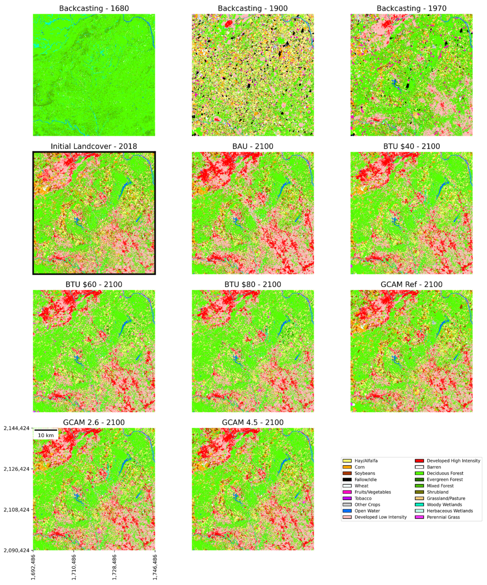
Figure 5 displays initial land cover conditions, all forecast scenarios at the year 2100, and three backcasting dates for the same subregion in Figure 1. In each image, we observe the interplay of agricultural and urban anthropogenic classes with the dominant natural vegetation, forest classes. Historical landscape reconstructions spatially depict the patterns described in Section 3.1. The historical landscape at “pre-settlement” in 1680 is dominated by deciduous and mixed forest, while a substantial proportion of forest was cut by the time the region as a whole reached peak agricultural extent near the start of the 20th century. From 1900 to 1970, marginal agricultural lands throughout much of the region were abandoned and allowed to regenerate back into forests, leaving much smaller pockets of higher-value cropland within the growing forest mosaic. Urban lands increased dramatically during the 20th century as shown in the northern part of the image.
Most forecasting scenarios generally agree on trends in urban expansion and agricultural decline. The displacement of agriculture by forest is most prevalent in the BTU $60 and $80 scenarios which, despite prescribing modest growth for perennial grass (associated with assumptions on cellulosic biofuel production in those scenarios), forecast general agricultural decline. As noted above, the GCAM Ref scenario stands alone in its prescription for agricultural gains, as it is a scenario without any assumptions on climate mitigation and thus less likely to convert marginal agricultural lands to forests. The BAU scenario maintains urban expansion at rates which the other forecasting scenarios taper.

3.3. Assessing Inter-Scenario Variability with Difference Metrics

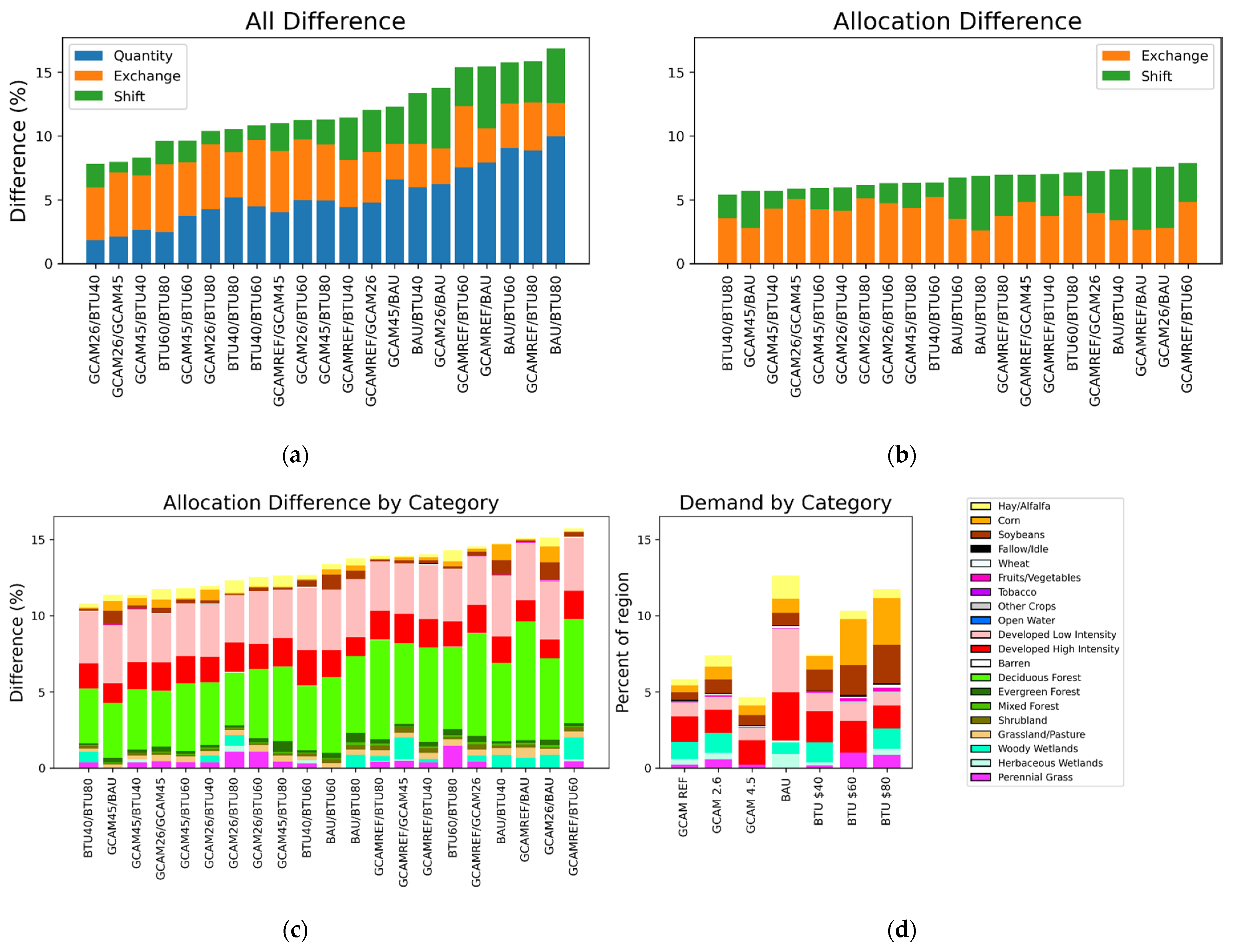
Figure 6 shows the components of quantity difference and allocation difference (including “exchange” and “shift” components) for every future scenario combination across the forecast period. We expect to see quantity difference between scenarios as, by definition, a scenario contains prescriptions of quantitative change that differentiate it from other scenarios. We also expect to see allocation difference. Quantity difference without any allocation difference between different scenarios would indicate that the modeled projections result from a completely deterministic, non-stochastic process of spatial allocation. Whereas, high levels of allocation difference in relation to prescribed change may suggest that the model is poorly calibrated or highly random.
Not surprisingly, we observe consistent, increasing trends in difference for all pairs of scenarios as they are modeled into the future. The difference present by the year 2100 is largely cumulative given that most changing land cover categories trend in one direction under forecast scenarios. Figure 7a charts all components of difference for the final year of projection (2100), when scenarios have fully diverged, and the difference is at its highest. Figure 7b isolates the spatial components of difference described above and Figure 7c separates allocation difference for the final forecast year into its land cover category components. Note: considering allocation difference separated by category results in each pixel in the difference being counted twice—once for each different category in the pair—the actual total allocation difference across the region is thereby half of the allocation difference summed across categories. The bars in Figure 7c are thereby twice the height of the actual allocation difference bars in Figure 7b.
For the projected year 2100, the total allocation difference across all category combinations ranges from 5.4% to 8.5% of all the region pixels (Figure 7b). On average, “exchange” represents a majority of allocation difference when total allocation difference is lower, while “shift” on average grows as a proportion of total allocation difference when total difference itself increases. The land cover categories contributing most to allocation difference are both low- and high-intensity developed classes and deciduous forest (Figure 7c, pink, red, and green, respectively). This is consistent across all scenario comparisons and reflects the high degree of potential spatial variability present in the urban-to-non-urban interface.
Figure 7d shows total absolute demand (both prescribed gain and loss) separated by land cover category and plotted by scenario as a proportion of the region. BAU and GCAM 4.5 prescribed the highest amounts of change, respectively. The contribution of agriculture land cover categories to allocation differences is relatively minor in comparison to the contribution of urban categories when prescribed absolute change is considered. As described above, both agriculture and urban change are parcel-based and guided by suitability surfaces. However, the urban module enacts change (be it growth or decline) at the urban-to-non-urban interface and here finds more opportunities for divergence between scenarios than does agricultural change. This results in distinct urban patterns between scenarios with a less overall agreement.

3.4. Modeled vs. Prescribed Change (Demand)

3.4.1. Backcasting Assessment

The absolute deviation of modeled quantities from prescribed demand summed over all years of historical backcasting is approximately 0.94% (Table 3). In Figure 8, each land cover category’s modeled outcomes are plotted against the corresponding demand for each year of backcasting. The passive, flexible land cover categories have no explicit demand and instead respond to prescribed demand in the anthropogenic land cover classes. Demand for these classes is thus plotted as a horizontal line representing the initial quantity.
The region’s historical trends in agriculture see a peak near the year 1900. Passive, natural vegetation classes experience a corresponding trough in quantity but grow to dominate the landscape by pre-settlement. Urban categories are reduced to zero by pre-settlement. Notably, prescribed demand for urban categories representing low- and high-intensity development does not include urban land cover representing roads. The deviation between prescribed demand and modeled change that is apparent in the plot for urban/developed categories is due to the aforementioned removal of roads, which the model conducts under prescriptions of urban decline but which is not explicitly represented in the prescribed demand. For this reason, urban categories are omitted in the overall assessment of deviation from demand (Table 4).
Woody Wetlands are present in the pre-settlement natural vegetation dataset based on LANDFIRE BPS. However, Herbaceous Wetlands are not. Woody Wetlands were left flexible and allowed to displace anthropogenic classes as necessary, whereas prescribed change was supplied for Herbaceous Wetlands to reach pre-settlement levels.

3.4.2. Forecasting Assessment

Table 5 displays deviation from demand for the seven forecasting scenarios under RCP-average climate assumptions. Overall, for six of the scenarios, the total modeled change deviates from prescribed demand by less than 1%. The GCAM Ref scenario stands out with ~1.12% deviation from the prescribed demand. Notably, this scenario is the only forecasting scenario prescribing net gains for aggregated crop classes (Figure 4). Overall, FORE-SCE excels at matching prescribed demand, and thus quantity difference for prescribed scenario land cover.
The FORE-SCE model can use pre-processed ownership parcels to represent anthropogenic change on the landscape, which results in more realistic patterns at higher spatial resolutions [13]. However, when a category expands into a new area, it may do so via parcels that have not historically been of the expanding land cover type and struggle to replicate historical patterns. We observe that the categories contributing most to deviation from demand for the GCAM Ref scenario are agriculture categories that miss prescribed growth (both overshooting and undershooting) due to reliance on coarse, overly-large ownership parcels. This is specifically observable for the Perennial Grass category across BTU and GCAM scenarios, which all call for growth and primarily see expansion among large ownership parcels, as these are the only “suitable” parcels for the class to occupy. FORE-SCE currently does not account for the potential land ownership parcels to evolve over time (e.g., subdivision of a large agricultural lot as urban centers expand). Automating the development of ownership boundaries that vary in size and shape under different scenarios is an active area of research for the project.

3.5. Modeled vs. Contemporary Reference

Using NLCD 2001 as the starting point, we modeled land cover quantity changes from 2001 to 2016 in a single 15-year time interval for the DRB. Observed quantity changes for all categories between 2001 and 2016 in the NLCD datasets served as FORE-SCE’s demand input. The model’s simulated 2016 land cover dataset was then compared to the reference NLCD 2016 land cover to assess FORE-SCE’s ability to maintain spatial allocation integrity between reference points inside the remote sensing period of record.
FORE-SCE’s simulation of 2016 NLCD change finds total pixel-level agreement/disagreement at 95.00%/5.00% against the 2016 NLCD reference dataset (Table 5). As observed in Section 3.4.1 and Section 3.4.2 the model closely matches prescribed changes at the category quantity level. Here quantity represents 0.65% of all disagreement. Allocation disagreement represents almost all the difference between the modeled and reference 2016 datasets and is split approximately evenly between the spatial components exchange and shift. We consider this result an appropriate reflection of the stochasticity inherent in the interface between anthropogenic and natural land covers and validation of FORE-SCE’s ability to model with high spatial fidelity in the region.

3.6. Modeled vs. Historical References

3.6.1. Modeled vs. Historical Agriculture

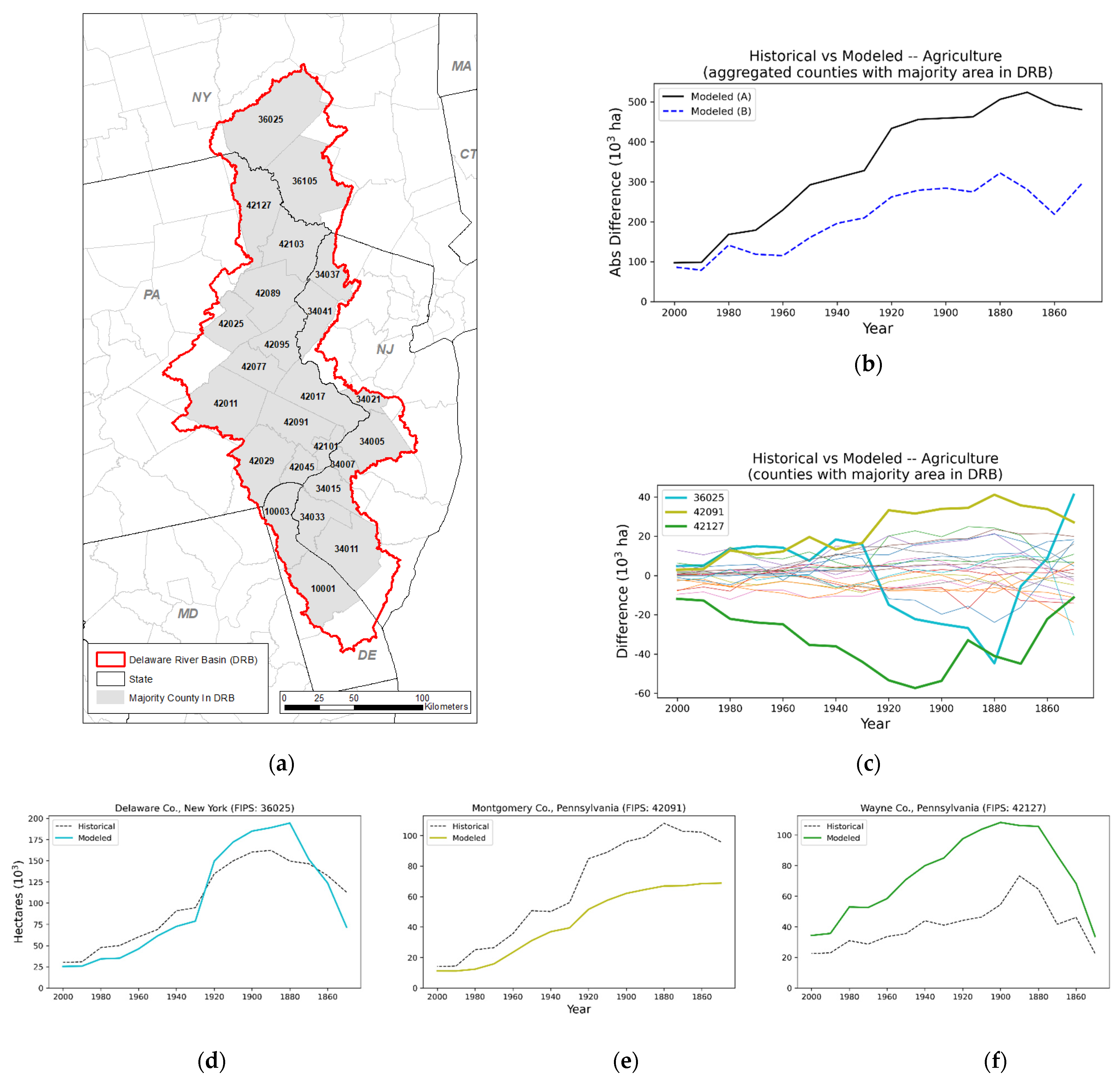
Section 3.4.1 and Section 3.4.2 demonstrate FORE-SCE’s ability to meet overall demand for a region, but options for assessing the model’s ability to accurately represent historical landscape patterns at finer scales are limited, given the lack of spatially explicit, historical land cover data (the reason this modeling work is necessary). We can do some comparisons with our finest-scale available data, which for many historical datasets is county-based. We modified suitability surfaces using historical county-level agricultural time series (described above) with the goal of improving the spatial allocation of agricultural classes in backcasting. Below we compare the resulting county-level modeled area-in-agriculture to the historical time series dataset for two backcasting model runs: model run A without historically dynamic suitability surfaces and model run B with historically dynamic surfaces.
For comparison purposes, the modeled crop categories were aggregated to match the Agricultural Census data’s generalized class “improved farmland” [47]. The absolute difference in area (103 hectares) between modeled and historical land in agriculture was computed for the counties with the majority area inside the study region (Figure 9a) and then summed across counties for each year of comparison (Figure 9b). Using the absolute difference of modeled vs. historical avoids the effect of counties with positive differences canceling those with negative differences when all county-level differences are summed across the region.
We observe that the incorporation of historically dynamic suitability surfaces reduces the amount of difference between the historical dataset and modeled results. Taking the year 1880 as an example, we see that the absolute difference between modeled and historical cropland when aggregated at the county level is approximately 507,000 ha—about 34% of all historical cropland for that year—when the model does not incorporate historically dynamic suitability surfaces (model A). When historically dynamic suitability surfaces are incorporated to guide historical spatial change (model B) the absolute difference at the year 1880 across counties falls to approximately 320,000 ha (~22% of all historical cropland).
In Figure 9c, we separate disagreement with the historical reference by county. Most counties show very modest differences between modeled and reference data, with an expected but modest increase in disagreement as the model iterates backward in time. In Figure 9d–f, we examine the three counties contributing the most to total disagreement with the historical reference, where the overall trend in agriculture is modeled correctly, but disparities exist in the quantity of change. The common feature of each of these three counties is dramatic patterns of agricultural change throughout the historical period. In the adjacent counties of Wayne County, Pennsylvania, and Delaware County, New York, agriculture peaked around 1900, and then sharply declined as a majority of marginal agricultural land in the region was abandoned and allowed to regenerate into forests. In Montgomery County, Pennsylvania, agricultural extent peaked earlier in the 1800s, and then continuously declined to very low levels today as urbanization supplanted most agricultural land. Even with the dynamically altered suitability surfaces, the model can have trouble reconstructing landscapes where conditions defining suitability for agriculture are dramatically different than the present day.
In combination with the results shown in Section 3.4.1 and Section 3.4.2, we thus show (1) FORE-SCE can very precisely match prescribed total proportions of landscape change at the aggregate (DRB) scale, (2) the use of dynamic suitability surfaces dramatically improves the spatial allocation of change within the DRB, and (3) at the county level, representation of agricultural patterns is very good.

3.6.2. Modeled vs. Historical Urban

To assess the impact of historical HISDAC-US BUI [39] in the urban change module (described in Section 2.5.3) we examined the relationship between BUI and modeled urban over time for two backcasting model runs—model run C did not incorporate historical BUI whereas model run D did. To simplify the assessment, we aggregated the two modeled urban intensity categories.
Figure 9a–c demonstrates the pattern differences resulting from incorporation/non-incorporation of available historic BUI in the urban module for a 6400 km2 area centered on Philadelphia, Pennsylvania. To quantify the differences between models C and D the percent of total historical BUI for the region that is coincident with the modeled urban footprint was calculated for each year of backcasting. Incorporating historical BUI in the urban module results in modeled urban land cover that captures a consistently higher percentage of historical BUI for the region (Figure 10d).
The percent of total BUI on the landscape captured by the modeled urban footprint drops notably for the years prior to 1925. Initially, this appears to indicate model shortcomings. However, further analysis reveals this is an appropriate outcome, reflecting historical population dynamics that increasingly resist discrete urban categorization as we move back in time.
Figure 10e displays a time series of Global Moran’s I computed using all BUI values for the region. Here we set spatial weights for non-zero BUI pixels to include the four nearest neighbors using a variable-bandwidth Gaussian kernel function [11]. Global Moran’s I ranges from −1 (negative autocorrelation) to +1 (positive autocorrelation) [58]. Though the index remains positive (indicating clustering), it declines moving back in time with a notable drop near 1925, corresponding with the drop in the modeled urban’s capture of BUI.
US Census data for the same time period and region fleshes out the narrative, revealing a steady trend in shifting population proportions from rural to urban from 1840 onward (Figure 10f) [36,37]. During this period, the region becomes increasingly urbanized with much of the labor force transitioning from farming to industry [59,60]. Moving forward in time, as populations shift from rural to urban areas, built-up intensities concentrate in densities sufficient to be categorically represented in land cover classification. However, moving backward in time, we see BUI become more evenly distributed as a variable with a spatial expression that is increasingly rural and less likely to be captured by the urban land cover footprint. For instance, in 1950, 80% of the total BUI for the region is spatially concentrated in the top 14% of all non-zero BUI pixels, which correspond with urban centers. In 1810, 62% of the highest-value BUI pixels are required to reach 80% of cumulative BUI for the region, indicating a significant lowering in concentrations and a more dispersed population. This historical trend results in lower densities and higher fragmentation of built-up intensity and makes discrete urban cover increasingly unlikely in the landscape as the model moves back in time. The drop-off in the modeled urban capture of historical BUI demonstrated in Figure 10d is the result, as build-up intensities fall below levels of discrete representation.

3.6.3. Modeled Pre-Settlement (1680) vs. LANDFIRE BPS

Anthropogenic landscape features with historical change prescriptions (cropland, urban, reservoirs) revert to pre-settlement defined by LANDFIRE BPS during modeled backcasting (Section 2.5.1). Table 6 compares land cover category histograms for the modeled result at 1680 and the BPS dataset. Pontius difference metrics [54] for the two datasets find total agreement at 94.68%. Disagreement is comprised of 3.27% quantity, 1.45% exchange, and 0.59% shift. Overall, FORE-SCE’s end landscape reconstruction for 1680 very closely matches the LANDFIRE BPS data. Some of the differences can be attributed to the BPS dataset containing no counterpart to the historically modeled category Herbaceous Wetlands. BPS also represents Open Water reservoirs that would not have existed prior to settlement. Finally, FORE-SCE does not currently attempt to convert contemporary non-anthropogenic, natural vegetation categories to pre-settlement types (as represented in the BPS data) given the dearth of historical information on such transitions.

3.7. Cross-Model Scenario Comparison

In Figure 11 we compare trends for the region’s majority categories (described in Section 3.1) between FORE-SCE and LUH2 over multiple scenarios. The y-axes represent the percent of the DRB occupied by a given category. We observe considerable agreement for historical trends, a validation of our historical demand methodology. Excepting the LUH2 scenario RCP3.0 SSP3, variation among projected scenarios is modest. The future scenarios selected for FORE-SCE generally trend upward in quantity for forest classes and downward for agriculture whereas the opposite generally occurs across the LUH2 scenarios with forest decreasing and agriculture increasing. We do not attempt to validate one scenario against another or produce a “best” scenario given that the value of the scenario approach lies in plausible diversity [61]. We do note that the level of cross-model agreement we observe here is typically not the norm across models and scenarios [57].

4. Discussion

We have developed a methodology capable of generating long-term temporal time series of LULC, with spatial and thematic consistency with the most widely used, national-scale LULC databases for the US. The pilot application for the DRB demonstrated a capability to accurately reconstruct historical landscape conditions based on spatially coarse or non-spatial historical data and quickly generate a wide range of future LULC scenarios (Figure 4) that facilitate the exploration of uncertain future landscape conditions on a host of socioeconomic and biophysical processes.
Data harmonization is a major challenge for both historical landscape reconstruction and for future projections. For historical reconstruction, inconsistencies among multiple historical datasets are frequent, leading to challenging decisions on how to harmonize data differences. The differences between urban extent and trends from HISDAC-US, ACS, population data, LCMAP, and NLCD noted in Section 2.5.2 are typical, while similar challenges exist in attempting to harmonize data sources such as agricultural census data and LULC derived from remotely sensed imagery. For future projections, our use of existing scenario frameworks such as the Billion Ton Report or IPCC scenarios is confounded by initial starting conditions (i.e., starting LULC proportions) that are inconsistent with our starting LULC (based on NLCD or CDL). Unless there is one, universally accepted “right” dataset to represent landscape change, either historically or for future scenarios, data harmonization will continue to be an issue for FORE-SCE applications.
We strove to develop a methodology that was extensible and scalable, with the capability to produce historical landscape reconstructions and future projections for any geography or scale in the US, including potential national-scale application. We thus relied on data sources that were consistently available for the conterminous US. Given the reliance of FORE-SCE on land ownership and land management parcels, consistently available parcel data remain the biggest data challenge. Privacy concerns and policy limit the availability of data such as USDA’s Common Land Unit data, by far the best parcel data for our agricultural modeling. Land ownership data are increasingly available even at national scales through private groups that have assembled thousands of individually acquired county and local data sources, but access costs are a challenge, particularly for a potential national-scale application. Another long-term need is a module for the dynamic evolution of parcels, with, for example, a capability to sub-divide large agricultural parcels at the urban fringe as cities expand.
While FORE-SCE is fully capable of replicating remote-sensing-based LULC databases such as NLCD or CDL, we are still improving the representation of some processes governing landscape change. For example, we are aiming to quantify interactions between LULC and hydrology, including both water use and surface water/groundwater availability. FORE-SCE/hydrologic model coupling efforts are underway at USGS. These efforts involve loose coupling with input/output data from FORE-SCE and USGS water balance, energy-balance, and hydrologic models. To address these challenges, open-source cloud computing ecosystems are expected to facilitate processing and exploit these linkages amongst land use, water use/availability, and climatology.
For extended timelines, estimating probabilities for different scenarios of change becomes increasingly difficult as well as irrelevant. Scenario planning frameworks benefiting from an array of land cover projections, as we have produced for the DRB, assume a level of irreducible future uncertainty and attempt to establish a range of plausible futures. Policy-making and risk-mitigation strategies based on scenario planning that includes worst-case, boundary projections will be more resilient than those aligned with projected averages or focused on short-term scenario agreement [61]. We are continuing to improve scenario linkages with FORE-SCE, including current efforts to better link with IAMs produced as part of IPCC activities.

Author Contributions

Conceptualization, T.S.; methodology, T.S. and J.D.; software, S.W. and J.D.; validation, J.D.; data curation, C.R.; writing—original draft preparation, J.D., T.S. and G.R.; writing—review and editing, T.S., J.D., and G.R.; visualization, J.D.; supervision, T.S.; funding acquisition, T.S. All authors have read and agreed to the published version of the manuscript.

Funding

This research received no external funding.

Institutional Review Board Statement

Not applicable.

Informed Consent Statement

Not applicable.

Data Availability Statement

Data for both historical landscape reconstruction and future land cover scenarios are published and publicly available for download at https://doi.org/10.5066/P93J4Z2W (accessed date: 15 April 2021).

Conflicts of Interest

The authors declare no conflict of interest.

Appendix A

Table A1. Datasets used in FORE-SCE’s historical reconstruction.
DatasetDescriptionTime PeriodResolution
Historical Settlement Data Compilation for the United States (HISDAC-US) *Historical gridded settlement data derived from property records1810–2015250 m
American Community Survey (ACS) *Supplement to US Census; includes median year-built estimates for structures1939–presentblock group
Historical agricultural land use time series *Time series maps represent history of agricultural development1850–1997county
LANDFIRE Biophysical Settings (BPS)Gridded data represent the vegetation system that may have been dominant on the landscape prior to Euro-American settlementvariable30-m
United States Census of Agriculture **Historical census of agricultural land usage in the US1840–presentcounty
United States Census of Agriculture: Drained LandsSurvey of lands drained for agricultural use in the US1920–1969county
United States Census: Population **Historical census of population in the US1790–presentcounty
United States Census: Labor ForceHistorical survey of people employed in the agricultural and non-agricultural sectors1820–1940national
Population Census prior to formation of United StatesCensus population estimates of colonial states1600–1780state
Wetlands Losses in the United StatesUS Fish and Wildlife Service report to Congress on the status of wetlands resources in the US1780–1980state
* Accuracy reported. ** Accuracy reported for some years.
Table A2. Coupled Model Intercomparison Project Phase 5 (CMIP5) models providing unrestricted data used to compute projected climate variables from downscaled, gridded, monthly temperature, and precipitation projections.
Modeling CenterModelInstitution
CSIRO-BOMACCESS1.0Commonwealth Scientific and Industrial Research Organisation, Australia and Bureau of Meteorology, Australia
CSIRO-QCCCECSIRO-Mk3.6.0Commonwealth Scientific and Industrial Research Organisation, Australia and Queensland Climate Change Centre of Excellence, Australia
INMINM-CM4Institute for Numerical Mathematics
IPSLIPSL-CM5B-LRInstitut Pierre-Simon Laplace
MIROCMIROC-ESMJapan Agency for Marine-Earth Science and Technology, Atmosphere and Ocean Research Institute (The University of Tokyo), and National Institute for Environmental Studies

References

  1. Steffen, W.; Richardson, K.; Rockström, J.; Cornell, S.E.; Fetzer, I.; Bennett, E.M.; Biggs, R.; Carpenter, S.R.; De Vries, W.; De Wit, C.A.; et al. Planetary boundaries: Guiding human development on a changing planet. Science 2015, 347, 1259855. [Google Scholar] [CrossRef] [PubMed] [Green Version]
  2. Houghton, R.A. The Worldwide Extent of Land-Use Change. Bioscience 1994, 44, 305–313. [Google Scholar] [CrossRef]
  3. Goldewijk, K.K.; Hall, F.; Collatz, G.; Meeson, B.; Los, S.; Brown De Colstoun, E.; Landis, D. ISLSCP II Historical Land Cover and Land Use, 1700–1990; ORNL DAAC: Oak Ridge, TN, USA, 2010. [CrossRef]
  4. Steffen, W.; Richardson, K.; Rockström, J.; Schellnhuber, H.J.; Dube, O.P.; Dutreuil, S.; Lenton, T.M.; Lubchenco, J. The emergence and evolution of Earth System Science. Nat. Rev. Earth Environ. 2020, 1, 54–63. [Google Scholar] [CrossRef] [Green Version]
  5. Black, A.E.; Strand, E.; Wright, R.; Scott, J.; Morgan, P.; Watson, C. Land use history at multiple scales: Implications for conservation planning. Landsc. Urban Plan. 1998, 43, 49–63. [Google Scholar] [CrossRef]
  6. Von Wehrden, H.; Abson, D.J.; Beckmann, M.; Cord, A.F.; Klotz, S.; Seppelt, R. Realigning the land-sharing/land-sparing debate to match conservation needs: Considering diversity scales and land-use history. Landsc. Ecol. 2014, 29, 941–948. [Google Scholar] [CrossRef]
  7. Xiang, W.-N.; Clarke, K.C. The Use of Scenarios in Land-Use Planning. Environ. Plan. B Plan. Des. 2003, 30, 885–909. [Google Scholar] [CrossRef] [Green Version]
  8. Rowland, E.; Cross, M.S.; Hartmann, H. Considering Multiple Futures: Scenario Planning to Address Uncertainty in Natural Resource Conservation; U.S. Fish and Wildlife Service and Wildlife Conservation Society: Falls Church, VA, USA, 2014.
  9. Vogelmann, J.E.; Howard, S.M.; Yang, L.; Larson, C.R.; Wylie, B.K.; Van Driel, N. Completion of the 1990s National Land Cover Data Set for the conterminous United States from Landsat Thematic Mapper data and ancillary data sources. Photogramm. Eng. Remote Sens. 2001, 67, 650–655, 657–659, 661–662. [Google Scholar]
  10. Homer, C.; Dewitz, J.; Jin, S.; Xian, G.; Costello, C.; Danielson, P.; Gass, L.; Funk, M.; Wickham, J.; Stehman, S.; et al. Conterminous United States land cover change patterns 2001–2016 from the 2016 National Land Cover Database. ISPRS J. Photogramm. Remote Sens. 2020, 162, 184–199. [Google Scholar] [CrossRef]
  11. Rollins, M.G. LANDFIRE: A nationally consistent vegetation, wildland fire, and fuel assessment. Int. J. Wildland Fire 2009, 18, 235–249. [Google Scholar] [CrossRef] [Green Version]
  12. Brown, J.F.; Tollerud, H.J.; Barber, C.P.; Zhou, Q.; Dwyer, J.L.; Vogelmann, J.E.; Loveland, T.R.; Woodcock, C.E.; Stehman, S.V.; Zhu, Z.; et al. Lessons learned implementing an operational continuous United States national land change monitoring capability: The Land Change Monitoring, Assessment, and Projection (LCMAP) approach. Remote Sens. Environ. 2020, 238, 111356. [Google Scholar] [CrossRef]
  13. Sohl, T.; Dornbierer, J.; Wika, S.; Robison, C. Remote sensing as the foundation for high-resolution United States landscape projections—The Land Change Monitoring, assessment, and projection (LCMAP) initiative. Environ. Model. Softw. 2019, 120, 104495. [Google Scholar] [CrossRef]
  14. Ramankutty, N.; Foley, J.A. Estimating historical changes in global land cover: Croplands from 1700 to 1992. Glob. Biogeochem. Cycles 1999, 13, 997–1027. [Google Scholar] [CrossRef]
  15. Mensing, S.; Schoolman, E.M.; Palli, J.; Piovesan, G. A consilience-driven approach to land use history in relation to reconstructing forest land use legacies. Landsc. Ecol. 2020, 35, 2645–2658. [Google Scholar] [CrossRef]
  16. Titeux, N.; Henle, K.; Mihoub, J.-B.; Regos, A.; Geijzendorffer, I.R.; Cramer, W.; Verburg, P.H.; Brotons, L. Biodiversity scenarios neglect future land-use changes. Glob. Chang. Biol. 2016, 22, 2505–2515. [Google Scholar] [CrossRef] [Green Version]
  17. Brunet, L.; Tuomisaari, J.; Lavorel, S.; Crouzat, E.; Bierry, A.; Peltola, T.; Arpin, I. Actionable knowledge for land use planning: Making ecosystem services operational. Land Use Policy 2018, 72, 27–34. [Google Scholar] [CrossRef]
  18. Hurtt, G.C.; Chini, L.P.; Frolking, S.; Betts, R.A.; Feddema, J.; Fischer, G.; Fisk, J.P.; Hibbard, K.; Houghton, R.A.; Janetos, A.; et al. Harmonization of land-use scenarios for the period 1500–2100: 600 years of global gridded annual land-use transitions, wood harvest, and resulting secondary lands. Clim. Chang. 2011, 109, 117–161. [Google Scholar] [CrossRef] [Green Version]
  19. Hurtt, G.C.; Chini, L.; Sahajpal, R.; Frolking, S.; Bodirsky, B.L.; Calvin, K.; Doelman, J.C.; Fisk, J.; Fujimori, S.; Goldewijk, K.K.; et al. Harmonization of global land use change and management for the period 850–2100 (LUH2) for CMIP6. Geosci. Model Dev. 2020, 13, 5425–5464. [Google Scholar] [CrossRef]
  20. Radeloff, V.C.; Nelson, E.; Plantinga, A.J.; Lewis, D.J.; Helmers, D.; Lawler, J.J.; Withey, J.C.; Beaudry, F.; Martinuzzi, S.; Butsic, V.; et al. Economic-based projections of future land use in the conterminous United States under alternative policy scenarios. Ecol. Appl. 2012, 22, 1036–1049. [Google Scholar] [CrossRef] [Green Version]
  21. Sohl, T.L.; Sayler, K.L.; Bouchard, M.A.; Reker, R.R.; Friesz, A.M.; Bennett, S.L.; Sleeter, B.M.; Sleeter, R.R.; Wilson, T.; Soulard, C.; et al. Spatially explicit modeling of 1992–2100 land cover and forest stand age for the conterminous United States. Ecol. Appl. 2014, 24, 1015–1036. [Google Scholar] [CrossRef]
  22. Sohl, T.; Reker, R.; Bouchard, M.; Sayler, K.; Dornbierer, J.; Wika, S.; Quenzer, R.; Friesz, A. Modeled historical land use and land cover for the conterminous United States. J. Land Use Sci. 2016, 11, 476–499. [Google Scholar] [CrossRef]
  23. Sohl, T.; Dornbierer, J.; Wika, S. Linking Landscapes and People—Projecting the Future of the Great Plains. Rangelands 2019, 41, 79–87. [Google Scholar] [CrossRef]
  24. United States Department of Agriculture. USDA National Agricultural Statistics Service Cropland Data Layer; United States Department of Agriculture: Washington, DC, USA, 2018.
  25. Simley, J.D.; Carswell, W.J., Jr. The National Map—Hydrography: U.S. Geological Survey Fact Sheet; USGS: Reston, VA, USA, 2009; p. 4.
  26. Kauffman, G.J.; Vonck, K.J. Frequency and intensity of extreme drought in the Delaware Basin, 1600–2002. Water Resour. Res. 2011, 47. [Google Scholar] [CrossRef]
  27. Kolesár, P.; Serio, J. Breaking the Deadlock: Improving Water-Release Policies on the Delaware River through Operations Research. Interfaces 2011, 41, 18–34. [Google Scholar] [CrossRef]
  28. Woltemade, C.J.; Hawkins, T.W.; Jantz, C.; Drzyzga, S. Impact of Changing Climate and Land Cover on Flood Magnitudes in the Delaware River Basin, USA. JAWRA J. Am. Water Resour. Assoc. 2020, 56, 507–527. [Google Scholar] [CrossRef]
  29. Farm Service Agency. FSA Handbook—Common Land Unit for State and County Offices; 8-CM (Revision 1); Farm Service Agency: Washington, DC, USA, 2001.
  30. Yan, L.; Roy, D. Automated crop field extraction from multi-temporal Web Enabled Landsat Data. Remote Sens. Environ. 2014, 144, 42–64. [Google Scholar] [CrossRef] [Green Version]
  31. Homeland Infrastructure Foundation-Level Data (HIFLD)—Parcel Data. 2021. Available online: https://hifld-geoplatform.opendata.arcgis.com/ (accessed on 7 December 2019).
  32. Pontius, R.G., Jr.; Si, K. The total operating characteristic to measure diagnostic ability for multiple thresholds. Int. J. Geogr. Inf. Sci. 2014, 28, 570–583. [Google Scholar] [CrossRef]
  33. Conrad, H.C. History of the State of Delaware; The Author: Wilmington, DE, USA, 1908; Volume 2. [Google Scholar]
  34. Hoffecker, C.E. Delaware: A Bicentennial History; Norton: New York, NY, USA, 1977. [Google Scholar]
  35. Haines, M. United States Agriculture Data, 1840–2012; United States Department of Agriculture: Washington, DC, USA, 2014.
  36. Manson, S.; Schroeder, J.; Van Riper, D.; Ruggles, S. Ipums National Historical Geographic Information System: Version 12.0 [Database]; University of Minnesota: Minneapolis, MN, USA, 2017; Volume 39. [Google Scholar]
  37. United States Bureau of the Census. A Century of Population Growth from the First Census of the United States to the Twelfth, 1790–1900; United States Bureau of the Census: Suitland, MD, USA, 1909.
  38. United States Bureau of the Census. Historical Statistics of the United States, 1789–1945: A Supplement to the Statistical Abstract of the United States; United States Bureau of the Census: Suitland, MD, USA, 1949; Volume 952.
  39. Leyk, S.; Uhl, J.H. HISDAC-US, historical settlement data compilation for the conterminous United States over 200 years. Sci. Data 2018, 5, 180175. [Google Scholar] [CrossRef] [PubMed]
  40. United States Bureau of the Census. American Community Survey 5-Year Estimates; United States Bureau of the Census: Suitland, MD, USA, 2017.
  41. United States Geological Survey. USGS Historical Topographic Map Collection; United States Geological Survey: Reston, VA, USA, 2006.
  42. United States Bureau of the Census. United States Census of Agriculture: 1959; U.S. Government Publishing Office: Washington, DC, USA, 1960.
  43. United States Bureau of the Census; Austin, W.L. Fifteenth Census of the United States: 1930. Drainage of Agricultural Lands. Reports by States with Statistics for Counties, a Summary for the United States, and a Synopsis of Drainage Laws; U.S. Government Publishing Office: Washington, DC, USA, 1932; p. vii. 453p.
  44. United States Bureau of the Census. 16th 1940. Sixteenth Census of the United States: 1940. Drainage of Agricultural Lands. Land in Drainage Enterprises, Capital Invested and Drainage Works. Statistics for Counties with State and United States Summaries and a Synopsis of Drainage Laws; U.S. Government Publishing Office: Washington, DC, USA, 1942; p. xvi. 683p.
  45. United States Bureau of the Census. 17th Census 1950; United States Bureau of the Census. United States Census of Agriculture: 1950; U.S. Government Publishing Office: Washington, DC, USA, 1952; p. v.
  46. Dahl, T.E. Wetlands Losses in the United States, 1780′s to 1980′s; US Department of the Interior, Fish and Wildlife Service: Falls Church, VA, USA, 1990.
  47. Waisanen, P.J.; Bliss, N.B. Changes in population and agricultural land in conterminous United States counties, 1790 to 1997. Glob. Biogeochem. Cycles 2002, 16, 84-1–84-19. [Google Scholar] [CrossRef]
  48. Sohl, T.; Dornbierer, J.; Wika, S.; Sayler, K.; Quenzer, R. Parcels versus pixels: Modeling agricultural land use across broad geographic regions using parcel-based field boundaries. J. Land Use Sci. 2017, 12, 197–217. [Google Scholar] [CrossRef]
  49. United States Army Corps of Engineers; United States Federal Emergency Management Agency. National Inventory of Dams; United States Army Corps of Engineers: Washington, DC, USA, 2019.
  50. United States Department of Energy. U.S. Billion-Ton Update: Biomass Supply for a Bioenergy and Bioproducts Industry; Oak Ridge National Laboratory: Oak Ridge, TN, USA, 2011; p. 227.
  51. West, T.O.; Le Page, Y. NACP CMS: Land Cover Projections (5.6-km) from GCAM v3.1, Conterminous US, 2005–2095; ORNL DAAC: Oak Ridge, TN, USA, 2014. [CrossRef]
  52. Bureau of Reclamation. Downscaled CMIP3 and CMIP5 Climate and Hydrology Projections: Release of Downscaled CMIP5 Climate Projections, Comparison with preceding Information, and Summary of User Needs; Bureau of Reclamation: Washington, DC, USA, 2013; p. 47.
  53. Pontius, R.G., Jr.; Millones, M. Death to Kappa: Birth of quantity disagreement and allocation disagreement for accuracy assessment. Int. J. Remote Sens. 2011, 32, 4407–4429. [Google Scholar] [CrossRef]
  54. Pontius, R.G., Jr.; Santacruz, A. Quantity, exchange, and shift components of difference in a square contingency table. Int. J. Remote Sens. 2014, 35, 7543–7554. [Google Scholar] [CrossRef]
  55. Mather, A.S. The Forest Transition. Area 1992, 24, 367–379. [Google Scholar]
  56. Drummond, M.A.; Loveland, T.R. Land-use Pressure and a Transition to Forest-cover Loss in the Eastern United States. Bioscience 2010, 60, 286–298. [Google Scholar] [CrossRef]
  57. Sohl, T.L.; Wimberly, M.C.; Radeloff, V.C.; Theobald, D.M.; Sleeter, B.M. Divergent projections of future land use in the United States arising from different models and scenarios. Ecol. Model. 2016, 337, 281–297. [Google Scholar] [CrossRef] [Green Version]
  58. Moran, P.A.P. Notes on Continuous Stochastic Phenomena. Biometrika 1950, 37, 17–23. [Google Scholar] [CrossRef] [PubMed]
  59. Cochran, T.C. Early Industrialization in the Delaware and Susquehanna River Areas: A Regional Analysis. Soc. Sci. Hist. 1977, 1, 283–306. [Google Scholar] [CrossRef]
  60. Cochran, T.C. Philadelphia: The American Industrial Center, 1750–1850. Pa. Mag. Hist. Biogr. 1982, 106, 323–340. [Google Scholar]
  61. Peterson, G.D.; Cumming, G.S.; Carpenter, S.R. Scenario Planning: A Tool for Conservation in an Uncertain World. Conserv. Biol. 2003, 17, 358–366. [Google Scholar] [CrossRef] [Green Version]
Figure 1. Clockwise from top-left: Delaware River Basin (DRB) study area in the conterminous US; the study area intersects the states of New York, Delaware, New Jersey, Pennsylvania, and Maryland; subset region referenced below (Section 2.4.2 and Section 3.2).
Land 10 00536 g001
Figure 2. 54 km × 54 km region (introduced Figure 1; axes units are projected coordinates in meters) demonstrating (a) presence of the category Corn in the starting land cover; (b) corresponding likelihood/suitability values; (c) TOC curve derived from presence and suitability over the entire region; (d) histogram (pixel counts vs. values) for suitability values corresponding with initial presence; (e) histogram showing pixels selected from all available (green) for potential landscape expansion of Corn under old (pink) and new (brown) methods.
Land 10 00536 g002
Figure 3. (a) Urban land cover logistic growth curves fit HISDAC, Census ACS, and Census population data. Urban areas for HISDAC and Census ACS series are given by the right vertical axis. The population series uses the left vertical axis. Logistic curve growth rates provided in parentheses are not dependent on y-units. (b) Harmonized, weighted growth curve with remote-sensing-based urban land cover estimates and historical urban estimates from digitized topographic maps.
Land 10 00536 g003aLand 10 00536 g003b
Figure 4. Modeled quantities for the aggregated land cover categories Agriculture (Hay/Alfalfa, Corn, Soybeans, Wheat, Fallow/Idle, Fruits/Vegetables, Perennial Grass, and Other Crops, top), Urban (Developed Low Intensity and Developed High Intensity, middle), and Forest (Deciduous, Evergreen, and Mixed, bottom). Backcasting/forecasting (left) panels cover the entire time series—1680 to 2100. Forecasting (right) panels reduce time series to projections—2018 to 2100. The “no change” baselines represent initial (2018) quantities. Respectively, the aggregated categories Agriculture, Urban, and Forest represent 14%, 20%, and 49% of the total region in 2018.
Land 10 00536 g004
Figure 5. From top-left to bottom-right: Backcasting at 1680, 1900, and 1970, starting land cover (boxed in black), and all forecast scenarios (BAU, BTU, GCAM) at the year 2100 for the same 54 km × 54 km area from Figure 1.
Land 10 00536 g005
Figure 6. Measures of difference (quantity, exchange, and shift) for all modeled forecasting scenario combinations and all forecasting years.
Land 10 00536 g006
Figure 7. Difference between modeled scenario combinations for the year 2100 for (a) all components of difference (quantity, exchange, and shift); (b) spatial allocation difference (exchange and shift); (c) spatial allocation difference by land cover category; (d) cumulative (2020–2100) absolute (positive and negative) prescribed change by scenario and land cover category.
Land 10 00536 g007
Figure 8. Comparisons of modeled (solid orange) quantities and prescribed demand (dashed black) for all categories and years of historical backcasting. (Note: demand for “flexible” categories is represented by initial (2018) quantities.).
Land 10 00536 g008
Figure 9. (a) Counties with majority area inside the study area; (b) time series for model runs both without (A) and with (B) incorporation of historical dataset plotting the absolute difference in area (hectares) between modeled and historical land-in-agriculture summed for counties with majority area inside the study region; (c) county-level disagreement with historical cropland; (df) modeled agriculture vs. historical for the three counties with the most disagreement with historical cropland data.
Land 10 00536 g009
Figure 10. Urban land cover footprint modeled for Philadelphia area for the year 1900 (a) without incorporation of BUI and (b) with incorporation of BUI; (c) reference BUI for Philadelphia area, year 1900; (d) time series for model run (C), which did not use BUI in the urban module, and model run (D), which did use BUI in the urban module; (e) time series of BUI autocorrelation; (f) time series demonstrating rural population proportion change for the DRB.
Land 10 00536 g010
Figure 11. Comparison of FORE-SCE and LUH2 modeled LULC from 1680–2100 in the DRB for major categories (a,b) Agriculture; (c,d) Urban; and (e,f) Forest.
Land 10 00536 g011aLand 10 00536 g011b
Table 1. Thematic land cover classes modeled for the Delaware River Basin (DRB). Classes represent a majority of National Land Cover Database (NLCD) 2016 classes, with major crop types from the US Department of Agriculture (USDA) Cropland Data Layer (CDL). Change type refers to spatial allocation method enacting landscape change.
Thematic ClassDescriptionChange Type
Hay/Alfalfa 1Areas of grasses, legumes, or grass-legume mixtures planted for livestock grazing or the production of seed or hay crops, typically on a perennial cycle. Hay/alfalfa vegetation accounts for greater than 20% of total vegetation.Parcel
Corn 1Cropland areas comprised primarily of corn.Parcel
Soybeans 1Cropland areas comprised primarily of soybeans.Parcel
Fallow/Idle 1Cropland areas comprised primarily of fallow and idle lands.Parcel
Wheat 1Cropland areas comprised primarily of wheat.Parcel
Fruits/Vegetables 1Cropland areas comprised primarily of fruit and vegetable crops. Represents an aggregate of fruit and vegetable classes from the Cropland Data Layer.Parcel
Tobacco 1Cropland areas comprised primarily of tobacco.Parcel
Other Crops 1Cropland areas comprised of crop types not represented in classes 1–7 above.Parcel
Open Water 2Areas of open water, generally with less than 25% cover of vegetation or soil.Pre-defined Patch
Developed Low Intensity 2Representing NLCD classes “Developed-Open Space” and “Developed-Low Intensity”, areas where impervious surfaces account for 0 to 49% of total cover. Includes single family housing units, parks, golf courses, and other recreational urban settings.Parcel and Random Patch
Developed Med-High Intensity 2Representing NLCD classes “Developed-Medium Intensity” and “Developed-High Intensity”, areas where impervious surfaces account for 50–100% of total cover. Includes dense single-family housing units, apartment complexes, and commercial/industrial areas.Parcel and Random Patch
Barren 2Areas of bedrock, desert pavement, scarps, talus, slides, volcanic material, glacial debris, sand dunes, strip mines, gravel pits, and other accumulations of earthen material. Generally, vegetation accounts for less than 15% of total cover.Pixel
Deciduous Forest 2Areas dominated by trees generally greater than 5 m tall, and greater than 20% of total vegetation cover. More than 75% of the tree species shed foliage simultaneously in response to seasonal change.Pixel
Evergreen Forest 2Areas dominated by trees generally greater than 5 m tall, and greater than 20% of total vegetation cover. More than 75% of the tree species maintain their leaves all year. Canopy is never without green foliage.Pixel
Mixed Forest 2Areas dominated by trees generally greater than 5 m tall, and greater than 20% of total vegetation cover. Neither deciduous nor evergreen species are greater than 75% of total tree cover.Pixel
Shrubland 2Areas dominated by shrubs; less than 5 m tall with shrub canopy typically greater than 20% of total vegetation. This class includes true shrubs, young trees in an early successional stage, or trees stunted from environmental conditions.Pixel
Grassland/Pasture 2Areas dominated by graminoid or herbaceous vegetation, generally greater than 80% of total vegetation. These areas are not subject to intensive management such as tilling but can be utilized for grazing.Parcel
Woody Wetlands 2Areas where forest or shrubland vegetation accounts for greater than 20% of vegetative cover and the soil or substrate is periodically saturated with or covered with water.Pixel
Herbaceous Wetlands 2Areas where perennial herbaceous vegetation accounts for greater than 80% of vegetative cover and the soil or substrate is periodically saturated with or covered with water.Pixel
Perennial Grasses 3Areas where perennial grasses used for the production of cellulosic-based biofuel represent greater than 80% of total vegetation.Parcel
1 Derived from the US Department of Agriculture Cropland Data Layer [24]. 2 Derived from the National Land Cover Database [10]. 3 Represents a new land use class form only present in future biofuel scenarios.
Table 2. Forecasting scenarios developed for the DRB.
Forecasting ScenarioAcronymDescription
Business-as-UsualBAU Extrapolation of existing trends in 2001–2016 NLCD and 2008–2018 CDL.
Billion Ton Update, $40 FarmgateBTU $40US Department of Energy (DOE) scenario for national biomass production >= 1 billion tons assuming farmgate price of USD 40/ton for dry biomass.
Billion Ton Update, $60 FarmgateBTU $60US DOE scenario for national biomass production >= 1 billion tons assuming farmgate price of USD 60/ton for dry biomass.
Billion Ton Update, $80 FarmgateBTU $80US DOE scenario for national biomass production >= 1 billion tons assuming farmgate price of USD 80/ton for dry biomass.
Global Change Assessment, no mitigationGCAM RefGlobal Change and Assessment Model land cover projections assuming no climate change mitigation.
Global Change Assessment, mitigation pathway 2.6GCAM 2.6Global Change and Assessment Model land cover projections assuming mitigation in line with Representative Concentration Pathway (RCP) 2.6 framework.
Global Change Assessment, mitigation pathway 4.5GCAM 4.5Global Change and Assessment Model land cover projections assuming mitigation in line with RCP 4.5 framework.
Table 3. Gross prescribed change (both positive and negative) and absolute deviation from prescribed change aggregated over all backcast years, separated into categories with explicitly supplied demand.
Backcasting
Total Gross Demand (ha)3,579,796
Total Gross Deviation (%)0.94
Hay/Alfalfa0.16
Corn0.05
Soybeans0.00
Fallow/Idle0.04
Wheat0.07
Fruits/Vegetables0.08
Other Crops0.13
Grassland/Pasture0.39
Herbaceous Wetlands<0.01
Perennial Grass<0.01
Table 4. Gross prescribed change (both positive and negative) and absolute deviation from prescribed change aggregated over all forecast years, separated into categories with explicitly supplied demand.
BAUBTU $40BTU $60BTU $80GCAM RefGCAM 2.6GCAM 4.5
Total Gross Demand (ha)419,457249,332345,830394,145222,392263,244183,015
Total Gross Deviation (%)0.160.560.360.261.120.550.61
Hay/Alfalfa0.010.020.020.010.350.030.03
Corn0.020.030.020.020.180.040.04
Soybeans0.030.030.050.020.120.080.03
Fallow/Idle<0.010.110.020.010.06<0.010.01
Wheat0.010.080.020.010.040.040.04
Fruits/Vegetables0.020.080.010.010.060.030.05
Other Crops0.010.040.01<0.010.040.010.07
Low Density Developed0.010.030.010.010.010.010.01
High Density Developed<0.010.010.01<0.010.010.020.03
Woody Wetlands0.010.01<0.010.020.01<0.01<0.01
Herbaceous Wetlands0.050.01<0.010.010.020.01<0.01
Perennial Grass<0.010.110.200.150.240.280.32
Table 5. Agreement and components of disagreement between reference NLCD 2016 and FORE-SCE modeled output for the same year and land cover categories for the DRB.
MeasurePercent of Region
Agreement95.00
Quantity0.03
Exchange2.52
Shift2.45
Table 6. Modeled land cover at 1680 vs. LANDFIRE BPS pre-settlement dataset percent-of-region.
Category NameBPSModeled 1680
Hay/Alfalfa0.00%0.00%
Corn0.00%0.00%
Soybeans0.00%0.00%
Fallow/Idle0.00%0.00%
Wheat0.00%0.00%
Fruits/Vegetables0.00%0.00%
Tobacco0.00%0.00%
Other Crops0.00%0.00%
Open Water2.90%1.96%
Developed Low Intensity0.00%0.00%
Developed High Intensity0.00%0.00%
Barren0.78%0.81%
Deciduous Forest58.65%65.65%
Evergreen Forest3.77%3.61%
Mixed Forest22.31%15.02%
Shrubland0.06%0.91%
Grassland/Pasture0.61%0.27%
Woody Wetlands10.92%8.22%
Herbaceous Wetlands0.00%3.54%
Perennial Grass0.00%0.00%
Publisher’s Note: MDPI stays neutral with regard to jurisdictional claims in published maps and institutional affiliations.