Identification and Regulation of Critical Source Areas of Non-Point Source Pollution in Medium and Small Watersheds Based on Source-Sink Theory

Abstract

The identification and regulation of the critical source areas (CSAs) of non-point source (NPS) pollution have been proven as economical and effective ways to control such pollution in watersheds. However, the traditional models for the identification of CSAs have complex operation processes, and comprehensive systematic methods for the regulation of CSAs are still lacking. This study systematically developed a new methodological framework for the identification and regulation of CSAs in medium and small watersheds based on source-sink theory, which included the following: (1) a grid-based CSAs identification model involving the evaluation of the rationality of the source-sink landscape pattern and three geographical factors (landscape slope, relative elevation, and the distance from the river), and identifying CSAs by the calculation and division of the integrated grid pollution index (IGPI); (2) a comprehensive CSAs regulation strategy that was formulated based on three landscape levels/regulation intensities—including the optimization of the overall source-sink landscape pattern, the conversion of the landscape type or landscape combination, and local optimization for single source landscape—to meet various regulatory intensity requirements in watersheds. The Jiulong River watershed in Fujian Province of China was taken as a case study. The results indicate that: (1) the identified CSAs of the Jiulong River watershed covered 656.91 km², equivalent to 4.44% of the watershed, and through adopting multiple-intensity regulation measures for 10 key control zones that had spatially concentrated high values of the IGPI among the CSAs, the watershed IGPIs were predicted to be generally reduced and the area of CSAs was predicted to decrease by 23.84% (31.43% in Zhangzhou, the major city in the watershed); (2) the identification model can identify the CSAs with easy data access and simple operation, and the utilization of neighborhood impact analysis makes the grid-based research more scientific in the evaluation of the rationality of the source-sink landscape pattern; (3) the application of multi-scale landscape planning framework and the principle of source-sink landscape pattern regulation make the CSAs regulation strategy systematic and cost-effective, and the provision of different intensity regulation strategies makes the regulation strategy easy to implement and relatively lower cost. The proposed methodological framework can provide technical support for governments to quickly and accurately identify the CSAs of NPS pollution and effectively control such CSAs in medium and small watersheds.

1. Introduction

In recent years, environmental issues in watersheds have attracted significant attention. With the increase of point source pollution control, non-point source (NPS) pollution has become a major cause of water quality degradation in watersheds [1]. The control of NPS pollution is difficult, costly, and ineffective due to its random occurrence, complex processes, and large spatiotemporal differences in pollution loads [2,3]. Studies have shown that pollution loads vary significantly between different watershed landscapes [4,5]. The pollutant outputs of a few landscapes tend to account for most of the pollution loads of the entire watershed [6] and have a determining impact on the quality of the water body. These areas are known as critical source areas (CSAs) of NPS pollution [7,8,9]. The identification and regulation of these CSAs could effectively reduce the difficulty and cost of NPS pollution control while improving the control effect in watersheds [2,10].

Models such as the Annualized AGricultural Non-Point Source pollution (AnnAGNPS) model [11,12], Soil and Water Assessment Tool (SWAT) [2,8,13], Hydrological Simulation Program-FORTRAN (HSPF) [14,15], and the Universal Soil Loss Equation (USLE) [16,17] have been extensively applied to identify CSAs of NPS pollution. Among these methods, mechanism model simulations are favored owing to their high simulation accuracy. However, mechanism model simulations are limited by their vast data requirements [18,19,20], large number of parameters [21,22], and complex operating processes [19,22]. In the context of the general lack of monitoring data on NPS pollution in the watershed, precise quantification of NPS pollution loads is not the most important work for watershed pollution control, whereas the rapid and accurate identification of NPS pollution CSAs should be a priority [23]. Of the regulation of NPS pollution CSAs, the most widely used method is best management practices (BMPs) proposed by the United States Environmental Protection Agency in the 1970s [24,25,26]. Although the measures in BMPs are practical, most of them still remain at the technical level of problem-specific analysis [27]. Due to the lack of systematic and comprehensive control management systems, there are some problems in the application of BMPs, such as unstable control effects and high operating costs [27,28].

Source-sink theory originated from the fields of air pollution and biodiversity. The source-sink landscape theory is a new concept developed in landscape ecology in recent years [29,30,31]. Various studies have shown that the spatial distribution pattern of watershed source-sink landscape significantly impacts watershed NPS pollution [29,32,33,34,35,36]. Therefore, the NPS pollution CSAs of the watershed can be identified by quantitative evaluation of source-sink landscape spatial distribution pattern rationality in the watershed. This method may be more straightforward than conventional methods and is not subject to limitation by monitoring data. For the regulation of CSAs, the spatial layout of the source-sink landscape of the site can be adjusted to promote a reasonable source-sink landscape spatial distribution pattern in the area, thus significantly reducing pollutant discharge [31]. Compared with traditional control methods, this regulation strategy is more comprehensive, systematic, and specifically targeted. It is also a practical and cost-effective strategy as it does not require considerable expenditure.

Some studies have utilized source-sink landscape theory to develop landscape pattern indices to evaluate the NPS pollution in the watershed. The location-weighted landscape contrast index (LCI) [30] and the location-weighted landscape index (LWLI) [37] are typical source-sink landscape pattern analysis indexes built by Chen et al. from the Lorenz curve that incorporates source-sink landscape type, area, spatial location, and other factors (distance from river, relative elevation, and slope gradient). These indexes have been verified to significantly correlate with the spatial distribution of NPS-related pollutants of the watershed through application in some watersheds in China [33,38,39,40]. Several studies used or improved these indexes to evaluate the spatial distribution of NPS pollution in the watershed. A NPS pollution risk assessment index was constructed by improving the LCI, considering the pollution loads of source-sink landscape, the distance from the river and the slope factor and was applied to a drinking water source area [41]. Some scholars considered precipitation factor. For instance, the NPS pollution prediction models constructed using a combination of precipitation, landscape structure, and pollution sources were applied to predict the spatial distribution of NPS-related pollutants in large watersheds [19,42]. The above studies have reference value for CSAs identification. However, the LCI/LWLI and the above new models were constructed with the sub-watershed as the research unit. For medium and small watersheds, the accuracy of CSA identification with the sub-watershed as the research unit needs to be improved. A grid-based landscape contrast index (GLCI) was developed and identified the source-sink structure of NPS pollution and critical locations in an estuary [43]. The identification of CSAs with the grid as the research unit is more accurate than that with the sub-watershed as the research unit. However, the spatial distribution features of the surrounding landscapes should be considered in the identification of CSAs with the grid as the research unit, and the impacts of the surrounding landscapes on the central grid’s NPS pollution discharge should be included in the model calculation, which has not been taken into account in previous studies. Recently, a few studies have combined source-sink theory with the Minimum Cumulative Resistance (MCR) model to identify the source-sink pattern or risk zone of the NPS pollution in the watershed [44,45]. This method considers more factors, however, as the distance factor becomes the essential evaluation factor in the model, the rationality of the method remains to be studied.

As for NPS pollution control, some scholars have explored theoretical studies in the watershed landscape regulation based on source-sink theory. Adjustment and optimization of the source-sink landscape pattern in the watershed to promote a reasonable landscape pattern as the main principle of watershed landscape pattern regulation has been proposed by Chen et al. [31]. Yue et al. established a preliminarily conceptual framework of landscape pattern optimization that combined the quantitative structure optimization with the spatial structure optimization of the source-sink landscape for NPS pollution control [46]. At the watershed landscape level and landscape patch level, taking key source landscape as the focus, Huang et al. developed a regulation framework of watershed landscape pattern for NPS pollution control, including the identification criteria and regulation methods of the key source landscape [47]. Lin et al. proposed a quantitative approach of landscape ecological planning through the characteristic source-sink landscapes extraction, constraint functions construction, and the characteristic source-sink landscapes optimization; the quantity structure of characteristic source-sink landscapes such as agricultural and forest landscapes was optimized within a reasonable range in a watershed [48]. Additionally, a landscape planning framework based on the reasonable geographical allocation of BMPs was constructed by Diebel et al. and Maxted et al. to improve the effectiveness of BMPs and NPS pollution reduction in agricultural watersheds [28,49]. In summary, the principle and framework of landscape pattern regulation for watershed NPS pollution control based on source-sink theory have been preliminarily carried out. However, a comprehensive, systematic, and operational regulation system and application have not yet been seen. Existing regulation practices focused on landscape micro-regulation extended by BMPs [45,50,51,52], where there are fewer instances of the macro-scale regulation of source-sink landscape pattern, and the meso-scale regulation of landscape combination and landscape type. In addition, the scale and extent to which the watershed landscape patterns can be adjusted are different. However, a comprehensive regulation framework that meets different regulation intensity requirements has not yet been reported.

Guided by source-sink theory, from the holistic perspective of landscape ecology and geography, based on a multi-scale landscape planning framework, this study aimed to systematically develop a new methodological framework that included: (1) the quantitative identification of NPS pollution CSAs based on grid division; and (2) a comprehensive CSAs regulation strategy from three landscape levels/regulation intensities, to quickly and accurately identify the CSAs of NPS pollution, and systematically and effectively control the CSAs of NPS pollution in medium and small watershed areas. The Jiulong River watershed in China was taken as a case study to evaluate the validity of the methodology. The proposed methodological framework can provide a reference for watershed management in quantitative identification and systematic regulation of NPS pollution CSAs, to improve the effectiveness of NPS pollution control and promote the coordinated socio-economic and environmental development in medium and small watershed areas.

2. Methods

2.1. CSAs Identification Model Based on Source-Sink Theory

Differences in the manner and intensity of human activity lead to a significant disparity in the NPS pollutants generated or absorbed by different types of landscapes in the watershed. According to source-sink theory, some landscape types contribute more pollutant outputs, which act as sources. In contrast, some landscape types have a better ability to reduce or absorb NPS pollutants, which serve the role of a sink [29,30,31]. When source-sink landscapes form a reasonable spatial distribution pattern in the watershed, fewer nutrient runoff happens. Conversely, if the watershed landscape pattern is unreasonable, more nutrient runoff happens [31]. Therefore, the CSAs of NPS pollution can be identified by quantitatively evaluating the reasonability of the source-sink landscape pattern of each part of the watershed. Based on environmental science theory, from the holistic perspective of landscape ecology and geography, this study achieves CSA identification for medium and small watersheds based on the following factors:

(1) Reasonability of source-sink landscape pattern: the source-sink landscape pattern involves source-sink landscape type, landscape area, and landscape spatial distribution. First, as previously mentioned, the quantity of NPS pollutants generated or absorbed per unit area of source landscape or sink landscape is markedly different. Second, when the area is larger for the same landscape type, the quantity of NPS pollutants it produces or absorbs is greater. Finally, with the same landscape type and landscape area, as mentioned before, if the source-sink landscape spatial layout is different, the final output of NPS pollutants will also be significantly different.

(2) The impact of three main geographical factors on the landscape NPS pollution: previous studies have shown that the landscape slope, relative elevation, and distance from the river are the main geographical factors influencing the final NPS pollution contribution of the landscape to the water body [30]. Source landscapes with steep slopes tend to be located at a relatively low elevation and are close to the river, resulting in significant contribution. Source landscapes with gentle slopes tend to be located at a relatively high position and are far from the river, resulting in reduced contributions. For medium and small watersheds, the soil and precipitation conditions are similar within the watershed [41]. Therefore, the effects of soil and precipitation factors are not considered in this study.

The CSAs identification model with the grid as the research unit was established as follows.

2.1.1. Determination of Grid Source-Sink Landscape Index

The grid source-sink landscape index (GLI) calculates the pollution load of source-sink landscape combinations in the grid, which contains landscape type and landscape area these two factors. It is calculated as follows:

$$GLI={\displaystyle \sum }_{i=1}^m{W}_i\times P_i+{\displaystyle \sum }_{j=1}^n{W}_j\times P_j$$

(1)

where m is the source landscape type number, W_i is the weight of the type-i source landscape NPS pollution discharge, P_i is the area proportion of the type-i source landscape in the grid, n is the sink landscape type number, W_j is the weight of the type-j sink landscape that absorbs NPS pollution, and P_j is the area proportion of the type-j sink landscape in the grid. W_i and W_j are computed based on the discharge or absorption of pollutants of various landscape unit areas, and W_j is represented by negative values.

2.1.2. Standardization of Three Geographical Factors in the Grid

As the dimensions of landscape slope, landscape elevation, and distance from the river are different, the data of these three elements must be standardized for calculation. A greater calculated value of the CSAs identification indicates more significant pollution; thus, the slope is a positive indicator, and the elevation and distance from the river are negative indicators. The standardized formula is as follows:

$$L_s=\frac{S-S_{min}}{S_{max}-S_{min}}$$

(2)

$$L_e=\frac{E_{max}-E}{E_{max}-E_{min}}$$

(3)

$$L_d=\frac{D_{max}-D}{D_{max}-D_{min}}$$

(4)

where S (Slope) is the slope of the grid, S_min is the minimum slope of the study area, S_max is the maximum slope of the study area, and L_s is the standardized slope value for the grid. E (Elevation) is the elevation of the grid, E_max is the maximum elevation of the study area, E_min is the minimum elevation of the study area, and L_e is the standardized value of grid elevation. D (Distance) is the shortest surface distance between the nearest river and the grid, D_max is the farthest distance of the study area from the river, D_min is the nearest distance from the river, and L_d is the standardized value for the distance of the grid from the river.

2.1.3. Determination of Grid Pollution Index

Based on the calculation of GLI, the effects of the three geographical factors (slope, elevation, and distance from the river) on the NPS pollution contribution of the grid to the water body should also be considered. Defined as the grid pollution index (GPI), it can be calculated as follows:

$$GPI=\left({\displaystyle \sum }_{i=1}^m{W}_i\times P_i+{\displaystyle \sum }_{j=1}^n{W}_j\times P_j\right)\times \sqrt[3]{L_s\times L_e\times L_d}$$

(5)

where m is the source landscape type number; W_i is the weight of the type-i source landscape NPS pollution discharge; P_i is the area proportion of the type-i source landscape in the grid; n is the sink landscape type number; W_j is the weight of the type-j sink landscape that absorbs NPS pollution; P_j is the area proportion of the type-j sink landscape in the grid; and L_s, L_e, and L_d represent the standardized values of the slope, elevation, and distance from the river, respectively.

2.1.4. Determination of Neighborhood Impact Index

As previously mentioned, the spatial layout of the source-sink landscape in the area where the grid is located, is also an important factor that affects the final output of NPS pollution. Therefore, the impact of the surrounding landscape grid on the central grid’s final output of NPS pollution should also be analyzed, whether it acts to increase or decrease the output of pollutants. A neighborhood impact index (NII), which can calculate the impact of the neighboring grid on the central grid, is constructed based on the Moore neighborhood analysis method [53]. Then, by summing the NIIs of the eight neighboring grids, the total impact of neighboring grids on the central grid can be obtained.

(1)

NII calculation of each neighboring grid

when E_k > E and GPI_k > 0

$$NI{I}_k=\frac{E_k-E}{E_{max}-E_{min}}\times GP{I}_k$$

(6)

when E_k > E and GPI_k < 0,

$$NI{I}_k=0$$

(7)

when E_k < E and GPI_k > 0,

$$NI{I}_k=0$$

(8)

when E_k < E and GPI_k < 0,

$$NI{I}_k=\frac{E_k-E}{E_{max}-E_{min}}\times GP{I}_k$$

(9)

when E_k = E,

$$NI{I}_k=0$$

(10)

where k is the number of the neighboring grid (1–8), E_k is the elevation of the kth neighboring grid, E is the elevation of the central grid, GPI_k is the GPI of the kth neighboring grid, and NII_k is the NII of the kth neighboring grid.

(2)

Total neighboring impact index calculation

$$NI{I}_{total}={\displaystyle \sum }_{k=1}^{8}NI{I}_k$$

(11)

where NII_total is total neighboring impact index, and NII_k is the kth neighboring grid’s NII.

2.1.5. Determination of Integrated GPI

The final contribution of the grid’s NPS pollution to the water body can be calculated by integrated GPI (IGPI), as follows:

$$IGPI=GPI+NI{I}_{total}$$

(12)

where GPI is the grid pollution index, and NII_total is the total neighboring impact index.

The high-IGPI areas are the CSAs of NPS pollution in the watershed.

2.1.6. Calculation Procedures

The identification of CSAs can be performed by applying the ArcGIS software. The main steps include: (1) Based on the grid division of the study area and according to Equation (1), add the required attribute data (e.g., NPS pollution weight and landscape patch areas) and calculate the GLI of the grids using Field Calculator, Dissolve, and other tools. (2) According to Equations (2)–(4), standardize the three geographical factors (slope, elevation, and distance from the river), and based on four raster data (GLI, slope, elevation, and distance from the river), according to Equation (5), use the Raster Calculator tool to determine the grids’ GPI. (3) Calculate the NII_total using the MATLAB software through 3 × 3 Moore neighborhood moving window. Input elevation and GPI data to the neighborhood computing module to establish matrix arrays, take Cell (1, 1) as the starting center cell, iteratively calculate the cells (number of rows, number of columns) according to the row-column attributes of the raster data in the study area and establish the boundary determination functions. On this basis, iterative neighborhood calculations are performed based on Equations (6)–(10), which calculate the NII for eight neighboring grids, and Equation (11) is applied for addition. (4) According to Equation (12), sum GPI and NII_total to obtain the IGPI, using the Raster Calculator tool.

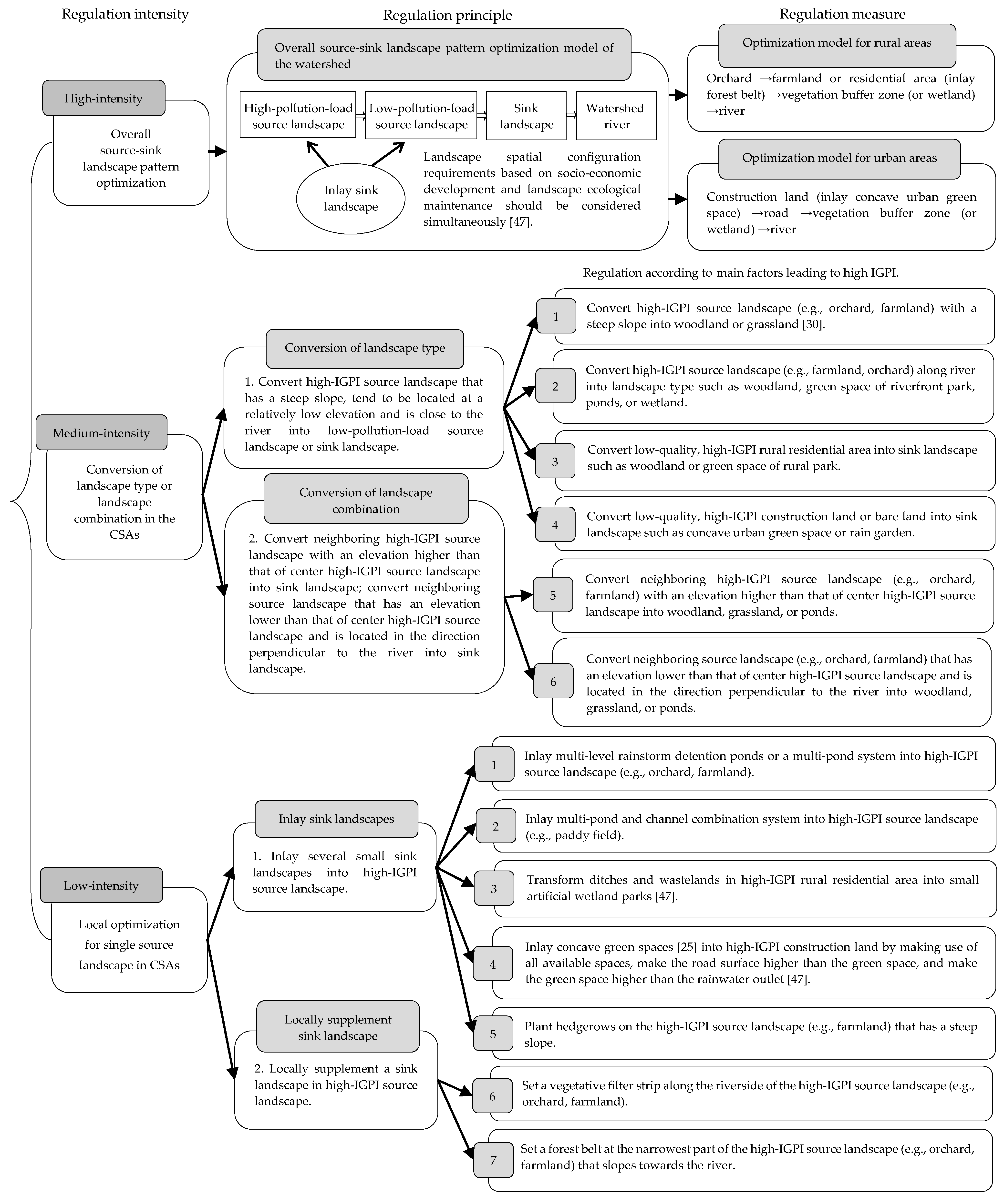
2.2. Comprehensive Regulation Strategy Formulation

2.2.1. Regulation Principles and Contents

Through the identification of CSAs, it is possible to regulate and optimize the overall landscape and the CSAs to promote the source-sink landscape to form a reasonable spatial distribution pattern in the watershed based on source-sink theory.

The landscape has multi-scale characteristics [54]. Additionally, as the scale and extent to which watershed landscape patterns can be adjusted are different, this study developed a comprehensive regulation strategy of CSAs from three landscape levels/regulation intensities to meet various regulatory intensity requirements of watershed areas, based on the landscape planning principle and a multi-scale landscape planning framework, as follows:

(1)

High-intensity regulation—overall source-sink landscape pattern optimization: based on the suitable positions of source and sink landscapes in terms of the distance from the river, relative elevation, and slope, an overall source-sink landscape pattern optimization model for the watershed was constructed and used as a macro regulation strategy of CSAs. Meanwhile, the requirements of watershed landscape spatial configuration based on socio-economic development and landscape ecological maintenance should be considered [47].

(2)

Medium-intensity regulation—conversion of landscape type or landscape combination in CSAs: at the meso-scale, as a reasonable combination of source and sink landscape can produce fewer NPS pollutants, high-IGPI source landscape can be converted into low-pollution-load source landscape or sink landscape, and for high-IGPI source landscape that is significantly affected by the neighboring landscapes, the neighboring source landscapes that significantly impact the aforementioned landscape can be transformed into sink landscape. Taking the above as the regulation principles, a series of corresponding regulation measures was formulated considering the landscape characteristics of urban and rural areas and the needs of socio-economic development. In actual regulation, appropriate regulation measures can be selected based on the main factors that lead to high IGPI.

(3)

Low-intensity regulation—local optimization for single source landscape in CSAs: at the micro-scale, for single high-IGPI source landscape in CSAs, several small sink landscapes can be inlayed [54] or a sink landscape can be locally supplemented in the high-IGPI source landscape without changing the type of source landscape. In light of the above regulation principles, a series of corresponding regulation measures was developed accordingly.

Generally, high-intensity regulation is suitable for watershed areas that the overall landscape spatial layout plan is not clear and can be adjusted at a large scale. Medium-intensity regulation is suitable for watershed areas that, the overall landscape spatial layout plan is clear; however, at the meso-scale and micro-scale, the landscape configuration scheme can still be adjusted. Low-intensity regulation is suitable for watershed areas that the landscape configuration scheme has been implemented and the adjustment of landscape type is relatively difficult. The decision maker can choose appropriate intensity regulation strategies for the watershed areas, to reduce the difficulty of implementation and reduce regulation costs, and finally improve the effectiveness of NPS pollution control in the watershed areas.

2.2.2. Formulation of Regulation Strategy

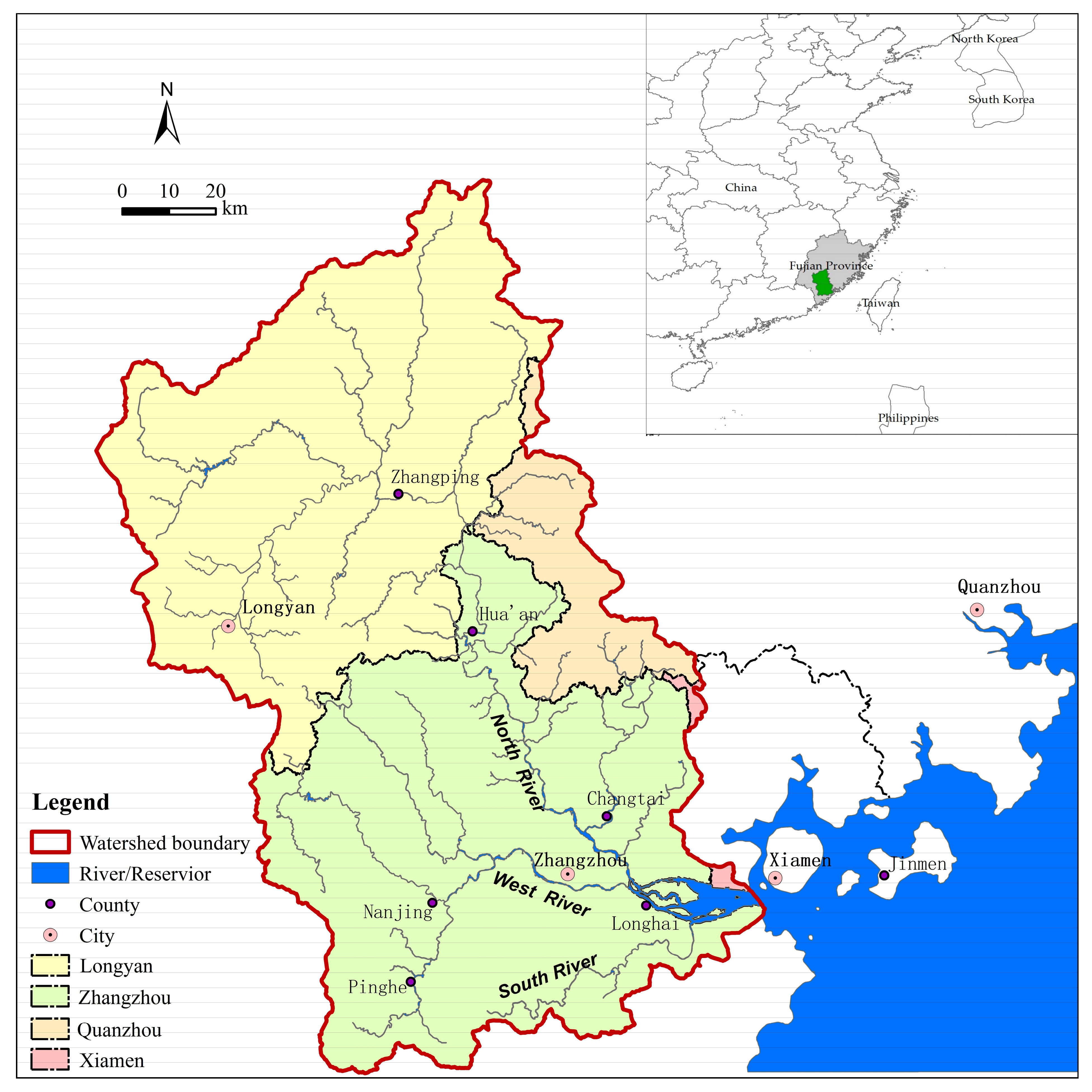
The comprehensive regulation strategy of CSAs of NPS pollution in the watershed is shown in Figure 1.

2.3. Study Area

The Jiulong River (116°46′55″–118°02′17″ E, 24°23′53″–25°53′38″ N) is the second-largest river in Fujian Province, China (Figure 2). North Stream originates in the Meihua Mountain area of Longyan City. West Stream originates in Banliao Ling in the western part of Nanjing County and Pinghe County. It flows through Zhangzhou Plain with a high level of agricultural intensification to Fugong Town, Longhai City, where the South Stream flows into it, and finally enters the sea through the port of Xiamen. The total length of the mainstream is 258 km, and the flow rate is 446 m³/s. The main soil types include red soil, lateritic red soil, and paddy soil. The watershed is located along the relatively economically developed southeastern coast of Fujian Province. It has a humid subtropical monsoon climate with a total area of 14,741 km², which accounts for about 12% of Fujian’s land area. It covers Longyan, Zhangzhou, Quanzhou, Xiamen, and other cities and encompasses 12 counties (cities, districts). In 2015, the watershed population was 6.53 million, accounting for 17% of the total population of Fujian Province, and the economic aggregate accounted for about 26.7% of Fujian Province. In recent years, rapid agricultural and population growths in the Jiulong River watershed and increasing NPS pollution in the watershed have led to significant water quality changes. Severe pollution of local bodies of water has affected the sustainable socio-economic development of the watershed.

2.4. Data Source and Processing

This study’s data mainly includes: (1) Land use data from remote sensing in 2015 (1:100,000), which was collected from the Resource and Environment Science and Data Center, Chinese Academy of Sciences (http://www.resdc.cn, accessed on 25 March 2018). We reclassified the land use data into nine categories according to the actual situation of the watershed and our research objectives: paddy field, dryland, woodland, orchard, grassland, water, construction land, rural area, and bare land (Figure 3). Most of the land in the watershed is woodland (58.31%), followed by grassland (15.27%), paddy field (8.69%), dryland (5.65%), orchard (4.50%), construction land (3.87%), and rural area (1.11%). (2) Digital elevation model (DEM) data: GDEM V2 was adopted, with a resolution of 30 m, derived from the Geospatial Data Cloud site, Computer Network Information Center, Chinese Academy of Sciences (http://www.gscloud.cn, accessed on 20 February 2018). (3) Water system and flow map, watershed socio-economic statistic data, and related development planning atlas. All of the spatial data were converted to Albers Equal Area Conic projection.

According to the landscape distribution characteristics of the watershed, the grid size of the study area was set as 300 m × 300 m. Supported by ArcGIS10.2 software, DEM data with a resolution of 30 m was aggregated into a 300 m digital elevation map, and the Slope command was used to form a slope map of the watershed. Based on the water system and landscape distribution data, the Euclidean Distance tool was applied to calculate the distance between each grid and the nearest river. Finally, the Fishnet and Identity tools were adopted based on the landscape distribution data to form a grid map in a unit size of 300 m × 300 m with landscape information.

2.5. Source-Sink Landscape Definition

For the definition of source-sink landscape of the study area, previous related research was defined mainly on the basis of expert’s knowledge [37,40,41,43]. For the determination of the NPS pollution weights of the source-sink landscapes, previous related research usually adopted methods such as field measurements [55], expert knowledge (especially for sink landscapes) [33,37], referring to the value of the cover-management factor (C) in the USLE [40] or estimation based on relevant literatures and materials [41,43,47].

In this study, the source landscape and sink landscape were defined based on the landscape characteristics of the Jiulong River watershed and by referring to the literature [37,40,43] (

Table 1. The source and sink landscape types of the Jiulong River watershed and the NPS pollution weights.

Source Landscape	Paddy Field	Dryland	Orchard	Construction Land	Rural Area	Bare Land
weight	0.90	0.80	1.00	0.28	0.42	0.21
Sink landscape	Woodland	Grassland
weight	−0.29	−0.22

Note: 1. As water is not the regulation subject but the protection objective, it is not defined in the table; 2. as the sink landscapes absorb pollutants, their weights are represented by negative values.

). To maintain the objectivity and accuracy of the determination of the NPS pollution weights of the source-sink landscapes, this study determined the NPS pollution weights of source-sink landscapes based on the discharge (for source landscape) and absorption (for sink landscape) of total nitrogen (TN) and total phosphorus (TP) per unit area of the landscapes. For the source landscapes, first, this study referred to a study regarding NPS pollution in the Jiulong River watershed [56] to obtain the discharge of TN and TP per unit area of the source landscapes in 2002. Second, to update the data for 2015, the correction coefficients of the TN and TP discharge per unit area of the source landscapes were computed. The change rates of the usage amounts of pesticides and fertilizers and the amounts of livestock and poultry in the watershed from 2002 to 2015 were computed (the amounts of rural domestic pollutants were not computed because of small changes) based on the Zhangzhou and Longyan Statistical Yearbooks (2002–2015). Then, according to the contribution ratios of pesticides and fertilizers, and livestock and poultry to the TN and TP of the Jiulong River watershed provided by [56], the correction coefficients were acquired. Finally, the discharge of TN and TP per unit area of the source landscapes in 2015 was obtained. For the sink landscapes, the absorption of TN and TP per unit area of woodland was computed based on [57,58] according to the woodland type and soil types of the Jiulong River watershed. Additionally, the absorption of TN and TP per unit area of grassland was estimated using the ratio of grassland to woodland (0.75) obtained from the literature [40]. On this basis, the NPS pollution weights of the landscapes were computed. As orchard has the largest discharge of TN and TP per unit area, it was assigned as the reference type; that is, the weight of orchard was set as 1, and the discharge of TN and TP per unit area of orchard was taken as the reference to compute the NPS pollution weights of other source landscapes and sink landscapes (Table 1).

3. Results

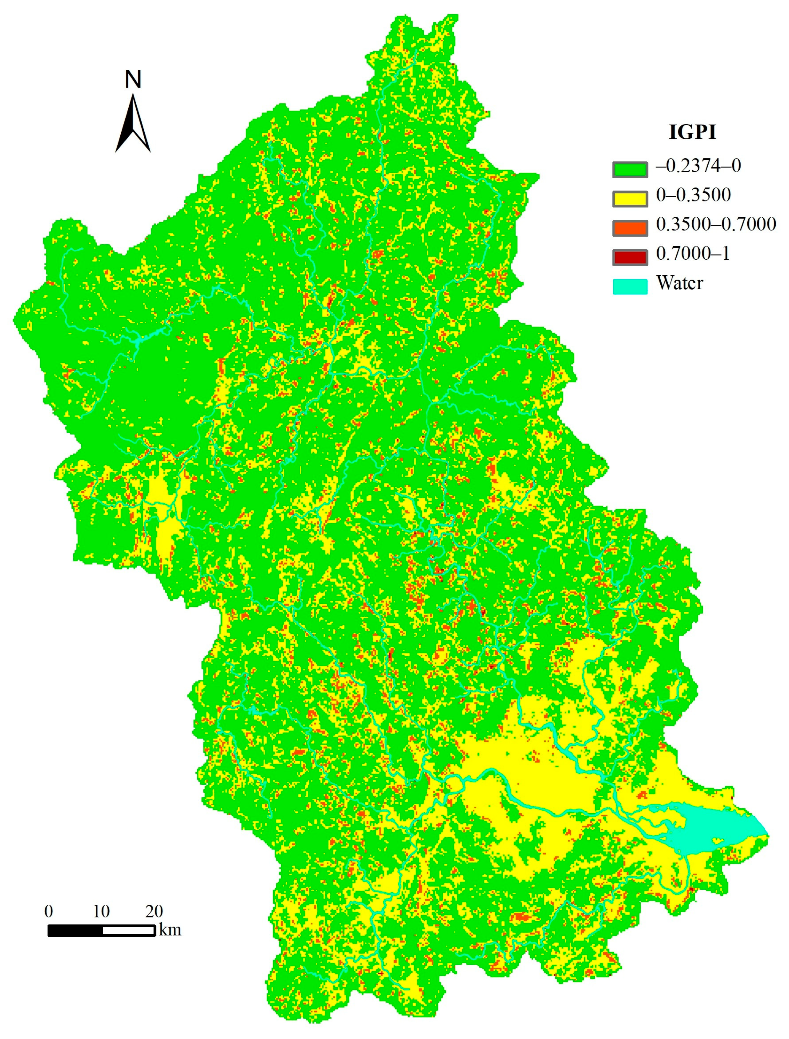
3.1. Identification Results of NPS Pollution CSAs

3.1.1. GLI, GPI, NII, and IGPI Calculations

The calculated GLI, GPI, NII_total, and IGPI are shown in Figure 4. As presented, GLI values range from (−0.2791)–1. Compared with Figure 3, the high-GLI areas are mainly concentrated in orchard landscape; this is because orchards have the largest discharge of NPS pollution per unit area, the weight is 1. When the entire grid is orchard landscape, the value of the GLI is maximum (value = 1). GPI values range from (−0.2407)–0.7821. Comparing the results of the GPI and GLI, we found that some high-value areas of GPI are consistent with GLI high-value areas. These areas not only have high GLI values but also have large slope, low elevation, and are close to the river, so the GPI values of these areas can still be high. However, in some high-GLI areas, due to the low slope, high elevation, and large distance from the river, their GPI values are no longer high. Examples include the large orchards in Longhai City and Xiangcheng District of Zhangzhou, the large paddy fields along the river in the southern part of Changtai County, Zhangzhou City, and the large paddy fields in the estuary of the Jiulong River. Hence, it can be seen that landscape slope, elevation, and distance from the river can affect the grid’s contribution to NPS pollution. As shown from the NII_total results, when the slope is relatively moderate, the value is small; the NII calculation formula can explain this. The final calculation of IGPI is between (−0.2374)–1 and the range is slightly larger than GPI due to the impacts of the neighboring grids on the center grid.

3.1.2. Identification of NPS Pollution CSAs

To identify the CSAs and facilitate watershed management, the IGPI values of the Jiulong River watershed were divided into four sections: (−0.2374)–0, 0–0.3500, 0.3500–0.7000, and 0.7000–1. When the value is less than 0, its GLI is negative, according to the GLI calculation formula; this can be defined as the sink action area. When the value is between 0–1, its GLI is positive and can be defined as the source action area, where 0.7000–1 is in a high-value section, defined as a source action high-pollution area; 0.3500–0.7000 is in a medium section, defined as source action medium-pollution area; and 0–0.3500 is in a low-value section, defined as source action low-pollution area. Source action high- and medium-pollution areas are the major contribution areas of NPS pollution in the watershed, that is, the CSAs of NPS pollution in the watershed. The area and percentage of NPS pollution CSAs and other areas in the Jiulong River watershed are listed in

Table 2. The area and percentage of NPS pollution CSAs in the Jiulong River watershed.

IGPI	Area Type		Area (km2)	Percentage (%)
(−0.2374)–0	–	Sink action area	10,060.74	67.93
0–0.3500	–	Source action low-pollution area	4091.94	27.63
0.3500–0.7000	CSAs	Source action medium-pollution area	648.27	4.38
0.7000–1	CSAs	Source action high-pollution area	8.64	0.06

, and the area and percentage of CSAs in the cities of the watershed are shown in

Table 3. The area and percentage of NPS pollution CSAs in the cities of the Jiulong River watershed.

City		Sink Action Area	Source Action Low-Pollution Area	CSAs
				Source Action Medium-Pollution Area	Source Action High-Pollution Area
Zhangzhou	Area (km2)	3904.11	2602.17	431.37	5.67
	Percentage (%)	56.23	37.48	6.21	0.08
Longyan	Area (km2)	5137.65	1242.9	183.33	1.35
	Percentage (%)	78.26	18.93	2.79	0.02
Xiamen	Area (km2)	41.67	24.3	1.53	0.27
	Percentage (%)	61.49	35.86	2.26	0.40
Quanzhou	Area (km2)	895.86	197.91	30.87	0.18
	Percentage (%)	79.64	17.59	2.74	0.02

.

Table 2 shows that the CSAs of NPS pollution covered 656.91 km², equivalent to 4.44% of the Jiulong River watershed. As shown in Figure 4 and Table 3, these CSAs were primarily distributed in Zhangzhou City and the southern of Zhangping City in the Longyan Region.

3.2. Regulation of NPS Pollution CSAs

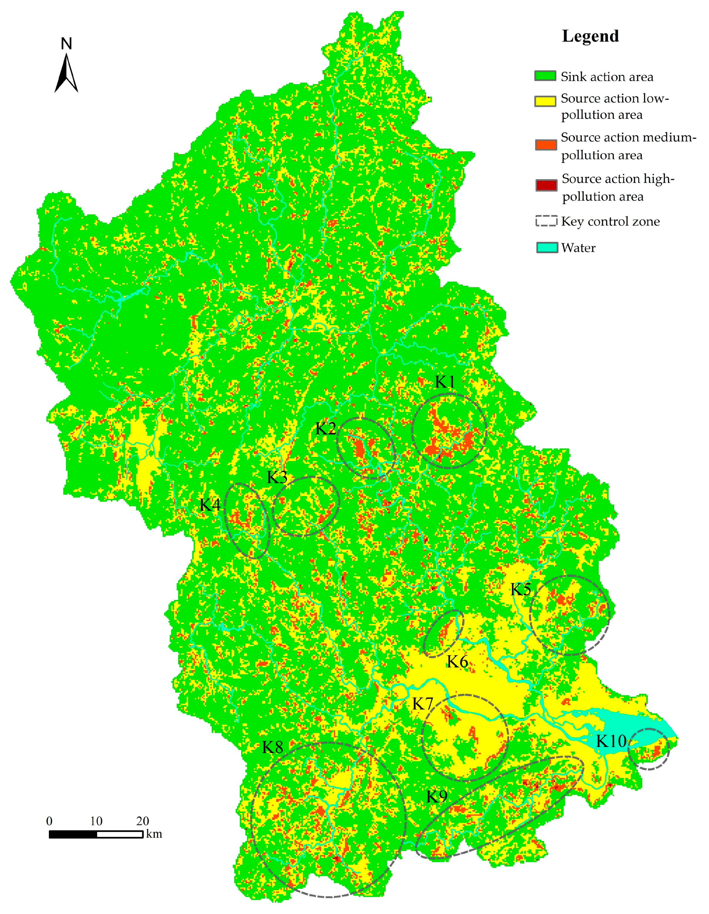
3.2.1. Division of Key Control Zones of CSAs

Based on Figure 4, Table 2 and Table 3, according to the IGPI spatial distribution status of CSAs, the regions that had spatially concentrated high value IGPI among the CSAs were identified to be the key control zones of CSAs. These areas were the key regulatory targets. They were divided into K1–K10, a total of 10 key control zones (Figure 5).

3.2.2. Regulation Strategies for Key Control Zones

Based on the method of the identification of NPS pollution CSAs, the reasons of the high pollution load in each key control zone were summarized. The GPI values of the following landscape types are high: the large orchard landscape with a steep slope, close to the river; the large paddy field landscape with a steep slope, a low elevation, and close to the river; and the large dryland landscape with a steep slope, close to the river. These landscape types all have high NPS pollution weights, so the GLI values are also high. After overlaying the actions of landscape slope, elevation, and distance from the river, the GPI values remain at a high level. Additionally, some landscapes also suffer from significant impacts of the neighboring landscapes, so their IGPI values still remain at a relatively high level. For these reasons, according to the regulation intensity requirements of the zones and the CSAs comprehensive regulation strategy (Figure 1), a series of medium- and low-intensity regulation measures was finally adopted to adjust and optimize the 10 key control zones. The regulation strategies adopted by the 10 key control zones are shown in

Table 4. The regulation strategies adopted by the 10 key control zones of the CSAs in the Jiulong River watershed.

High-IGPI Source Landscape	Regulation Intensity	Main Regulation Measures	Key Control Zone
Orchard landscape with a steep slope, close to the river	Medium intensity	1. Convert orchard with a steep slope into woodland or grassland.	K1, K2, K3, K4, K6, K7, K8, K9
		2. Convert orchard close to the river into woodland, ponds, or wetland.	K1, K2, K4, K5, K7, K8, K9
	Low intensity	1. Construction of multi-level rainstorm detention ponds in the orchard	K1, K2, K7, K8, K9
		2. Construction of a multi-pond system in the orchard	K1, K2, K7, K9, K10
		3. Set a forest belt (width 15–20 m) at the narrowest part of the orchard that slopes towards the river	K5, K6, K9
Orchard landscape affected by neighboring landscapes	Medium intensity	1. Convert neighboring high-IGPI source landscape (e.g., orchard, paddy field, dryland) with an elevation higher than that of center orchard landscape into woodland, grassland, or ponds	K2, K5, K6, K7, K9
		2. Convert neighboring source landscape (e.g., orchard, paddy field, dryland) that has an elevation lower than that of center orchard landscape and is located in the direction perpendicular to the river into woodland, grassland, or ponds	K1, K2, K7, K8, K10
Paddy field landscape with a steep slope, a low elevation and close to the river	Medium intensity	1. Convert paddy field with a steep slope along the river into landscape type such as woodland, ponds or wetland	K2, K4, K7, K9
	Low intensity	1. Build multi-pond and channel combination system in paddy field	K1, K2, K3, K5, K6, K7, K8, K9
		2. Set a vegetative filter strip (width 10–15 m) along the riverside of the paddy field	K2, K3, K8, K9
Dryland landscape with a steep slope and close to the river	Medium intensity	1. Convert dryland with a steep slope and close to the river into woodland or grassland	K2, K5, K6, K8, K9
	Low intensity	1. Build multi-level rainstorm detention ponds in the dryland with a steep slope	K4, K5, K7, K8, K9, K10
		2. Plant hedgerows in the dryland with a steep slope	K1, K2, K4, K5, K7, K8, K9
Rural residential area with a steep slope, a low elevation and close to the river	Low intensity	1. Transform ditches and wastelands in the rural residential area into small artificial wetland parks	K1, K5, K7, K8
Construction land with a steep slope, a low elevation and close to the river	Low intensity	1. Inlay concave green spaces into all available spaces in the construction land	K1, K4, K6, K7, K8

and Figure 6.

3.2.3. Prediction and Evaluation of Regulation Performance

To predict the regulation performance, this study recalculated the GLI, GPI, and IGPI of the watershed after regulation. The NPS pollution weights of the regulated landscapes were predetermined before recalculation. For the regulated landscape adopting medium-intensity regulation measures, the NPS pollution weight was predetermined according to the converted landscape type, and the NPS pollution weight of the new landscape type—wetland was determined as −0.19 by referring the ratio of wetland to woodland from the literature [55]. For the regulated landscape adopted low-intensity regulation measures, the correction coefficient of NPS pollution weight of the landscape was determined by referring to previous research or practices. The correction coefficient for orchard with the construction of multi-level rainstorm detention ponds or a multi-pond system was 0.35 [25,27,59]; that of paddy fields with the construction of multi-pond and channel combination systems was 0.30 [59]; that of paddy field with a vegetative filter strip (width 10–15 m) or orchard with a forest belt (width 15–20 m) was 0.50–0.45 [60,61,62]; that of dryland with the construction of multi-level rainstorm detention ponds was 0.30 [25,27]; that of dryland with the plant hedgerows was 0.50 [27]; and that of construction land with concave green spaces or rural area with small wetland parks was 0.50 [59,63]. When recalculating the GLI, the NPS pollution weight of the landscape adopting low-intensity regulation measures was the original weight multiplied by the correction coefficient. The IGPI prediction results of the watershed after regulation are shown in Figure 7.

According to the predicted values of the watershed IGPI after regulation, the areas of four numerical sections divided before regulation were recalculated. The area changes of CSAs in the Jiulong River watershed after regulation are listed in

Table 5. The area changes of NPS pollution CSAs after regulation in the Jiulong River watershed.

IGPI	Area Type		Area before Regulation (km2)	Percentage (%)	Area after Regulation (km2)	Percentage (%)	Area Change (km2)	Area Change Percentage (%)
(−0.2374)–0	–	Sink action area	10,060.74	67.93	10,182.06	68.75	121.32	1.21
0–0.3500	–	Source action low-pollution area	4091.94	27.63	4127.22	27.87	35.28	0.86
0.3500 −0.7000	CSAs	Source action medium-pollution area	648.27	4.38	493.65	3.33	−154.62	−23.85
0.7000–1	CSAs	Source action high-pollution area	8.64	0.06	6.66	0.04	−1.98	−22.92

Note: For area change, positive means increase; negative means decrease.

. The area changes of CSAs in the cities of the watershed after regulation are shown in

Table 6. The area changes of NPS pollution CSAs in the cities of the Jiulong River watershed after regulation.

City		Sink Action Area	Source Action Low-Pollution Area	CSAs
				Source Action Medium-Pollution Area	Source Action High-Pollution Area
Zhangzhou	Area change (km2)	108.09	29.25	−135.45	−1.89
	Percentage (%)	2.77	1.12	−31.40	−33.33
Longyan	Area change (km2)	13.59	5.76	−19.26	−0.09
	Percentage (%)	0.26	0.46	−10.51	−6.67
Xiamen	Area change (km2)	0	0	0	0
	Percentage (%)	0.00	0.00	0.00	0.00
Quanzhou	Area change (km2)	0	0.36	−0.36	0
	Percentage (%)	0.00	0.18	−1.17	0.00

Note: For area change, positive means increase; negative means decrease.

.

Comparing the IGPI before regulation (Figure 4) with the IGPI after regulation (Figure 7), it can be seen that the IGPIs in the regulated watershed are generally lower. After regulation, the area of sink action areas in entire watershed was predicted to increase by 1.21%, whereas the area of source action medium-pollution areas was predicted to decrease by 23.85% (Table 5 and Table 6), and the area of source action high-pollution areas was predicted to decrease by 22.92%. The CSAs of NPS pollution were predicted to be totally reduced by 23.84%. After regulation, the CSAs in Zhangzhou City, Longyan City, and Quanzhou City were predicted to be reduced by 31.43%, 10.48%, and 1.16%, respectively. Due to the small CSAs in Xiamen City, it was not included in the key control zone for regulation, thus the area remains unchanged.

Therefore, after taking a series of medium- and low-intensity regulation measures for the key control zones of CSAs, the CSAs of the Jiulong River watershed were predicted to be significantly reduced, and the sink action areas were predicted to increase. The impacts on the water environment quality of the watershed were predicted to be reduced. Some of the CSAs in the Jiulong River watershed are relatively spatially concentrated while others are relatively scattered, and this research mainly took the relatively concentrated areas as the key control zones for regulation. Therefore, the prediction results only reflected the regulation effect of relatively concentrated CSAs. If the scattered CSAs are regulated simultaneously, the predicted effect of regulation will be more significant.

4. Discussion

4.1. Advantages and Applicability of the CSAs Identification Model

Source-sink theory provides a new approach for the identification of NPS pollution CSAs in watersheds. After the case study, we compared the proposed CSAs identification model with other CSAs identification related models used or proposed in previous studies (

Table 7. A comparison of the proposed CSAs identification model with those used or proposed in previous studies.

Model		Requirement	Research Unit	Applicable Watershed
Traditional model	AnnAGNPS, SWAT, HSPF, USLE *	Hydrology, soil, land use/cover, meteorology, and water quality data; a large number of parameters [21,22]; complex operation process [19,22]	Sub-watershed, hydrological response units or grid	Watersheds of all scales
Source-sink theory-based model	Location-weighted landscape contrast index (LCI) [30], location-weighted landscape index (LWLI) [37]	The data of landscape type, area, spatial location, distance from river, relative elevation, and slope	Watershed, sub-watershed	Large watersheds
	Precipitation-weighted landscape structure model (LSM) [19], source precipitation landscape model (SPLM) [42]	The data of precipitation, landscape structure and pollution sources	Sub-watershed	Large watersheds
	Grid-based LCI [43]	The data of landscape type, area, spatial location, distance from river, relative elevation, and slope	Grid	Small watersheds
	CSAs identification model in this study	The data of landscape type, area, spatial distribution, slope, relative elevation, and distance from river	Grid, including neighborhood impact analysis	Medium and small watersheds

* Annualized AGricultural Non-Point Source pollution (AnnAGNPS), Soil and Water Assessment Tool (SWAT), Hydrological Simulation Program-FORTRAN (HSPF), and the Universal Soil Loss Equation (USLE).

). The results show that, in general, methods based on source-sink theory have the advantages of easy data access, a simple operation process and convenient implementation for regulation, and avoid the problems of large data demand [18,19,20], large numbers of parameters [21,22], and complex operation [19,22] in the traditional models. The LCI/LWLI and the LSM/SPLM models are constructed with the sub-watershed as the research unit, which are suitable for large watersheds. However, for medium and small watersheds, the accuracy of identification with the sub-watershed as the research unit is insufficient for CSAs assessment and regulation. Using the grid as the research unit is more accurate than using the sub-watershed. However, the impacts of the surrounding landscapes on the central grid’s NPS pollution discharge have not been considered in previous grid-based studies. By using the Moore neighborhood analysis method, this study constructed a neighborhood impact index (NII) to calculate the impacts from the surrounding landscape grids on the central grid’s output of NPS pollution, which made the grid-based research more scientific in the evaluation of the rationality of the source-sink landscape pattern and overcame the limitation of previous grid-based research.

4.2. Advantages and Significance of the Comprehensive CSAs Regulation Strategy

At present, NPS pollution control in watersheds is mainly based on the implementation of BMPs. As landscape pattern significantly affecting the NPS pollution in the watershed has been a recognized fact [29,32,34,35,36], this study considers the watershed NPS pollution control at a larger scale. Based on the principle that a reasonable source-sink landscape spatial distribution pattern can produce fewer NPS pollutants [31], and a multi-scale landscape planning framework, a comprehensive regulation strategy for NPS pollution CSAs was developed, which includes overall source-sink landscape pattern optimization at the macro-scale, conversion of landscape type or landscape combination in CSAs at the meso-scale, and local optimization for single source landscape in CSAs at the micro-scale. The comprehensive regulation framework avoided the problems of the BMPs, such as the lack of system control [28], and remaining at the technical level of problem-specific analysis [27], which lead to an unstable governance effect [27,28]. It was shown to be relatively comprehensive, systematic, and effective. In addition, the three scales of regulation correspond to three regulation intensities. The CSAs regulation strategies can be formulated according to the regulation intensity requirements of the area, thus ensuring the effective implementation of CSAs regulation strategy based on the land use demands of local social and economic development, decreasing regulation costs, and improving the effectiveness of NPS pollution control. Previous studies on the landscape pattern regulation for watershed NPS pollution control based on source-sink theory still remain at the stage of theoretical exploration and preliminary framework construction [28,31,46,47,48,49]. This study provides a relatively concrete and operational regulation framework.

4.3. Implications for Watershed Management

The new methodological framework for the identification and regulation of NPS pollution CSAs proposed in this study can provide strong technical support to governments to improve the effectiveness of watershed management. Firstly, the CSAs identification model can quickly and effectively identify the CSAs with easy data access and simple operation. Additionally, the identifying results are convenient for CSAs management and regulation as they can show the specific high-pollution-load source landscapes in the CSAs, which are better than the results obtained when using the sub-watershed as the research unit. Secondly, the proposed comprehensive CSAs regulation strategy based on source-sink theory is cost-effective since it does not require considerable contamination treatment costs. Furthermore, as watershed areas are often in different stages of development and construction, the regulation scale and extent of the landscape pattern are different. In some watershed areas, the overall landscape plan is not clear and can be adjusted at a large scale; in others, the overall landscape plan is clear, however, the landscape configuration scheme can still be adjusted; and in others, a landscape configuration scheme has been implemented and the adjustment of landscape type is relatively difficult. The proposed CSAs regulation framework can provide different intensity regulation strategies for the different watershed areas, which can help decision makers to choose the appropriate strategies to reduce the difficulty of implementation and the regulation costs, simultaneously ensure the land use demands of local social and economic development, and finally improve the effectiveness of NPS pollution control and promote the coordinated development of the social economy and the environment.

4.4. Limitations of the Study and Future Research

However, there are some limitations of this study. The proposed identification model for the NPS pollution CSAs is suitable for medium or small watersheds with simplex soil and precipitation conditions, as the effects of diverse soil and precipitation conditions are not considered in the model. Moreover, the model validation is also a limitation of this study. In addition, as the scale of this study is relatively large, the design scheme of the low-intensity regulation measures for the key control zones of the CSAs in the case study shall be further refined in the implementation based on the characteristics of the specific location. Furthermore, when predicting the IGPIs after regulation, this study set correction coefficients for the NPS pollution weights of the regulated source landscapes adopting low-intensity regulation measures. As the correction coefficients were set by referring to the values of 75–80% of the pollutant removal rates reported in the literatures, the actual regulation effects may be better than the predicted effects. Finally, the macro-regulation strategy—namely, overall source-sink landscape pattern optimization—was not adopted in the case study as the land use planning of the Jiulong River watershed had already been carried out and would be hard to change in a short time. Supposing that the macro-regulation strategy for the watershed is considered during the process of the watershed land use planning, the NPS pollution regulation of the watershed’s CSAs will be the most effective.

In the future research, we plan to improve the CSAs identification model by taking into account diverse soil and precipitation conditions of the watershed, so that the model can be applied to larger watersheds. Additionally, we will also improve the medium- and low-intensity regulation measures of the comprehensive CSAs regulation strategy through more case studies, simultaneously by incorporating low impact development (LID) techniques into the regulation measures to make the regulation strategy more suitable for high urbanization watersheds.

5. Conclusions

This study systematically developed a new methodological framework for the identification and regulation of NPS pollution CSAs in medium and small watersheds based on source-sink theory. A grid-based CSAs quantitative identification model was proposed that involved the evaluation of the rationality of the source-sink landscape pattern and three main geographical factors (landscape slope, relative elevation, and the distance from the river) and identified CSAs by calculating IGPI. Based on a multi-scale landscape planning framework, a comprehensive CSAs regulation strategy aiming to meet various regulatory requirements of the watershed areas was developed from three landscape levels/regulation intensities: (1) High-intensity regulation: overall source-sink landscape pattern optimization. As the macro-regulation strategy of CSAs, a model for the optimization of the watershed’s overall source-sink landscape pattern was constructed at the macro-scale; (2) medium-intensity regulation: conversion of landscape type or landscape combination in CSAs. At the meso-scale, based on the principle that a reasonable combination of source and sink landscapes can produce fewer NPS pollutants, regulation guidelines and specific regulation measures were formulated for the high-IGPI source landscape and the neighboring source landscape that have significant impacts on the central high-IGPI source landscape; and (3) low-intensity regulation: local optimization for single source landscape in CSAs. At the micro-scale, for single source landscape in CSAs, based on the regulation principle that several small sink landscapes can be inlayed or a small sink landscape can be locally supplemented in the source landscape, specific regulation measures were formulated.

The established methodological framework was applied to the Jiulong River watershed in Fujian Province, China. The identified CSAs mainly included orchard, paddy field and dryland landscape that had a steep slope, low elevation, were close to the river, and were affected by neighboring landscapes. Multiple-intensity regulation measures were adopted to 10 key control zones among the CSAs. The watershed IGPIs were predicted to be generally reduced and the area of CSAs was predicted to decrease following the proposed regulations.

The results of case study and the comparison with previous study indicate that, the proposed CSAs identification model can identify the CSAs with easy data access and simple operation. And, the identifying results are convenient for the CSAs management and regulation. The utilization of neighborhood impact analysis in the model makes the grid-based research more scientific in the evaluation of the rationality of the source-sink landscape pattern. The application of multi-scale landscape planning framework and the principle of source-sink landscape pattern regulation make the CSAs regulation strategy systematic and cost-effective, compared with BMPs and previous research. And, the provision of different intensity regulation strategies makes the regulation strategy easy to implement and relatively low cost, and simultaneously ensures local social and economic development.

The proposed new methodological framework can provide technical support for governments in medium and small watershed areas to quickly and accurately identify the NPS pollution CSAs, and systematically and effectively control the NPS pollution of the watershed.

References

1. Xue, L.; Hou, P.; Zhang, Z.; Shen, M.; Liu, F.; Yang, L. Application of systematic strategy for agricultural non-point source pollution control in Yangtze River basin, China. Agric. Ecosyst. Environ. 2020, 304, 107148. [Google Scholar] [CrossRef]
2. Liu, R.; Xu, F.; Zhang, P.; Yu, W.; Men, C. Identifying non-point source critical source areas based on multi-factors at a basin scale with SWAT. J. Hydrol. 2016, 533, 379–388. [Google Scholar] [CrossRef]
3. Zou, L.; Liu, Y.; Wang, Y.; Hu, X. Assessment and analysis of agricultural non-point source pollution loads in China: 1978–2017. J. Environ. Manag. 2020, 263, 110400. [Google Scholar] [CrossRef]
4. Marsh, W.M. Landscape Planning: Environmental Applications; John Wiley & Sons: New York, NY, USA, 2005. [Google Scholar]
5. Gao, C.; Zhu, J.; Zhu, J.; Gao, X.; Dou, Y.; Hosen, Y. Nitrogen export from an agriculture watershed in the Taihu Lake area, China. Environ. Geochem. Health 2004, 26, 199–207. [Google Scholar] [CrossRef] [PubMed]
6. Gburek, W.J.; Sharpley, A.N. Hydrologic Controls on Phosphorus Loss from Upland Agricultural Watersheds. J. Environ. Qual. 1998, 27, 267–277. [Google Scholar] [CrossRef]
7. Shore, M.; Jordan, P.; Mellander, P.-E.; Kelly-Quinn, M.; Wall, D.; Murphy, P.; Melland, A. Evaluating the critical source area concept of phosphorus loss from soils to water-bodies in agricultural catchments. Sci. Total Environ. 2014, 490, 405–415. [Google Scholar] [CrossRef] [PubMed]
8. Uribe, N.; Srinivasan, R.; Corzo, G.; Arango, D.; Solomatine, D. Spatio-temporal critical source area patterns of runoff pollution from agricultural practices in the Colombian Andes. Ecol. Eng. 2020, 149, 105810. [Google Scholar] [CrossRef]
9. Rudra, R.; Mekonnen, B.; Shukla, R.; Shrestha, N.; Goel, P.; Daggupati, P.; Biswas, A. Currents Status, Challenges, and Future Directions in Identifying Critical Source Areas for Non-Point Source Pollution in Canadian Conditions. Agriculture 2020, 10, 468. [Google Scholar] [CrossRef]
10. Huang, J.J.; Lin, X.; Wang, J.; Wang, H. The precipitation driven correlation based mapping method (PCM) for identifying the critical source areas of non-point source pollution. J. Hydrol. 2015, 524, 100–110. [Google Scholar] [CrossRef]
11. Pérez-Gutiérrez, J.D.; Paz, J.O.; Tagert, M.L.M.; Yasarer, L.M.W.; Bingner, R.L. Using AnnAGNPS to Simulate Runoff, Nutrient, and Sediment Loads in an Agricultural Catchment with an On-Farm Water Storage System. Climate 2020, 8, 133. [Google Scholar] [CrossRef]
12. Zhu, Q.; Sun, J.; Hua, G.; Wang, J.; Wang, H. Runoff characteristics and non-point source pollution analysis in the Taihu Lake Basin: A case study of the town of Xueyan, China. Environ. Sci. Pollut. Res. 2015, 22, 15029–15036. [Google Scholar] [CrossRef] [PubMed]
13. Tan, M.L.; Gassman, P.W.; Srinivasan, R.; Arnold, J.G.; Yang, X. A Review of SWAT Studies in Southeast Asia: Applications, Challenges and Future Directions. Water 2019, 11, 914. [Google Scholar] [CrossRef] [Green Version]
14. Jeon, J.-H.; Yoon, C.G.; Donigian, A.S.; Jung, K.-W. Development of the HSPF-Paddy model to estimate watershed pollutant loads in paddy farming regions. Agric. Water Manag. 2007, 90, 75–86. [Google Scholar] [CrossRef]
15. Chen, Y.; Xu, C.-Y.; Chen, X.; Xu, Y.; Yin, Y.; Gao, L.; Liu, M. Uncertainty in simulation of land-use change impacts on catchment runoff with multi-timescales based on the comparison of the HSPF and SWAT models. J. Hydrol. 2019, 573, 486–500. [Google Scholar] [CrossRef]
16. Wu, L.; Liu, X.; Ma, X.-Y. Spatio-temporal variation of erosion-type non-point source pollution in a small watershed of hilly and gully region, Chinese Loess Plateau. Environ. Sci. Pollut. Res. 2016, 23, 10957–10967. [Google Scholar] [CrossRef]
17. Alewell, C.; Borrelli, P.; Meusburger, K.; Panagos, P. Using the USLE: Chances, challenges and limitations of soil erosion modelling. Int. Soil Water Conserv. Res. 2019, 7, 203–225. [Google Scholar] [CrossRef]
18. Zhang, H.; Huang, G. Assessment of non-point source pollution using a spatial multicriteria analysis approach. Ecol. Model. 2011, 222, 313–321. [Google Scholar] [CrossRef]
19. Sun, R.; Cheng, X.; Chen, L. A precipitation-weighted landscape structure model to predict potential pollution contributions at watershed scales. Landsc. Ecol. 2018, 33, 1603–1616. [Google Scholar] [CrossRef]
20. Matias, N.-G.; Johnes, P.J. Catchment Phosphorous Losses: An Export Coefficient Modelling Approach with Scenario Analysis for Water Management. Water Resour. Manag. 2011, 26, 1041–1064. [Google Scholar] [CrossRef]
21. Yan, X.; Lu, W.; An, Y.; Dong, W. Assessment of parameter uncertainty for non-point source pollution mechanism modelling: A Bayesian-based approach. Environ. Pollut. 2020, 263, 114570. [Google Scholar] [CrossRef]
22. Cheng, X.; Chen, L.; Sun, R.; Jing, Y. An improved export coefficient model to estimate non-point source phosphorus pollution risks under complex precipitation and terrain conditions. Environ. Sci. Pollut. Res. 2018, 25, 20946–20955. [Google Scholar] [CrossRef]
23. Lei, N.; Huang, D. Research on risk assessment of agricultural non-point source pollution with GIS. Chin. Agric. Sci. Bull. 2007, 23, 381–385. [Google Scholar]
24. United State Environmental Protection Agency. National Management Measures to Control non Point Source Pollution from Urban Area; United State Environmental Protection Agency: Washington, DC, USA, 2005.
25. Liu, Y.; Engel, B.A.; Flanagan, D.C.; Gitau, M.W.; McMillan, S.K.; Chaubey, I. A review on effectiveness of best management practices in improving hydrology and water quality: Needs and opportunities. Sci. Total Environ. 2017, 601–602, 580–593. [Google Scholar] [CrossRef] [PubMed]
26. Liu, G.; Chen, L.; Wei, G.; Shen, Z. New framework for optimizing best management practices at multiple scales. J. Hydrol. 2019, 578, 124133. [Google Scholar] [CrossRef]
27. Sun, Q.; Zhang, C.; Yu, X.; Li, J.; Zhang, Y.; Gao, Y. Best management practices of agricultural non-point source pollution in China: A review. Chin. J. Ecol. 2013, 32, 772–778. [Google Scholar] [CrossRef]
28. Diebel, M.W.; Maxted, J.T.; Nowak, P.J.; Zanden, J.V. Landscape Planning for Agricultural Nonpoint Source Pollution Reduction I: A Geographical Allocation Framework. Environ. Manag. 2008, 42, 789–802. [Google Scholar] [CrossRef]
29. Flynn, K.M.; Lockaby, B.G. Relationships Between Landscape Characteristics and Nonpoint Source Pollution Inputs to Coastal Estuaries. Environ. Manag. 1999, 23, 539–549. [Google Scholar] [CrossRef]
30. Chen, L.; Fu, B.; Xu, J.; Gong, J. Location-weighted landscape contrast index: A scale independent approach for landscape pattern evaluation based on “Source-Sink” ecological processes. Acta Ecol. Sin. 2003, 23, 2407–2413. [Google Scholar]
31. Chen, L.; Fu, B.; Zhao, W. Source-sink landscape theory and its ecological significance. Front. Biol. China 2008, 3, 131–136. [Google Scholar] [CrossRef]
32. Lee, S.-W.; Hwang, S.-J.; Lee, S.-B.; Hwang, H.-S.; Sung, H.-C. Landscape ecological approach to the relationships of land use patterns in watersheds to water quality characteristics. Landsc. Urban Plan. 2009, 92, 80–89. [Google Scholar] [CrossRef]
33. Wang, J.; Ni, J.; Chen, C.; Xie, D.; Shao, J.; Chen, F.; Lei, P. Source-sink landscape spatial characteristics and effect on non-point source pollution in a small catchment of the Three Gorge Reservoir Region. J. Mt. Sci. 2018, 15, 327–339. [Google Scholar] [CrossRef]
34. Wu, J.; Lu, J. Landscape patterns regulate non-point source nutrient pollution in an agricultural watershed. Sci. Total Environ. 2019, 669, 377–388. [Google Scholar] [CrossRef]
35. Zhang, Y.; Bi, Z.; Zhang, X.; Yu, Y. Influence of Landscape Pattern Changes on Runoff and Sediment in the Dali River Watershed on the Loess Plateau of China. Land 2019, 8, 180. [Google Scholar] [CrossRef] [Green Version]
36. Song, Y.; Song, X.; Shao, G. Response of Water Quality to Landscape Patterns in an Urbanized Watershed in Hangzhou, China. Sustainability 2020, 12, 5500. [Google Scholar] [CrossRef]
37. Chen, L.; Tian, H.; Fu, B.; Zhao, X. Development of a new index for integrating landscape patterns with ecological processes at watershed scale. Chin. Geogr. Sci. 2009, 19, 37–45. [Google Scholar] [CrossRef] [Green Version]
38. Wang, J.; Chen, C.; Ni, J.; Xi, G.; Guo, X.; Luo, Z.; Zhao, Y. Assessing effects of “source-sink” landscape on non-point source pollution based on cell units of a small agricultural catchment. J. Mt. Sci. 2019, 16, 2048–2062. [Google Scholar] [CrossRef]
39. Wu, Z.; Lin, C.; Su, Z.; Zhou, S.; Zhou, H. Multiple landscape “source–sink” structures for the monitoring and management of non-point source organic carbon loss in a peri-urban watershed. Catena 2016, 145, 15–29. [Google Scholar] [CrossRef]
40. Sun, R.; Chen, L.; Wang, W.; Wang, Z. Correlating landscape pattern with total nitrogen concentration using a location-weighted sink-source landscape index in the Haihe River Basin, China. Environ. Sci. 2012, 33, 1784–1788. [Google Scholar]
41. Xu, F.; Zhou, X.; Meng, Q.; Zhang, Y. Remote sensing identification and evaluation of non-point source pollution risk of drinking water source based on “source-sink” landscape. Acta Ecol. Sin. 2020, 40, 2609–2620. [Google Scholar] [CrossRef]
42. Cheng, X.; Chen, L.; Sun, R. Modeling the non-point source pollution risks by combing pollutant sources, precipitation, and landscape structure. Environ. Sci. Pollut. Res. 2019, 26, 11856–11863. [Google Scholar] [CrossRef] [PubMed]
43. Jiang, M.; Chen, H.; Chen, Q. A method to analyze “source–sink” structure of non-point source pollution based on remote sensing technology. Environ. Pollut. 2013, 182, 135–140. [Google Scholar] [CrossRef]
44. Wang, J.; Shao, J.; Wang, D.; Ni, J.; Xie, D. Identification of the “source” and “sink” patterns influencing non-point source pollution in the Three Gorges Reservoir Area. J. Geogr. Sci. 2016, 26, 1431–1448. [Google Scholar] [CrossRef]
45. Zhu, K.; Chen, Y.; Zhang, S.; Yang, Z.; Huang, L.; Lei, B.; Li, L.; Zhou, Z.; Xiong, H.; Li, X. Identification and prevention of agricultural non-point source pollution risk based on the minimum cumulative resistance model. Glob. Ecol. Conserv. 2020, 23, e01149. [Google Scholar] [CrossRef]
46. Yue, J.; Wang, Y.; Li, G.; Wu, J. The conceptual framework of watershed landscape optimization concerning water environmental protection. Prog. Geogr. 2007, 26, 38–46. [Google Scholar]
47. Huang, N.; Wang, H.; Lin, T.; Liu, Q.; Huang, Y.; Li, J. Regulation framework of watershed landscape pattern for non-point source pollution control based on ’source-sink’ theory: A case study in the watershed of Maluan Bay, Xiamen City, China. Chin. J. Appl. Ecol. 2016, 27, 3325–3334. [Google Scholar]
48. Lin, L.; Li, M.; Chen, H.; Lai, X.; Zhu, H.; Wang, H. Integrating landscape planning and stream quality management in mountainous watersheds: A targeted ecological planning approach for the characteristic landscapes. Ecol. Indic. 2020, 117, 106557. [Google Scholar] [CrossRef]
49. Maxted, J.T.; Diebel, M.W.; Zanden, J.V. Landscape Planning for Agricultural Nonpoint Source Pollution Reduction. II. Balancing Watershed Size, Number of Watersheds, and Implementation Effort. Environ. Manag. 2008, 43, 60–68. [Google Scholar] [CrossRef] [PubMed] [Green Version]
50. Jiang, M.; Chen, H.; Chen, Q.; Wu, H. Study of landscape patterns of variation and optimization based on non-point source pollution control in an estuary. Mar. Pollut. Bull. 2014, 87, 88–97. [Google Scholar] [CrossRef]
51. Tian, Y.; Huang, Z.; Xiao, W. Reductions in non-point source pollution through different management practices for an agricultural watershed in the Three Gorges Reservoir Area. J. Environ. Sci. 2010, 22, 184–191. [Google Scholar] [CrossRef]
52. Zhang, T.; Yang, Y.; Ni, J.; Xie, D. Construction of an integrated technology system for control agricultural non-point source pollution in the Three Gorges Reservoir Areas. Agric. Ecosyst. Environ. 2020, 295, 106919. [Google Scholar] [CrossRef]
53. Campos, P.B.R.; de Almeida, C.M.; de Queiroz, A.P. Educational infrastructure and its impact on urban land use change in a peri-urban area: A cellular-automata based approach. Land Use Policy 2018, 79, 774–788. [Google Scholar] [CrossRef]
54. Forman, R.T.T.; Godron, M. Landscape Ecology; John Wiley & Sons: New York, NY, USA, 1986. [Google Scholar]
55. Wang, Y.; Zhang, J.; Chen, G.; Xu, Y.; Chen, Y.; Liu, Y. Spatiotemporal characteristics of water quality in Taihu Lake watershed based on ’source-sink’ landscape change. Chin. J. Ecol. 2012, 31, 399–405. [Google Scholar]
56. Huang, J.; Hong, H.; Zhang, L.; Du, P. Nitrogen and phosphorus loading of agricultural non-point sources in Jiulong River watershed based on GIS. J. Agro-Environ. Sci. 2004, 23, 866–871. [Google Scholar]
57. Zhan, S.; Chen, F.; Hu, X.; Gan, L.; Zhu, Y. Soil nitrogen and phosphorus availability in forest ecosystems at different stages of succession in the central subtropical region. Acta Ecol. Sin. 2009, 29, 4673–4680. [Google Scholar]
58. Liu, Q.; Cao, Y.; Huang, Y.; Zhang, Y.; Lin, J.; Lin, J.; Xu, L. Soil organic matter dynamics after C3–C4 vegetation change of red soil in Southern, China: Evidence from natural 13C abundance. Contemp. Probl. Ecol. 2013, 6, 513–519. [Google Scholar] [CrossRef]
59. Chen, H. Surface-Flow Constructed Treatment Wetlands for Pollutant Removal: Applications and Perspectives. Wetlands 2011, 31, 805–814. [Google Scholar] [CrossRef]
60. Shin, J.; Gil, K. Effect of rainfall characteristics on removal efficiency evaluation in vegetative filter strips. Environ. Earth Sci. 2013, 72, 601–607. [Google Scholar] [CrossRef]
61. Shin, J.; Gil, K. Determination of removal efficiency using vegetative filter strips based on various efficiency evaluation methods. Environ. Earth Sci. 2014, 73, 6437–6444. [Google Scholar] [CrossRef]
62. Gao, J.; You, Y.; Tan, X.; Miao, Z. The mechanism and research progress of runoff pollution control by vegetative filter strips. Environ. Sci. Technol. 2019, 42, 91–97. [Google Scholar] [CrossRef]
63. Du, S.; Wang, C.; Shen, J.; Wen, J.; Gao, J.; Wu, J.; Lin, W.; Xu, H. Mapping the capacity of concave green land in mitigating urban pluvial floods and its beneficiaries. Sustain. Cities Soc. 2019, 44, 774–782. [Google Scholar] [CrossRef]
Figure 1. The comprehensive regulation system of CSAs of NPS pollution in watershed based on source-sink theory [25,30,47].
Land 10 00668 g001
Figure 2. Basic geographical information of the Jiulong River watershed.
Land 10 00668 g002
Figure 3. Landscape distribution of the Jiulong River watershed in 2015.
Land 10 00668 g003
Figure 4. The results of NPS pollution CSAs identification calculation in the Jiulong River watershed.
Land 10 00668 g004
Figure 5. The key control zones of NPS pollution CSAs in the Jiulong River watershed.
Land 10 00668 g005
Figure 6. The medium- and low-intensity regulation strategies for the 10 key control zones in the Jiulong River watershed.
Land 10 00668 g006
Figure 7. The prediction results of IGPI after regulation of the Jiulong River watershed.
Land 10 00668 g007