Article

Linking Ecosystem Service Supply–Demand Risks and Regional Spatial Management in the Yihe River Basin, Central China

1
College of Resources and Environmental Sciences, Henan Agricultural University, Zhengzhou 450002, China
2
Henan Engineering Research Center of Land Consolidation and Ecological Restoration, Henan Agricultural University, Zhengzhou 450002, China
3
Faculty of Geographical Science, Beijing Normal University, Beijing 100875, China
*
Author to whom correspondence should be addressed.
The two authors contributed equally to this work.
Land 2021, 10(8), 843; https://doi.org/10.3390/land10080843
Submission received: 2 June 2021 / Revised: 1 August 2021 / Accepted: 10 August 2021 / Published: 11 August 2021

Abstract

:
The continuous supply of ecosystem services is the foundation of the sustainable development of human society. The identification of the supply–demand relationships and risks of ecosystem services is of considerable importance to the management of regional ecosystems and the effective allocation of resources. This paper took the Yihe River Basin as the research area and selected water yield, carbon sequestration, food production, and soil conservation to assess changes in the supply and demand of ecosystem services and their matching status from 2000 to 2018. Risk identification and management zoning were also conducted. Results show the following: (1) The spatial distribution of the four ecosystems service supply and demand in the Yihe River Basin was mismatched. The food production supply levels in the middle and lower reaches and the upstream water yield, carbon sequestration, and soil conservation supply levels were high. However, most of the areas with high demand for ecosystem services were concentrated downstream. (2) From 2000 to 2018, the supply of water yield and carbon sequestration in the Yihe River Basin decreased, while that of food production and soil conservation increased. The demand for the four ecosystem services also increased. (3) Water yield faced considerable supply–demand risks. Fifty percent of the sub-basins were at a high-risk level, and the risk areas were concentrated in the middle and lower reaches. The three remaining services were mainly at low-risk levels. The Yihe River Basin was divided into eight types of supply–demand risk spatial management zones based on the ecosystem service supply and demand levels, which will help promote refined regional ecosystem management and sustainable development. The supply and demand assessment of ecosystem services from a risk perspective can integrate the information of natural ecosystems and socio-economic systems and provide scientific support for watershed spatial management.

1. Introduction

Ecosystem services refer to the natural resources and commodities comprising natural ecosystems [1,2,3], which can be directly used or consumed by humans, and maintain the environmental conditions for human survival and development [4,5]. These services are the resource and environmental basis for human survival and development. For a long time, people’s lack of understanding of the importance of ecosystem services has caused many problems to excessive use of natural resources and affected regional and even global ecological security [6,7]. Regional ecological and environmental problems are mainly derived from changes in urbanization and land cover changes to the structure and pattern of regional ecosystems [8,9]. Human activities directly affect changes in ecosystem services and are an important driving force for changes in ecosystem services [10,11,12]. Regional ecological and environmental problems are essentially the spatial difference or imbalance between the supply and demand of regional ecosystem services [13,14]. With the rapid growth of population and intensification of human activities, human demand for ecosystem services is increasing, such as food and water. Meanwhile, the sustainable supply of ecosystem services is under threat. For example, river drying can cause water shortage, the deficiency of an air purification service in an urban area directly affects the health of citizens and soil erosion also can cause a series of ecological problems, which may intensify ecosystem service supply–demand risks. In this paper, ecosystem service supply–demand risks were defined as the possibility that the supply level of ecosystem services was insufficient to meet the local human needs, or the supply level decreased within a set time range. In human production and life, when the consumption of ecosystem service exceeds the threshold of ecosystem service supply, and the ecosystem services supply cannot meet the human demand, the ecosystem service is exposed to risks. Therefore, measuring the relationship between the supply and demand of ecosystem services and identifying the supply–demand risk is particularly important for the effective allocation of natural resources and the management of ecosystem services. Identification of ecosystem service supply–demand risk also has important practical significance for alleviating the contradiction between man and land and improving regional sustainable development.
In recent years, scholars have mainly conducted research on the supply and demand of ecosystem services from three aspects: the concept and connotation of the supply and demand of ecosystem services, the indicators of supply and demand, and the application of comprehensive assessment of supply and demand. At present, the academic field has reached a consensus on the concept of supply and demand of ecosystem services. Many studies indicate that the supply of ecosystem services refers to a series of such services provided by a specific ecosystem under its biophysical attributes, ecological functions, and social conditions in a specific area and within a specific period [1,15,16,17]. Ecosystem service demand can be understood as “the total amount of ecosystem services used or consumed in a specific area and at a specific time regardless of where these services are provided” [1]. Studies that understand the demand for ecosystem services as the importance of a certain ecosystem service to society/individuals are also available [15,17,18]. The selection of indicators that characterize the supply and demand of ecosystem services is often related to factors, such as research purpose, data availability, and research scale. At present, the evaluation indicators of ecosystem service supply mostly select biophysical indicators, while those of ecosystem service demand select indicators of consumption, preference, or perception type [19,20]. Some studies [21,22] have attempted to establish a systematic evaluation system for the supply and demand of ecosystem services, but the regional differences yield to weak scalability. The establishment of ecosystem service supply and demand indicators should consider regional local characteristics and differences. The comprehensive assessment results of supply and demand of ecosystem services have been applied to many aspects, including the analysis of profit and loss of supply and demand of regional ecosystem services [1,3,13,22,23,24,25,26], the analysis of ecosystem security patterns [27,28], the diagnosis of ecosystem health [29], the payment of ecosystem services [30,31], the identification of the ecological source or ecologically important land [28,32], and landscape planning [33,34,35,36]. However, the application of the current comprehensive assessment results of the supply and demand of ecosystem services is still limited mainly because many studies are too simplistic to assess the needs of ecosystem services, such as spatialization of demands based solely on socioeconomic [27,37] or night lighting data [38]. At present, the models and methods for the spatialization of ecosystem services supply and demand mostly include land use estimation [39,40], expert inspection and discrimination [41,42], data space overlap [43,44], ecological process simulation [45], and ARIES (artificial intelligence for ecosystem services) [46] and InVEST (integrate valuation of ecosystem services and tradeoffs) models [47,48]. Separate quantitative results of the supply and demand of ecosystem services cannot meet the decision-making needs despite the continuously deepening research on ecosystem services. Thus, integrating multiple models and methods to correlate the supply and demand of ecosystem services is urgent. Linking the supply and demand of ecosystem services and identifying the relationship between ecosystem service supply–demand levels and risk levels is an important challenge for sustainable scientific research. Such research results are conducive to the concrete implementation of ecological management policies. In this context, the risk analysis of the supply and demand of ecosystem services has attracted attention, and related research has become an international hotspot. The supply and demand status of ecosystem services can be identified by quantifying the degree of ecosystem service supply–demand risk and discussing the matching of supply and demand at different times and space scales. From the perspective of literature search [49,50,51], studies on the supply–demand risks of ecosystem services, which focus on theoretical discussions, are limited. In addition, most of the risk assessment studies on ecosystem services mainly use service supply as a measurement indicator [52]. The practice and application of regional-scale ecosystem service supply–demand risk assessment must be further developed [53].
The basin has a unique ecological, economic, and geographic pattern; that is, the basin is not only a whole with a clear boundary but also an exchange of material, energy, and information with the outside world. The watershed becomes an ecological unit with strong spatial heterogeneity due to the mosaic of land and water and is an irreplaceable part of regional social and economic development. As an area where natural processes and human activities interact strongly, watersheds, which are the best regional unit for studying the supply and demand of ecosystem services, have complex ecosystem types. Therefore, from the perspective of the river basin, the current research aims to improve the matching degree of regional ecosystem service supply and demand and provides a reference for ecosystem service adaptive management decision-making based on the ecosystem service supply and demand matching. The Yihe River Basin with unique “mountain–hill–plain” landscape ecosystem was taken in this paper as the research area. The ecosystem service supply and demand risk research in economically underdeveloped ecologically fragile areas (i.e., Yihe River Basin) will not only enrich relevant research on ecosystem services in the river basin but also provide a scientific basis for optimizing the supply and demand pattern of ecosystem services, implementing ecological compensation policies and improving regional ecological environment quality. The three objectives of this study are as follows: (1) to identify the spatial distribution and temporal changes in the supply and demand of water yield, carbon sequestration, food production, and soil conservation services; (2) to identify the supply–demand matching results of ecosystem services and analyze their changing trends; (3) to identify the four ecosystem service supply–demand risks in the Yihe River Watershed and divide the risk management zones according to the supply–demand risk levels of the four ecosystem services. Finally, this study discusses the factors of ecosystem service supply–demand risk and the applications of risk management zones.

2. Materials and Methods
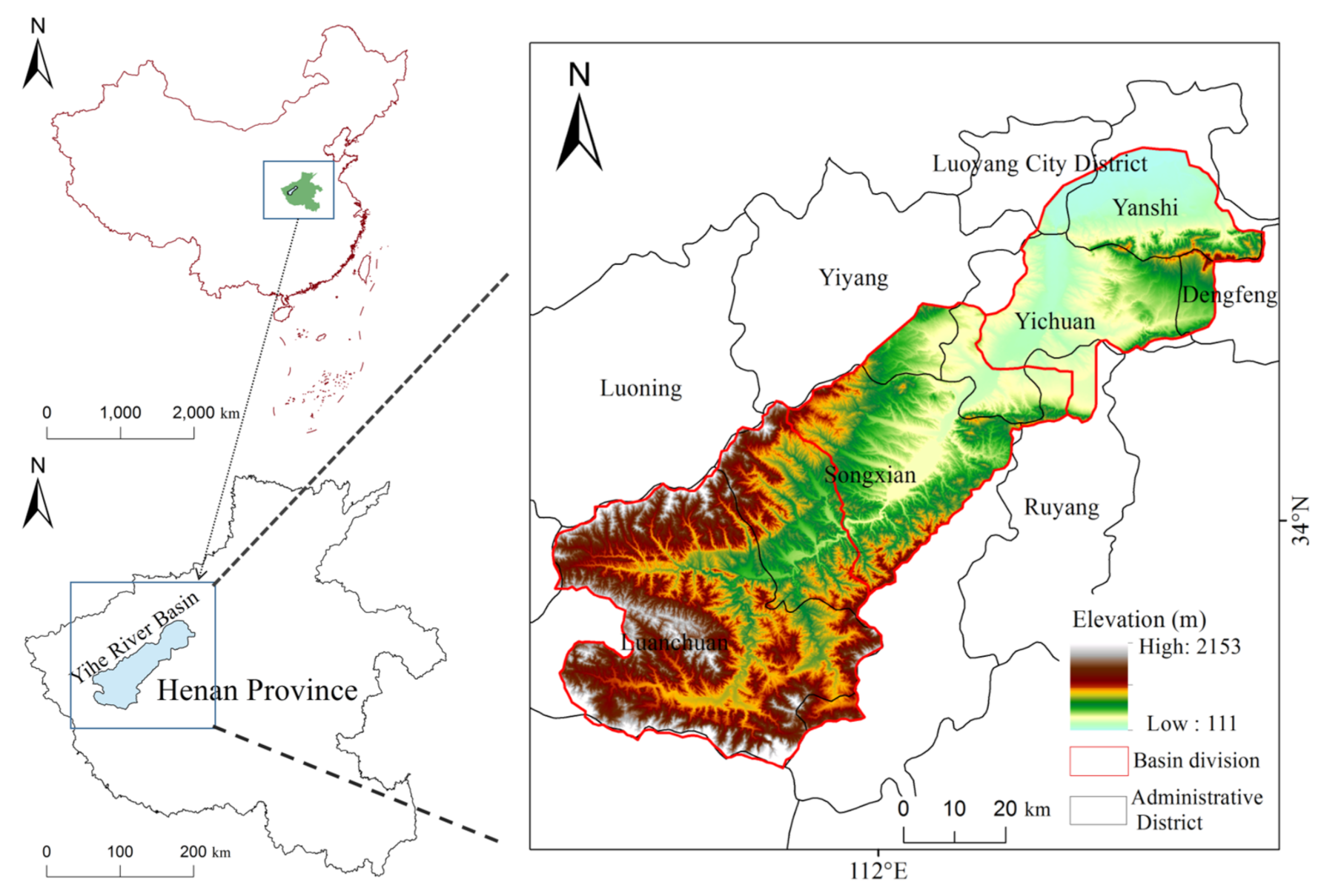
2.1. The Study Area

The Yihe River is one of the tributaries of the Luohe River, a tributary of the South Bank of the Yellow River in China. The geographical coordinates of this river are N 33°39′–34°41′ and E 111°19′–112°54′ (Figure 1), originating from the Taowan Town, Luanchuan at the southern foot of the Xiong’er Mountain, flowing through Songxian and Yichuan, and winding at the southern foot of the Xiong’er Mountain and the northern foot of the Funiu Mountain. The Yihe River has a total length of 264.88 km and a drainage area of more than 6100 km2. The runoff is particularly affected by precipitation (most of the precipitation is concentrated in June to August yearly), as well as topography, vegetation, and production activities. The Yihe River forms a unique landscape ecosystem of “mountain–hill–plain” from upstream to downstream. The ecological environment is also complex and fragile. From the administrative divisions, the Yihe River Basin mainly involves Luanchuan, Songxian, Yichuan, and Yanshi, as well as parts of Yiyang, Ruyang, Dengfeng, and Luolong. The total population of the Yihe River Basin in 2018 was 2.4221 million, with a gross national product of 133.637 billion yuan. For identifying spatial heterogeneity of ecosystem service supply, demand and risks, we divided the basin into upper, middle, and lower regions. First, based on the elevation data of Yihe River Basin, sub-basins were extracted and obtained. Then, taking sub-basins as units and combining the geomorphic type, we divided upper, middle, and lower regions. The upper reaches are mainly mountain valleys in Luanchuan. The middle reaches are mainly loess hilly area and stony hilly area. The lower reaches are mainly plain with fertile soil and is the main grain producing area of the river basin.

2.2. Data Collection and Collation

The data required for this study mainly include three land use/land cover remote sensing monitoring data in the Yihe River Basin, which are obtained from the Resource and Environment Science and Data Center of the Chinese Academy of Sciences (http://www.resdc.cn/, accessed on 10 October 2020), demonstrating a resolution of 30 m. The remote sensing image data were interpreted by using supervised classification and man–machine interactive methods and were verified via field selection, resident inter-views, and Google Earth high-resolution remote sensing images. The overall accuracy of these data was more than 85%. Digital elevation model (DEM) data originate from the geospatial data cloud (http://www.gscloud.cn/, accessed on 10 October 2020). Meteorological data mainly include those of precipitation and temperature, which respectively come from the China Meteorological Data Service Center (http://data.cma.cn/, accessed on 10 October 2020) and the National Earth System Science Data Center (http://www.geodata.cn/, accessed on 10 October 2020). The normalized difference vegetation index (NDVI) was calculated by reflectance in the near-infrared and red wavelengths, which was sensitive to green leaf area and surface vegetation coverage and could be used in ecological research. The NDVI data are obtained from the Earth Big Data Science Engineering Data Sharing Service System (http://databank.casearth.cn/, accessed on 10 October 2020), with a resolution of 30 m. The soil texture and other data come from the Chinese soil dataset based on the Harmonized World Soil Database. The population, food production, energy consumption, water resource consumption, and socio-economic data of each township in the study period were derived from the statistical yearbooks of counties (districts) included in the study, namely the statistical yearbooks of Henan Province and the Henan Provincial Water Resources Bulletin. The grid size of the different data sources is different and to stabilize the model outputs, the grid size we used in the spatial analysis is 1 km × 1 km. Moreover, after comparing the spatial and temporal patterns of ecosystem services under different grid size, we found that 1 km × 1 km grid scale can highlight the spatial differences of ecosystem services in our site (Table 1).

2.3. Research Framework

By integrating ecosystem service supply and demand evaluation, our study attempts to divide ecosystem service supply–demand risk management zones and offer policy decisions based on the proposed framework (Figure 2). We selected four ecosystem services—water yield, carbon sequestration, food production and soil conservation—following the criteria presented in Section 2.4.1. Based on the research framework, we first evaluated the supply and demand levels of the four ecosystem services by applying correlated models and then highlighted the spatial-temporal changes in each ecosystem service. Second, an ecosystem service supply–demand ratio was created to identify the situation of supply and demand matching. Third, we constructed and quantified ecosystem service supply–demand risk index and divide ecosystem service supply–demand risk management zones based on the risk levels to provide visual and effective information for ecosystem management and decision-making.

2.4. Evaluation and Mapping of Ecosystem Services Supply and Demand

2.4.1. Selection of Ecosystem Services

Based on the Millennium Ecosystem Assessment [54], more than twenty kinds of ecosystem services were listed and could be classified into provisioning services, regulating services, supporting services and cultural services. We only chose four typical and representative services, including water yield (provisioning service), carbon sequestration (regulating service), food production (provisioning service), and soil conservation (regulating service) according to the feasibility of their quantification, the availability of data and the importance of ecosystem services. The explanation was as follows. Because our research objective was identifying ecosystem service supply–demand risks, the selected ecosystem service needs to be quantified from both supply and demand sides and the four ecosystem services satisfied the condition. Moreover, water yield was a key service because Yihe River Basin was located in a semi-arid area and water yield can potentially mitigate the risks brought by drought. Carbon sequestration was conducive to mitigate the climate change, and ecosystems of our site were very sensitive to climate changes, so carbon sequestration also was an important service. Especially in recent years, carbon emissions caused by human activities continuously grew in this area, and the local government undertook the huge responsibility of carbon emission reduction and carbon neutral. Yihe River Basin was located in Henan Province, which was ‘food store’ of China, so our site had good agricultural foundation and sustaining food security belonged to the region responsibility. The proportion of cropland was about 40% and the amount of food supply was double of food demand in Yihe River Basin. Our site was a self-sustaining region in terms of food supply, so food production service was directly related to the local residents’ well-being, and also, key ecosystem services. Our site had a unique landscape ecosystem of “mountain–hill–plain” and soil conservation was selected given that the altitude difference between mountain and plain can lead to considerable soil erosion.

2.4.2. Water Yield

Water Yield Supply

InVEST (integrate valuation of ecosystem services and tradeoffs) is a suite of free, open-source software models used to map and value the goods and services from nature that sustain and fulfill human life [48]. Water yield module in the InVEST model has wide and matured application. This paper uses the water yield module in the InVEST model to evaluate the supply levels of water yield in the Yihe River Basin. The model is based on the water balance method to calculate the water yield of each grid by subtracting the actual evaporation from rainfall.
The water yield supply calculation model is presented as follows [48].
W Y ( x ) = ( 1 A E F ( x ) P ( x ) ) × P ( x )
A E F ( x ) P ( x ) = 1 + P E T ( x ) P ( x ) 1 + P E T ( x ) P ( x ) w 1 w
P E T ( x ) = K c ( x ) × E T O ( x )
W ( x ) = A W C ( x ) × Z P ( x ) + 1.25
where WY(x) is the water yield of grid x (mm); AEF(x) is the actual annual evapotranspiration of the grid unit x (mm); P(x) is the annual precipitation of the grid unit x (mm); PET(x) is the potential evapotranspiration of grid unit x; Kc(x) is the crop evapotranspiration coefficient; ETO(x) is the reference (crop) evapotranspiration; AWC(x) is the available water content of plants; W(x) is an empirical parameter that can be expressed as linear function of AWC∗N/P, where N is the number of rain events per year, and P is the annual precipitation; Z is an empirical constant, sometimes referred to as “seasonality factor”, which captures the local precipitation pattern and additional hydrogeological characteristics. It is positively correlated with N, the number of rain events per year [55]. The 1.25 term is the minimum value of W(x), which can be seen as a value for bare soil. In this model, land use/land cover, precipitation, soil texture and soil effective rooting depth raster data are needed.

Water Yield Demand

The demand for provisioning services can be captured by consumption [1]. The water yield demand of the Yihe River Basin is water consumption. According to the per capita comprehensive water consumption indexes in the “Henan Province Water Resources Bulletin,” the per capita comprehensive water consumption was calculated from the per capita water consumption of urban comprehensive living, the water consumption of rural residents, the average water consumption of farmland irrigation per hectare, and the industrial water consumption per 10,000 yuan of GDP. Combined with the grid data of population density, the quantitative map of water yield demand in corresponding years was obtained.
The water yield service demand model is calculated as follows [53]:
D W = D p w c × ρ p o p
where Dw is the water demand (m3), Dpwc is the annual per capita comprehensive water consumption in the study area (m3), and ρpop is the grid population density (person km−2).

2.4.3. Carbon Sequestration

Carbon Sequestration Supply

The carbon sequestration function of the ecosystem refers to the function of the natural ecosystem to absorb carbon dioxide in the atmosphere to synthesize organic matter and fix the carbon in plants or soil. This paper uses the net ecosystem productivity (NEP) method to calculate the carbon sequestration of terrestrial ecosystems. Net ecosystem productivity is an important scientific indicator for quantitative analysis of ecological carbon sinks. NEP is calculated in this paper by the conversion coefficient of net primary productivity (NPP) and NEP. NPP was estimated with the Carnegie Ames Stanford Approach (CASA). CASA is a typical model of light use efficiency, and it needs relatively few parameters. Moreover, some parameters do not require actual measurement and can be obtained from remote sensing data [56]. The supply of carbon sequestration consists of forests, grasslands, wetlands and soil carbon sequestration.
Carbon sequestration in forests, grasslands, and wetlands is calculated as follows [56]:
N E P = α × N P P
N P P ( x , t ) = A P R A ( x , T ) × ε ( x , t )
where NEP is the net ecosystem productivity (t·C/a), NPP is the net primary ecosystem productivity (t·C/a), α is the conversion coefficient of NPP and NEP, the value in Henan province can be capture in Ouyang et al. [6]. NPP(x,t) is the net primary productivity of pixel x in month t (g·C·m−2); APRA(x,t) is the photosynthetically active radiation of pixel x in t month (MJ·m−2), which can be calculated from NDVI;ε x , t is the actual light energy utilization rate of pixel x in t month (g·C·MJ−1), which is determined by land cover, temperature and precipitation. In this model, NDVI, land use/land cover, precipitation and temperature raster data are needed.
Soil carbon sequestration is calculated as follows [6]:
S i = C S C S + F C S + G S C S + W C S
C S C S = ( B B S + S C S R N + P R × S C S R S ) × S C
F C S = F C S R × S F
G S C S = G S R × S G
W C S = S C S R i × S W i
where Si is the amount of soil carbon sequestration (t·C/a); CSCS is the amount of carbon sequestration in farmland soil (t C/a); FCS is the amount of carbon sequestration in forests and shrubs (t·C/a); GSCS is the carbon sequestration of grassland (t·C/a); WCS is the carbon sequestration of wetland (t·C/a); BBS is the rate of carbon sequestration in farmland soil without carbon sequestration measures (t C·ha−1a−1), SCSRN is the soil carbon sequestration rate of farmland with chemical nitrogen fertilizer and compound fertilizer (t C·ha−1a−1); SCSRS is the rate of soil carbon sequestration in farmland with all straw returned to the field (t C·ha−1a−1 ); PR is the promotion rate of returning farmland straw to the field (%), which is valued as 62.63% based on the actual situation of our site in Henan province; SC is the area of farmland (ha); FCSR is the soil carbon sequestration rate of forests and shrubs (t C·ha−1a −1); SF is the area of forest and shrub (ha); GSR is the soil carbon sequestration rate of grassland (t C·ha−1a−1); SG is grassland area (ha); SCSRi is the carbon sequestration rate of the wetland in the i category (t C·ha−1a−1); SWi is the area (ha) of the wetland in the i category. The value of FCSR and GSR, and SCSRi result from the research results of Ouyang et al. [6] in Henan province or Eastern China. In the calculation process of soil carbon sequestration, land use/land cover, chemical nitrogen fertilizer and compound fertilizer data are needed.

Carbon Sequestration Demand

According to the energy consumption and residents’ eight major consumption data in “Henan Provincial Statistical Yearbook,” the comprehensive carbon emissions per capita in Henan Province were calculated following the approaches in Henan Province [57]. The carbon emissions per capita were combined with the raster data of population density to obtain a quantitative map of carbon sequestration demand for the corresponding year.
Carbon sequestration demand model [53]:
D C = D p c f × ρ p o p
where DC is the demand for carbon sequestration services (t), Dpcf is the per capita comprehensive carbon emissions quantity (t), and ρpop is the population density of the grid (person·km−2).

2.4.4. Food Production

Food Production Supply

Food production is an important provision in ecosystem services and has a substantial impact on human well-being. Existing studies [52,53] have shown a significant linear correlation between the yield of crops and livestock products and the NDVI. The total output of crops, such as grain, oilseeds, and vegetables, were distributed in accordance with the ratio of the grid NDVI value to the total arable land NDVI value. Meanwhile, the output of livestock products, such as meat and milk, were distributed on the basis of the ratio of the grid NDVI value to the total grassland NDVI value. The aquatic product output was allocated on the basis of the ratio of grid NDVI value to the water area total NDVI value ratio. Such allocations were provided to characterize the food supply capacity of each grid and obtain the source of food supply services in different years.
Food production supply model [52]:
G i = G s u m × N D V I i N D V I s u m
where Gi is the food supply of grid i, Gsum is the total output of grain, meat, milk and water products, NDVIi is the normalized vegetation index of the grid i, and NDVIsum is the sum of NDVI values of cultivated land, grassland or waters.

Food Production Demand

The food production demand was estimated by multiplying the per capita food demand by the population density. Meanwhile, the per capita food demand was estimated by using the lowest value of the ideal range of per capita daily food consumption under a reasonable dietary structure in the “Chinese Resident Dietary Guidelines 2016.” In the guidelines, daily meals should include 250~400 g of cereals and potatoes, 300~500 g of vegetables, 200~350 g of fruits, 300g of milk, and 120~200 g of meat and eggs. The lowest value of the ideal range of per capita daily food consumption was selected because the per capita income in our site was below the average level of China.
Food production demand model [53]:
D F = D p f c × ρ p o p
where DF is the food demand (t), Dpfc is the per capita food demand (t), and ρpop is the population density of the grid (person·km–2).

2.4.5. Soil Conservation

Soil conservation service was defined as ecosystems that protect soil, reduce rainwater erosion and reduce soil loss through their structures and processes. The revised universal soil loss equation (RUSLE) took almost all factors of soil erosion [58,59]. The parameters in the equation were easy to access. The estimated results of the equation had high precision. RUSLE has been widely used in the basin scale and was used in the current study to estimate the amount of regional soil conservation and erosion. The difference between the potential and the actual erosion amounts was used to represent the supply of soil conservation, and the actual soil erosion was taken as the demand of soil conservation [60,61].
Soil conservation supply model [58,60]:
S C = R K L S U S L E = R × K × L S R × K × L S × C × P
Soil conservation demand model [58,60]:
U S L E = R × K × L S × C × P
where SC is the amount of soil conservation; RKLS and USLE are the potential and actual erosion amounts (t·hm−2·a−1), respectively; R is the rainfall erosion factor (MJ·mm·hm−2·h−1·a−1); K is the soil erodibility factor (t·hm2·h·MJ−1·mm−1·hm−2); LS is the terrain factor; C is the surface vegetation coverage factor; and P is the water and soil conservation management factor. In this model, land use/land cover, DEM, NDVI, precipitation soil texture, soil organic matter content and soil types of raster data are needed.

2.5. Ecosystem Service Supply–Demand Ratio

This paper adopts the ecosystem service supply–demand ratio (ESDR) [62,63,64,65] to measure the relationship between the supply and demand of ecosystem services. Such measurement aims to establish the supply–demand ratio formula of ecosystem services to compute for the surplus and deficit changes in the supply and demand of ecosystem services in the Yihe River Basin. A positive value of ESDR indicates an oversupply of a certain ecosystem service, that is, a surplus; a negative value indicates that supply exceeds demand, that is, a deficit. A value of zero indicates a balanced state of supply and demand.
E S D R = S D ( S max + D max ) / 2
where S is the supply of a certain ecosystem service, D represents the demand for a certain ecosystem services, Smax refers to the maximum grid value of the assessed a certain ecosystem service supply in our site, and Dmax is the maximum grid value of the assessed demand for a certain ecosystem service in our site.
The comprehensive ESDR (CESDR) integrated the supply and demand of several different ecosystem services to determine the supply–demand matching status of the overall ecosystem services and was calculated as the arithmetic average of ESDR [63].
C E S D R = 1 n i = 1 n E S D R i
where n represents the number of ecosystem services (in this study, n = 4), and ESDRi is the supply–demand ratio of various types of ecosystem services.

2.6. Risk Levels of Ecosystem Service Supply and Demand

This paper constructs an ecosystem service supply–demand risk index system based on Maron et al. [49] and other classification standards and classifies ecosystem service supply–demand risk levels according to three indicators of ecosystem service supply trends, supply–demand ratios, and supply–demand ratio trends. The ecosystem service supply trend can express the absolute change in regional ecosystem service supply. If the trend is larger than zero, then the ecosystem service supply increases during this period; if the difference is zero, then the supply of ecosystem services remains unchanged during this period; if the trend is less than zero, then the ecosystem service supply decreases during the period. The supply–demand risks of ecosystem services were divided into I–V levels for spatial mapping (Table 2).
The ecosystem service supply–demand ratio can express the regional ecosystem service supply deficit or surplus. Critically endangered level, endangered level and stable but undersupplied level belongs to the supply deficit, while vulnerable level and secure level belong to supply surplus. The detailed explanations are as follows.
If the supply–demand ratio of ecosystem services is less than zero, then the demand for ecosystem services is larger than the supply; thus, the regional ecosystem services supply cannot meet the demand. Under these conditions, if the supply–demand ratio declines, then the supply–demand risk level of ecosystem services in the region is critically endangered; if the supply–demand ratio trend increases while the supply trend decreases, then the supply and demand risk level of ecosystem services in the region is endangered; if the supply–demand ratio declines while the supply trend rises, then the region is in a state of insufficient supply. A supply–demand ratio larger than or equal to zero indicates that the supply capacity of ecosystem services is larger than or equal to the demand capacity to meet social needs. In this case, if the supply–demand ratio shows a downward trend, then the supply and demand risk level of ecosystem services in the region is vulnerable; if the supply–demand ratio shows an upward trend, then the supply and demand risk level of ecosystem services in the region is secure.
Considering the flow of ecosystem services between upper and downstream areas in the River Basin, multiple spatial-scale approach is applied to analyze the ecosystem service supply–demand risk levels, including grid scale, sub-basin scale and entire-basin scale. Watershed is an integrated system thus ecosystem services in one area might be consumed by other areas. In order to more completely express the ecosystem service supply–demand risk status in our site, our study takes grid, sub-basins and entire basin as the unit, analyzes the proportion of high-risk level area and supply–demand risk status in each scale.

3. Results

3.1. Spatial-Temporal Changes in the Ecosystem Service Supply and Demand

3.1.1. Water Yield Supply and Demand

The spatial pattern of water yield supply capacity is high in the southwest and low in the northeast, and the upstream water production supply capacity is strong in our site (Figure 3). The water yield supply is consistent with the distribution of lakes and other water bodies. The total water yield of our site from 2000 to 2018 decreased from 1071 hm3/a in 2000 to 902 hm3/a in 2018, demonstrating a reduction of 15.78%. However, the annual water output in 2018 increased by only 2.85% compared with that in 2008, first decreasing and then increasing in the segment. Meanwhile, the total annual water output in our site from 2000 to 2018 decreased overall (Table 3). In the same year, the water yield of the Yihe River Basin showed a large difference in space, with the unit water yield of upstream > middle stream > downstream in the basin. From 2000 to 2008, the water yield in the upper, middle, and downstream reaches respectively decreased by 17.76%, 20.61%, and 20.61%. The water yield in the upper, middle, and lower reaches decreased from 2000 to 2008, and the reduction in the upper reaches was small. From 2008 to 2018, the upper, middle, and lower reaches showed a slow upward trend, of which the downstream water yield had a large increase of 6.31%, and the upper and middle reaches of the increase were 2.33% and 5.92%, respectively.
The distribution of water yield demand (Figure 3) reveals the spatial pattern of water yield demand in the Yihe River Basin from 2000 to 2018. Overall, the demand for water yield in the northeast and southwest was respectively high and low, and the downstream area had a large demand for water yield. Water demand dropped slowly from 432 hm3/a in 2000 to 431 hm3/a in 2008, but that in 2018 increased by 33.56% compared with 2000, showing a trend of first decreasing and then increasing in the section. The total water demand of our site increased from 2000 to 2018 overall (Table 3). In the same year, the water demand of our site showed a large difference in space, the unit water demand of the basin was opposite to the water yield, and the downstream water demand was the largest. Except for a slight decrease in the downstream, water demand in other regions slightly increased during 2000–2008. The water demand from 2000 to 2018 in the upper, middle, and lower reaches increased to varying degrees, and the midstream demand increased by a maximum of 38.56%. The upstream and downstream water demands increased by 31.61% and 31.77%, respectively.

3.1.2. Carbon Sequestration Supply and Demand

The supply of carbon sequestration in our site showed a spatially decreasing trend from southwest to northeast from 2000 to 2018, and high-value areas were found in the northeast of the river basin (Figure 4). The supply of carbon sequestration mainly comes from vegetation and soil [66,67]. The high values of carbon sequestration were mostly concentrated in Luanchuan. The vegetation coverage in these areas was high, and the area of forest land is large. The vegetation types were mainly cork oak, broad miscellaneous and Chinese pine [68]. The watershed carbon sequestration supply was consistent with the vegetation distribution. The total amount of carbon sequestration supply decreased from 4.10 × 10⁸ t·C/a in 2000 to 4.08 × 10⁸ t·C/a in 2018. The total supply in 2008 was 3.97 × 10⁸ t·C/a; therefore, the change in supply from 2000 to 2018 first decreased and then increased (Table 4). The total supply of carbon sequestration in the study area decreased by 0.49% from 2000 to 2018.
The total demand for carbon sequestration increased from 7.12 × 10⁵ t·C/a in 2000 to 1.63 × 10⁶ t·C/a in 2008 and then increased to 2.42 × 10⁶ t·C/a in 2018 (Table 4). The demand for carbon sequestration showed an overall upward trend, and the downstream areas were substantially higher than those in the upper and middle reaches (Figure 4). High values were mainly concentrated in the middle and lower reaches of the basin. The middle and lower reaches were densely populated and highly urbanized, which consumed additional energy, leading to substantial pressure on carbon emission reduction. In addition, the demand for carbon sequestration increased with the development of the middle and lower reaches of the population economy.

3.1.3. Food Production Supply and Demand

Figure 5 shows that the spatial pattern of food production in our site from 2000 to 2018 was stable, spatially high in the northeast and low in the southwest, and the supply capacity of downstream food production was higher than that in the upper and middle reaches. The supply of food production in our site in 2000 was 15.50 × 10⁸ kg/a, which increased to 21.90 × 10⁸ kg/a in 2018. The value in 2018 decreased by 0.06% compared with that in 2008 (Table 5). The decline in the supply of food production from 2008 to 2018 was mainly caused by the decrease in the cultivated area. In the same year, the supply of food production in the study area were quite different in space. The areas with strong supply capacity were concentrated in the downstream areas, and the supply capacity in the upstream was small. The downstream supply in 2000 and 2018 respectively accounted for 44.29% and 44.30% of the entire study area. The food production and supply level in the watershed were stable in time and space.
The spatial distribution of demand for food production in the Yihe River Basin was stable from 2000 to 2018, showing an increasing trend from southwest to northeast. The high values were mainly concentrated in Yanshi and Yichuan (Figure 5). The demand for food production in the Yihe River Basin gradually increased from 9.32 × 10⁸ kg/a in 2000 to 11.60 × 10⁸ kg/a in 2018, and the demand increased by 24.46% (Table 5). In the same year, high-demand areas were concentrated in the middle and lower reaches of the basin, and the upstream demand was small. The demand for food production per unit area of the basin was uneven, but the law was consistent.

3.1.4. Soil Conservation Supply and Demand

The distribution of soil conservation in our site was stable from 2000 to 2018 and only demonstrated minimal changes (Figure 6). The results of soil conservation supply showed that forest land was the highest, followed by grassland, and water and construction land were low. The supply of soil conservation services changed from 9.47 × 10¹¹ t/a in 2000 to 9.48 × 10¹¹ t/a in 2018, and the amount of soil conservation first decreased and then increased (Table 6). From 2000 to 2008, the areas with a reduced supply of soil conservation were concentrated in the areas with large topographic undulations in the upper reaches of Luanchuan. The areas with an increased supply of soil conservation were mainly the downstream flat areas. The supply of soil conservation in the middle and lower reaches gradually increased from 2008 to 2018, and the supply of Miaozi, Tantou, Taowan, and Shimiao Towns in the upper reaches considerably decreased. Most of the high values of soil conservation supply in the Yihe River Basin were concentrated in the upper reaches. The upstream forest land resources were rich, the soil structure was good, and the disturbance of upstream human activities was small, which can account for the high amount of soil conservation in the upper reaches. However, the amount of soil conservation in cultivated land, construction land, and water areas, which were located in the middle and lower reaches of the region, was low. The terrain was flat; therefore, the amount of soil conservation was small.
The total demand for soil conservation in 2000 was 5.33 × 10⁹ t/a, which changed to 5.37 × 10⁹ t/a in 2018. The demand increased first and then decreased (Table 6). The area where demand for soil conservation increased accounted for 30.65%, and the decreased area was 34.67% from 2000 to 2008. From 2008 to 2018, the area with increased demand for soil conservation was 19.93%, and the decreased area was 34.77%. This finding indicates a slight decrease in the soil conservation demand of the watershed in recent years. The demand for soil conservation in our site showed spatial differences from 2000 to 2018. The areas with high demand for soil conservation were mainly on both sides of the river in the upper and middle reaches and parts of the northeast of the lower reaches (Figure 6). The large difference in the spatial distribution of the demand for soil conservation is mainly due to the slope of the terrain. Areas with large terrain undulations had substantial soil erosion, and high demand for soil conservation. In addition, the areas with high demand were mostly at the junction of different land types. Meanwhile, the areas with poor vegetation coverage, broken terrain, and low demand for soil conservation were mainly concentrated in the lower reaches primarily due to the flat terrain in the lower reaches and the existence of several construction land.

3.2. Supply and Demand Matching of Ecosystem Services

3.2.1. Supply and Demand Matching of Individual Ecosystem Services

The water yield supply–demand ratio of the Yihe River Basin from 2000 to 2018 maintained high and low spatial patterns in the southwest and northeast, respectively (Figure 7). The upstream maintained a high level of supply–demand ratio. Affected by nature and society, the demand for water in the middle and lower reaches was larger than the supply of water yield, which is in a state of water shortage, and the scope of the deficit increased. The middle and lower reaches of the water demand cannot be met. The regional differentiation was serious, and the supply distribution was uncoordinated, causing the gradual increase in deficits in the downstream.
The supply of carbon sequestration in our site was far larger than the demand (Table 4). The matching status of supply and demand in 2000, 2008, and 2018 is shown in Figure 6. From the spatial distribution viewpoint, the upstream supply and demand matched well in each year. The area of mismatch between supply and demand in 2000 and 2018 was larger than that in 2008. The area where supply exceeded demand was 94.97% in 2008. The supply–demand matching of carbon sequestration markedly improved in 2018 compared with that in 2000. Overall, the supply of carbon sequestration was high in the areas with dense vegetation, and the mismatch areas were mostly in the areas with rapid urbanization process and the two sides of the Yihe River Basin.
The spatial pattern of the supply–demand ratio of food production from 2000 to 2018 was lower in the southwest region than in the northeast during the study period, the supply in the middle and lower reaches was larger than the demand, and the supply in the upper reaches was insufficient (Figure 7). The supply in the study area met the demand during the study period, and the supply level was the highest in 2008. The supply–demand ratio of food production in our site fluctuated around a value of zero, and the degree of matching between supply and demand was good, which is close to a balanced state.
The supply–demand ratio of soil conservation was generally at a high level from 2000 to 2018, with the highest in the southwest of the river basin (Figure 7). The area with a deficit in soil conservation accounted for a small proportion of the total area, and the supply and demand of soil conservation in our site maintained a high matching level.

3.2.2. Supply and Demand Matching of Comprehensive Ecosystem Services

Figure 8 and Table 7 show the comprehensive supply–demand ratio of the four ecosystem services in our site from 2000 to 2018. The comprehensive supply–demand situation of ecosystem services in the entire river basin shows that supply exceeded demand, and the comprehensive supply–demand ratio gradually decreased from 2000 to 2018. The difference between supply and demand matching was observed in the same year, the upstream comprehensive net supply value was the highest, and the middle and downstream comprehensive net supply values were low. The comprehensive supply–demand ratio of upstream ecosystem services increased during the study period, but the comprehensive supply–demand ratio of mid and downstream ecosystem services decreased. The increase in demand in the middle and lower reaches led to a worsening of their deficits, reflecting the gap in social and economic development in different regions of the river basin.

3.3. Supply–Demand Risks of Four Ecosystem Services

3.3.1. Supply–Demand Risks at the Grid-Scale

The supply–demand risk levels of various ecosystem services in the three periods of 2000–2008, 2008–2018, and 2000–2018 in the Yihe River Basin are obtained by combining the three indicators of supply–demand ratio, supply–demand ratio trend, and supply trend (Figure 9). Water yield was mainly vulnerable and critically endangered from 2000 to 2018, with high-risk and low-risk grades accounting for 50.02% and 49.98%, respectively. Low-risk grades were concentrated upstream, while high-risk areas were concentrated in the middle and lower reaches. The proportions of high-risk and low-risk grades of water yield in 2000–2008 and 2008–2018 were 49.64%, 50.36%, 50.02%, and 49.98%, indicating the slight increase in the supply–demand risks of water yield.
The carbon sequestration was mainly at a secure level from 2000 to 2018, and the proportions of high-risk and low-risk levels were 6.39% and 93.61%, respectively. The proportion of high-risk and low-risk grades in 2008–2018 is the same as that in 2000–2018. However, the proportion of undersupplied grades in high-risk areas is higher than that in 2000–2018, while that of endangered grades in 2000–2018 is higher than that in 2008–2018. The carbon sequestration was mainly based on vulnerable and secure levels from 2000 to 2008, with high-risk and low-risk levels accounting for 5.03% and 94.97%, respectively. The overall supply–demand risk of carbon sequestration in the basin was low, but the high-risk area of carbon sequestration slightly increased in recent years.
The food production from 2000 to 2018 was mainly secure but insufficiently supplied, with high-risk and low-risk grades accounting for 52.68% and 47.32%, respectively. Low-risk grades were concentrated in the midstream and downstream, and high-risk areas were concentrated upstream. The proportions of high-risk and low-risk levels in 2000–2008 and 2008–2018 were 50.15%, 49.85%, 52.61%, and 47.39%. The supply–demand risk of food production increased from 2008 to 2018, and the secure level was transformed into a vulnerable level.
The supply–demand risks of soil conservation mainly demonstrated secure levels from 2000 to 2018. The proportions of high-risk and low-risk levels were 0.44% and 99.56%, respectively. Meanwhile, the proportions of high-risk and low-risk levels in 2000–2008 and 2008–2018 were 0.54%, 99.46%, 0.44%, and 99.56%, indicating that the soil conservation risk level was stable and improved in 2008–2018.

3.3.2. Supply–Demand Risks at the Sub-Basin Scale

Considering the fluidity of ecosystem services, this study used sub-basin as a unit to express the supply–demand risk status of ecosystem services in our site (Figure 10). The supply–demand risks of water yield in the sub-basin from 2000 to 2018 were mainly critically endangered and vulnerable, and the number of high-risk and low-risk sub-basins each accounted for 50%. Considering periods, the water yield supply–demand risk of the Sub-Basin 3 changed from an endangered to a critically endangered level, and the sub-basin 18 changed from vulnerable to secure level. The supply–demand risks of carbon sequestration in the sub-watershed from 2000 to 2018 were mainly safe and vulnerable levels. The supply–demand risks of carbon sequestration in different periods were in a low-risk state and the supply could meet the needs of human carbon emissions. The food production supply–demand risk levels from 2000 to 2018, except for the Sub-Basin 24, were all low-risk levels, of which Sub-Basins 3, 8, and 23 were vulnerable, and the rest were secure levels. The supply–demand risk level of food production in 2008–2018 worsened compared with that in 2000–2008, and the secure level transformed to a vulnerable level. The supply–demand risks of soil conservation in the sub-basins were low risk at different times from 2000 to 2018, and the safety level demonstrated the most risk grade. Overall, the supply–demand risks of the Sub-Basins 3 and 10 gradually improved.

3.3.3. Supply–Demand Risks in the Entire Basin

The supply–demand risks of ecosystem services can be determined in accordance with the supply trend, supply–demand ratio, and supply–demand ratio trend of ecosystem services in the entire river basin from 2000 to 2018 (Table 8). On the scale of the entire river basin, the supply–demand risk levels of the four ecosystem services were slightly consistent. The supply–demand risk levels of water yield, carbon sequestration, and soil conservation were vulnerable, but the food production supply–demand risk level was secure.

3.4. Spatial Management Zoning Based on Ecosystem Service Supply–Demand Risks

By using spatial overlay analysis on four ecosystem services supply–demand risk levels in sub-basin scale from 2000 to 2018, the eight supply–demand risk management zones of the Yihe River Basin were obtained (Figure 11). The first category is Sub-Basin 8, where the water yield was critically endangered, and the three other services were at the vulnerable level. The second category includes Sub-Basins 4, 5, 6, 7, 9, 13, and 26, where water yield was critically endangered, and the three other services were at the vulnerable level. The third category is the Sub-Basin 3, wherein the water yield was critically endangered, the food production was vulnerable, and the two other services were at a secure level. The fourth category includes Sub-Basins 1, 2, 10, and 14, where water yield was critically endangered, and the three other services were at the secure level. The fifth category is Sub-Basin 24, wherein the food production was critically endangered, the water yield and carbon sequestration were vulnerable, and the soil conservation was at a secure level. The sixth category is Sub-Basin 23, wherein the four services were at the vulnerable level. The seventh category is Sub-Basin 25, which refers to water yield and food production as the vulnerable levels, and the rest were secure levels. The eighth category includes Sub-Basins 11, 12, 15, 16, 17, 18, 19, 20, 21, and 22, wherein water yield was vulnerable, and the three other services were at the secure level.

4. Discussion

4.1. Framework of Supply–Demand Risks Evaluation System of Ecosystem Services

The risks of ecosystem services to human beings, the degree of risks, and the available trends need to be determined to provide a strong basis for ecosystem service risk management and related policy formulation. Some conceptual models, such as the EPPS (ecosystem properties, potentials, services, and benefits) framework [69], the delivery chain of ecosystem services [17], and the comprehensive assessment framework for the ecosystem service supply and demand [20,70,71], are created to view the supplier and demand sides of integrated ecosystem services. These conceptual models provide a theoretical and practical basis for the research on the supply–demand risks of ecosystem services. The assessment of the supply–demand risks aim to link the supply–demand relationships and the risks of ecosystem services. Following this, we can divide the degree of risk faced by ecosystem services from the risk perspective and this provides a new viewpoint for the management of ecosystem services. Research on ecosystem service risks has received widespread attention in recent years. One focused on risk assessment based on the supply of ecosystem services, and the degree of reduction in supply is used as the basis for risk division. The other is based on the evaluation of the supply–demand relationship of ecosystem services, emphasizing the matching degree between supply and demand. The former is too simplistic and lacks consideration of human needs, complicating the use of research results in actual management. By contrast, the latter lacks practical case studies due to the difficulty in identifying the demand for ecosystem service. Our research constructed a framework to identify the supply–demand risk levels by analyzing the three indicators of supply–demand ratio, supply–demand ratio trend, and supply trend based on the quantification of the supply and demand of ecosystem services. The framework of ecosystem service supply–demand risks evaluation system is conducive to examining the change in time series and regional consumption of natural resources and the spatiotemporal evolution characteristics of ecosystem service supply–demand risks. The identification of the supply–demand risks of ecosystem services is also conducive to an overall grasp of the supply and demand status of regional ecosystem services and rational investment of limited resources into different risk zones to promote the sustainable development of regional ecosystems.
Based on the framework of supply–demand risks evaluation system, the ecosystem service supply–demand risk models were employed to assess the supply–demand risk levels of four services in the Yihe River Basin, including water yield, carbon sequestration, food production, and soil conservation. The spatial heterogeneity of the study area is strong. The upper reaches are mountainous areas with abundant forest resources, the middle reaches are loess hilly areas with abundant resources, and the lower reaches are plain areas, which are the main grain-producing areas. Dividing the supply–demand risk levels of ecosystem services in the river basin is conducive to the management of ecosystem services and the targeted implementation of policies. Moreover, the study integrated the supply–demand risk levels of four services on the scale of sub-basin for spatial management zoning of risks. The risk management zoning of the Yihe River Basin can identify the ecological and economic development problems faced by different river basins. Some Sub-Basins, such as the Sub-Basins 1, 2, 10, and 14, only face water shortages. However, some sub-basins encountered many ecological and environmental problems. For example, Sub-Basin 24 is facing the risk of food shortages and insufficient water resources. Therefore, the risk management division of the supply and demand of ecosystem services is helpful to the effective management of ecosystem services in a river basin.

4.2. Factors Affecting Supply–Demand Risks of Ecosystem Services

The factors affecting the supply–demand risks of ecosystem services in the Yihe River Basin involve natural ecosystems and socio-economic systems, including natural and socio-economic factors [20]. The supply and demand of the river basin show temporal and spatial heterogeneity due to natural and socio-economic factors. The difference of service types and the total amount in different times and geographical locations leads to considerable temporal and spatial effects of supply–demand risks. The upstream ecological background resources were satisfactory, and the water yield, carbon sequestration, and soil conservation supply levels were high because of the influence of the differences in the natural ecological characteristics of the basin. The downstream terrain was flat, and only the food production supply level was high. However, the demand for most ecosystem services in the downstream were high because of the high population density. For example, the supply–demand risk factors of water yield and carbon sequestration were mainly the natural ecological environment and population. The upstream mountainous areas were rich in water and forest resources, while the downstream plains were densely populated with large amounts of water consumptions and carbon emissions, resulting in uneven distribution of water yield and carbon sequestration supply and demand. Under the combined influence of the two factors, the supply–demand risk of water yield in almost all downstream sub-basins was critically endangered, and the supply–demand risk of carbon sequestration in most downstream sub-basins was vulnerable.
Changes in the supply–demand risks of ecosystem services at different time nodes are mainly affected by the human socio-economic system. The socio-economic system changes more drastically than the natural ecosystem on a short time scale [70]. Therefore, the demand-side drivers of ecosystem services (such as population growth and economic development) may have a larger impact on service supply–demand risks than supply-side drivers. For example, the increase in food production supply will be affected by social and economic factors, such as agricultural chemical inputs, a series of policies to benefit agriculture and agricultural science and technology innovation. Moreover, the demand for food production will be affected by the increase in population. Food production is strongly affected by the former; therefore, the supply–demand risks faced by food production have slightly improved in recent years. In addition, the supply level of soil conservation will also increase with the strengthening of ecological protection awareness and the impact of human ecological protection projects and policy implementation. Therefore, the supply–demand risks faced by soil conservation were also improved in some sub-basins in recent years.

4.3. Policy Enlightenment

Management divisions based on the supply–demand risks of multiple ecosystem services can reflect the risk levels of supply and demand of multiple ecosystem services. The risk level of supply and demand of ecosystem services in each sub-basin can be identified on the basis of the risk management zone, and the region can be guided to realize the rational allocation of resources. Based on eight risk management zones and characteristics of four ecosystem services supply–demand risk, we propose three guidelines of ecosystem services optimization in our site. The optimization suggestions help to realize the reasonable spatial allocation of resources between supply–demand risk zones through ecosystem service flow.
The sixth, seventh, and eight types of risk zones are core protected areas and the key to this is ecosystem conservation. Considering the Yihe River Basin, the supply and demand risks of the four ecosystem services in the three types of regions are all at a low-risk level and do not require many control measures. However, most of these areas are concentrated in upstream, which is an important ecological function area in the watershed. Therefore, monitoring water yield, carbon sequestration, and soil conservation, grasping the dynamic trend of the supply of different services, and strictly preventing their degradation are necessary. In addition, the conservation of water and forest resources should be emphasized. The habitat conditions in the upper reaches have a direct impact on the ecosystem services in the middle and lower reaches.
The fifth category of risk zone is the food production promotion area, and the key is development agriculture. Except for food production, ecosystem services in the fifth category of areas are at a low-risk level. In this category, focusing on changes in the supply level of food production, strengthening the integrated innovation of agricultural science and technology and the development of benefit farming policy, promoting the growth of food production in the region are necessary to reduce the supply–demand risk level of food production.
The first to fourth types of risk zones are water recharge promotion area and face the high risk of water shortages. The water resources are in short supply, and the supply–demand risk of water yield is high. From a spatial viewpoint, these areas mainly located in the middle and lower reaches, with convenient transportation and high population density. The intensity of urban development in each sub-basin is higher than that in the upstream sub-basin. Preventing excessive waste of water resources is necessary for the urbanization process. Areas with a high-risk level of water yield must form a sound water-saving policy, regulation, and standard system, raise people’s awareness of water-saving, adjust water prices in a timely and appropriate manner, and increase the repetition rate of water resources and the rate of ecological benefits. Moreover, water yield service supply–demand risk can be spatially regulated in the form of ecosystem service flow.

4.4. Limitations of the Research

The Millennium Ecosystem Assessment [54] has identified more than 20 types of ecosystem services, however, we only chose four key ecosystem services as representatives. If all ES are evaluated, it will take much time and manpower. Moreover, the supply–demand ratio of some ecosystem services cannot be calculated because of the different measurement units of supply and demand assessment results, making it difficult to assess ecosystem service supply–demand risks [51]. The appropriate methods quantifying ecosystem service supply and demand still need to further explore. The time series of ecosystem services supply levels basically consists of three data points because of discontinuity of remote sensing data. If the continuous data availability can be guaranteed, ecosystem service supply–demand risks of our site can be more fully and convincingly assessed. In the following research, we will conduct research on some other availability data. Moreover, due to the limitations of assessment methods, this study does not consider the questions of circular economy and exports of ecosystem services to the region. Although our site is a self-sustaining region and we have tried to analyze the ecosystem service supply–demand risks at different spatial levels (i.e., grid scale, sub-basin scale and entire basin), the impact of those questions on risk levels still need attention. In the following research, we will strive to optimize the supply and demand evaluation methods of ecosystem services.

5. Conclusions

This paper proposed a framework of supply–demand risks evaluation system of ecosystem services by integrating ecosystem service supply and demand evaluation. Our study attempts to evaluate ecosystem service supply and demand, divide ecosystem service supply–demand risk management zones and offer policy decisions by using the proposed framework.
(1) The spatial distributions of the supply and demand of four ecosystem services in the Yihe River Basin was stable but unmatched from 2000 to 2018. The food production supply levels in the middle and lower reaches and the upstream water yield, carbon sequestration, and soil conservation supply levels were high. However, most of the areas with high demand for ecosystem services were concentrated in downstream.
(2) The temporal changes of four ecosystem services in the Yihe River Basin from 2000 to 2018 are presented as follows. The supply of water yield and carbon sequestration in the Yihe River Basin decreased, while that of food production and soil conservation increased. The demand for the four ecosystem services also increased.
(3) The supply–demand risk levels of the four ecosystem services were secure or vulnerable on the entire watershed scale. However, spatial differences were found in the supply–demand risk levels on the sub-basin scale. A total of 50% of the sub-basin water yield supply–demand risks were at a high-risk level, and the risk areas were concentrated in the middle and lower reaches. The supply–demand risks faced by water yield slightly increased in recent years. The three remaining services were mainly at low-risk levels. However, the supply–demand risk level of food production remarkably changed from secure to vulnerable level in recent years, thus requiring attention.
(4) The Yihe River Basin was divided into eight types of supply–demand risk management zones based on the evaluation results of the supply–demand risks of ecosystem services, and each type of area has targeted land or environmental policies to the corresponding risks. The assessment of the supply and demand of ecosystem services from a risk perspective can integrate the information of natural ecosystems and socio-economic systems and provide scientific support for watershed spatial management.

Author Contributions

Conceptualization, Q.M. and H.W.; data curation, L.Z., E.C. and M.L.; Formal analysis, Q.M. and D.X.; funding acquisition, Q.M. and H.W.; methodology, H.W.; Visualization, L.Z.; writing—original draft, L.Z.; writing—review and editing, Q.M. and H.W. Q.M. and L.Z. contributed equally to this work. All authors have read and agreed to the published version of the manuscript.

Funding

This research was funded by the National Natural Science Foundation of China (41901259), Henan Science and Technology Think Tank Program (HNKJZK-2021-06B), and the special fund for top talents in Henan Agricultural University (30500425).

Institutional Review Board Statement

Not applicable.

Informed Consent Statement

Not applicable.

Data Availability Statement

The data presented in this study are available on request from the corresponding author.

Conflicts of Interest

The authors declare no conflict of interest.

References

  1. Bukhard, B.; Kroll, F.; Nedkov, S.; Müller, F. Mapping ecosystem services supply, demand and budgets. Ecol. Indic. 2012, 21, 17–29. [Google Scholar] [CrossRef]
  2. Redhead, J.W.; May, L.; Oliver, T.H.; Hamel, P.; Sharp, R.; Bullock, J.M. National scale evaluation of the invest nutrient retention model in the United Kingdom. Sci. Total Environ. 2018, 610–611, 666–677. [Google Scholar] [CrossRef]
  3. Wu, X.; Liu, S.; Zhao, S.; Hou, X.; Xu, J.; Dong, S.; Liu, G. Quantification and driving force analysis of ecosystem services supply, demand and balance in China. Sci. Total Environ. 2019, 652, 1375–1386. [Google Scholar] [CrossRef] [PubMed]
  4. Daily, G. Nature’s Services: Societal Dependence on Natural Ecosystems; Island Press: Washington, DC, USA, 1997. [Google Scholar]
  5. Wang, R.; Ouyang, Z. Social-Economic-Natural Complex Ecosystem and Sustainability. Bull. Chin. Acad. Sci. 2012, 27, 254, 337–345, 403, 404. (In Chinese) [Google Scholar]
  6. Ouyang, Z.; Song, C.; Zheng, H.; Polasky, S.; Xiao, Y.; Bateman, I.J.; Liu, J.; Ruckelshaus, M.; Shi, F.; Xiao, Y.; et al. Using gross ecosystem product (GEP) to value nature in decision making. Proc. Natl. Acad. Sci. USA 2020, 117, 14593–14601. [Google Scholar] [CrossRef] [PubMed]
  7. Su, C.; Wang, Y. Evolution of ecosystem services and its driving factors in the upper reaches of the Fenhe River watershed, China. Acta Ecol. Sin. 2018, 38, 7886–7898. (In Chinese) [Google Scholar]
  8. Wang, Z. Evolving landscape-urbanization relationships in contemporary China. Landsc. Urban Plan. 2018, 171, 30–41. [Google Scholar] [CrossRef]
  9. Yang, M.; Zhang, Y.; Wang, C. Spatial-temporal Variations in the Supply-demand Balance of Key Ecosystem Services in Hubei Province. Resour. Environ. Yangtze Basin 2019, 28, 2080–2091. (In Chinese) [Google Scholar]
  10. Sun, Z.; Liu, Z.; He, C.; Wu, J. Multi-scale analysis of ecosystem service trade-offs in urbanizing drylands of China: A case study in the Hohhot-Baotou-Ordos-Yulin region. Acta Ecol. Sin. 2016, 36, 4881–4891. (In Chinese) [Google Scholar]
  11. Hu, C.; Guo, X.; Lian, G.; Zhang, Z. Effects of land use change on ecosystem service value in rapid urbanization areas in Yangtze River Delta: A case study of Jiaxing City. Resour. Environ. Yangtze Basin 2017, 26, 333–340. [Google Scholar]
  12. Ma, C.; Wang, X.; Zhang, Y.; Li, S. Emergy analysis of ecosystem services supply and flow in Beijing ecological conservation area. Acta Geogr. Sin. 2017, 72, 974–985. (In Chinese) [Google Scholar]
  13. Ou, W.; Wang, H.; Tao, Y. A land cover-based assessment of ecosystem services supply and demand dynamics in the Yangtze River Delta region. Acta Ecol. Sin. 2018, 38, 6337–6347. (In Chinese) [Google Scholar]
  14. Jing, Y.; Chen, L.; Sun, R. A theoretical research framework for ecological security pattern construction based on ecosystem services supply and demand. Acta Ecol. Sin. 2018, 38, 4121–4131. (In Chinese) [Google Scholar]
  15. Castillo-Eguskitza, N.; Martín-López, B.; Onaindia, M. A comprehensive assessment of ecosystem services: Integrating supply, demand and interest in the urdaibai biosphere reserve. Ecol. Indic. 2018, 93, 1176–1189. [Google Scholar] [CrossRef]
  16. Crossman, N.D.; Burkhard, B.; Nedkov, S.; Willemen, L.; Petz, K.; Palomo, I.; Drakou, E.G.; Martín-Lopez, B.; McPhearson, T.; Boyanova, K.; et al. A blueprint for mapping and modelling ecosystem services. Ecosyst. Serv. 2013, 4, 4–14. [Google Scholar] [CrossRef]
  17. Geijzendorffer, I.R.; Martín-López, B.; Roche, P.K. Improving the identification of mismatches in ecosystem services assessments. Ecol. Indic. 2015, 52, 320–331. [Google Scholar] [CrossRef]
  18. Villamagna, A.M.; Angermeier, P.L.; Bennett, E.M. Capacity, pressure, demand, and flow: A conceptual framework for analyzing ecosystem service provision and delivery. Ecol. Complex. 2013, 15, 114–121. [Google Scholar] [CrossRef]
  19. Martín-López, B.; Iniesta-Arandia, I.; García-Llorente, M.; Palomo, I.; Casado-Arzuaga, I.; Del Amo, D.G.; González, J.A. Uncovering ecosystem service bundles through social preferences. PLoS ONE 2012, 7, e38970. [Google Scholar] [CrossRef] [PubMed] [Green Version]
  20. Wei, H.; Fan, W.; Wang, X.; Lu, N.; Dong, X.; Zhao, Y.; Ya, X.; Zhao, Y. Integrating supply and social demand in ecosystem services assessment: A review. Ecosyst. Serv. 2017, 25, 15–27. [Google Scholar] [CrossRef]
  21. Burkhard, B.; Kandziora, M.; Hou, Y.; Müller, F. Ecosystem Service Potentials, Flows and Demands-Concepts for Spatial Localisation, Indication and Quantification. Landsc. Online 2014, 34, 1–32. [Google Scholar] [CrossRef]
  22. Baró, F.; Haase, D.; Gómez-Baggethun, E.; Frantzeskaki, N. Mismatches between ecosystem services supply and demand in urban areas: A quantitative assessment in five European cities. Ecol. Indic. 2015, 55, 146–158. [Google Scholar] [CrossRef] [Green Version]
  23. Bukvareva, E.; Zamolodchikov, D.; Kraev, G.; Grunewald, K.; Narykov, A. Supplied, demanded and consumed ecosystem services: Prospects for national assessment in Russia. Ecol. Indic. 2017, 78, 351–360. [Google Scholar] [CrossRef]
  24. Wang, J.; Zhai, T.; Lin, Y.; Kong, X.; He, T. Spatial imbalance and changes in supply and demand of ecosystem services in China. Sci. Total Environ. 2019, 657, 781–791. [Google Scholar] [CrossRef] [PubMed]
  25. Dong, X.; Xie, M.; Zhang, Q.; Wang, M.; Guo, X. Ecosystem services demand assessment regarding disaster vulnerability and supply-demand spatial matching. Acta Ecol. Sin. 2018, 38, 6422–6431. (In Chinese) [Google Scholar]
  26. Shi, Y.; Shi, D. Study on the balance of ecological service supply and demand in Dongting Lake ecological economic zone. Geogr. Res. 2018, 37, 1714–1723. (In Chinese) [Google Scholar]
  27. Huang, Z.; Wang, F.; Cao, W. Dynamic analysis of an ecological security pattern relying on the relationship between ecosystem service supply and demand: A case study on the Xiamen-Zhangzhou-Quanzhou city cluster. Acta Ecol. Sin. 2018, 38, 4327–4340. (In Chinese) [Google Scholar]
  28. Wu, P.; Lin, H.; Tian, L. Construction of ecological security pattern based on:A case study in Xiongan New Area, Hebei Province, China. J. Saf. Sci. Technol. 2018, 14, 5–11. (In Chinese) [Google Scholar]
  29. Luo, Z.; Zuo, Q.; Shao, Q. A new framework for assessing river ecosystem health with consideration of human service demand. Sci. Total Environ. 2018, 640, 442–453. [Google Scholar] [CrossRef]
  30. Górriz-Mifsud, E.; Varela, E.; Piqué, M.; Prokofieva, I. Demand and supply of ecosystem services in a Mediterranean forest: Computing payment boundaries. Ecosyst. Serv. 2016, 17, 53–63. [Google Scholar] [CrossRef]
  31. Uthes, S.; Matzdorf, B. Budgeting for government-financed PES: Does ecosystem service demand equal ecosystem service supply? Ecosyst. Serv. 2016, 17, 255–264. [Google Scholar] [CrossRef]
  32. Zhang, Y.; Chen, Z.; Zhang, Y.; Mei, M. Urban Ecological Importance Assessment Based on Ecological Function and Ecological Demand:A Case Study of Changsha. Resour. Environ. Yangtze Basin 2018, 27, 2358–2367. (In Chinese) [Google Scholar]
  33. Baró, F.; Palomo, I.; Zulian, G.; Vizcaino, P.; Haase, D.; Gómez-Baggethun, E. Mapping ecosystem service capacity, flow and demand for landscape and urban planning: A case study in the Barcelona metropolitan region. Land Use Policy 2016, 57, 405–417. [Google Scholar] [CrossRef] [Green Version]
  34. Baró, F.; Gómez-Baggethun, E.; Haase, D. Ecosystem service bundles along the urban-rural gradient: Insights for landscape planning and management. Ecosyst. Serv. 2017, 24, 147–159. [Google Scholar] [CrossRef] [Green Version]
  35. Palomo-Campesino, S.; Palomo, I.; Moreno, J.; González, J. Characterising the rural-urban Pgradient through the participatory mapping of ecosystem services: Insights for landscape planning. One Ecosyst. 2018, 3, e24487. [Google Scholar] [CrossRef] [Green Version]
  36. Wilkerson, M.L.; Mitchell, M.G.; Shanahan, D.; Wilson, K.A.; Ives, C.D.; Lovelock, C.E.; Rhodes, J.R. The role of socio-economic factors in planning and managing urban ecosystem services. Ecosyst. Serv. 2018, 31, 102–110. [Google Scholar] [CrossRef]
  37. Wang, M.; Bai, Z.; Dong, X. Land Consolidation Zoning in Shaanxi Province based on the Supply and Demand of Ecosystem Services. Chin. Land Sci. 2018, 32, 73–80. (In Chinese) [Google Scholar] [CrossRef] [Green Version]
  38. Gu, K.; Yang, Q.; Cheng, F.; Chu, J.; Chen, X. Spatial Differentiation of Anhui Province Based on the Relationship between Supply and Demand of Ecosystem Services. J. Ecol. Rural Environ. 2018, 34, 577–583. (In Chinese) [Google Scholar]
  39. Kroll, F.; Müller, F.; Haase, D.; Fohrer, N. Rural–urban gradient analysis of ecosystem services supply and demand dynamics. Land Use Policy 2012, 29, 521–535. [Google Scholar] [CrossRef]
  40. Serna-Chavez, H.M.; Schulp, C.; Bodegom, P.V.; Bouten, W.; Verburg, P.H.; Davidson, M.D. A quantitative framework for assessing spatial flows of ecosystem services. Ecol. Indic. 2014, 39, 24–33. [Google Scholar] [CrossRef] [Green Version]
  41. Burkhard, B.; Kroll, F.; Müller, F.; Windhorst, W. Landscapes’ capacities to provide ecosystem services—A concept for land-cover based assessments. Landsc. Online 2009, 15, 1–12. [Google Scholar] [CrossRef]
  42. Boithias, L.; Acuna, V.; Vergonos, L.; Ziv, G.; Marce, R.; Sabater, S. Assessment of the water supply:demand ratios in a mediterranean basin under different global change scenarios and mitigation alternatives. Sci. Total Environ. 2014, 470–471, 567–577. [Google Scholar] [CrossRef] [PubMed]
  43. Sitch, S.; Smith, B.; Prentice, I.C.; Arneth, A.; Bondeau, A.; Cramer, W.; Kaplan, J.O.; Levis, S.; Lucht, W.; Sykes, M.T.; et al. Evaluation of ecosystem dynamics, plant geography and terrestrial carbon cycling in the LPJ dynamic global vegetation model. Glob. Chang. Biol. 2003, 9, 161–185. [Google Scholar] [CrossRef]
  44. Wu, W.; Tang, H.; Yang, P.; You, L.; Shibasaki, R. Scenario-based assessment of future food security. Int. J. Geogr. Inf. Sci. 2011, 21, 3–17. [Google Scholar] [CrossRef]
  45. Stuerck, J.; Poortinga, A.; Verburg, P.H. Mapping ecosystem services: The supply and demand of flood regulation services in Europe. Ecol. Indic. 2014, 38, 198–211. [Google Scholar] [CrossRef]
  46. Villa, F.; Bagstad, K.J.; Voigt, B.; Voigt, B.; Johnson, G.W.; Portela, R.; Honzák, M.; Batker, D. A Methodology for Adaptable and Robust Ecosystem Services Assessment. PLoS ONE 2014, 9, e91001. [Google Scholar] [CrossRef] [PubMed]
  47. Ma, L.; Liu, H.; Peng, J.; Wu, J. A review of ecosystem services supply and demand. Acta. Geogr. Sin. 2017, 72, 1277–1289. (In Chinese) [Google Scholar]
  48. Tallis, H.; Ricketts, T.; Guerry, A.; Wood, S.; Sharp, R.; Nelson, E.; Ennaanay, D.; Wolny, S.; Olwero, N.; Vigerstol, K.; et al. VEST 2.5.3 User’s Guide, the Natural Capital Project; Stanford University: Stanford, CA, USA, 2013. [Google Scholar]
  49. Maron, M.; Mitchell, M.; Runting, R.K.; Rhodes, J.R.; Mace, G.M.; Keith, D.A.; Watson, E.M. Towards a threat assessment framework for ecosystem services. Trends Ecol. Evol. 2017, 32, 240–248. [Google Scholar] [CrossRef] [Green Version]
  50. Munns, W.R.; Poulsen, V.; Gala, W.R.; Marshall, S.J.; Rea, A.W.; Sorensen, M.T.; von Stackelberg, K. Ecosystem services in risk assessment and management. Integr. Environ. Assess. Manag. 2017, 13, 62–73. [Google Scholar] [CrossRef]
  51. Zhang, H.; Feng, J.; Zhang, Z.; Liu, K.; Gao, X.; Wang, Z. Regional spatial management based on supply-demand risk of ecosystem services: A case study of the fenghe river watershed. Int. J. Environ. Res. Public Health 2020, 17, 4112. [Google Scholar] [CrossRef]
  52. Peng, J.; Tian, L.; Liu, Y.; Zhao, M.; Wu, J. Ecosystem services response to urbanization in metropolitan areas: Thresholds identification. Sci. Total Environ. 2017, 607, 706–714. [Google Scholar] [CrossRef] [PubMed]
  53. Liu, L.; Liu, C.; Wang, C.; Li, P. Supply and demand matching of ecosystem services in loess hilly region: A case study of Lanzhou. Acta Geogr. Sin. 2019, 74, 1921–1937. (In Chinese) [Google Scholar]
  54. Millennium Ecosystem Assessment (MEA). Ecosystems and Human Well-Being: Health Synthesis; Island Press: Washington, DC, USA, 2005. [Google Scholar]
  55. Zhang, L.; Hickel, K.; Dawes, W.R.; Chiew, F.; Briggs, P.R. A rational function approach for estimating mean annual evapotranspiration. Water Resour. Res. 2004, 40, 89–97. [Google Scholar] [CrossRef]
  56. Potter, C.; Randerson, J.T.; Field, C.B.; Matson, P.A.; Vitousek, P.M.; Mooney, H.A.; Klooster, S.A. Terrestrial ecosystem production: A process model based on global satellite and surface data. Glob. Biogeochem. Cycles 1993, 7, 811–841. [Google Scholar] [CrossRef]
  57. Shi, Q.; Lu, F.; Chen, H.; Zhang, L.; Wu, R.; Liang, X. Temporal-spatial patterns and factors affecting indirect carbon emissions from urban consumption in the Central Plains Economic Region. Resour. Sci. 2018, 40, 1297–1306. (In Chinese) [Google Scholar]
  58. Renard, K.G.; Foster, G.R.; Weesies, G.A.; Porter, J.P. RUSLE: Revised universal soil loss equation. J. Soil Water Conserv. 1991, 46, 30–33. [Google Scholar]
  59. Xiao, Y.; Ouyang, Z.; Xu, W.; Xiao, Y.; Xiao, Q. GIS-based spatial analysis of soil erosion and soil conservation in Chongqing, China. Acta Ecol. Sin. 2015, 35, 7130–7138. (In Chinese) [Google Scholar]
  60. Wischmeier, W.H.; Smith, D.D. Planning, Science and Education Administration Predicting Rainfall Erosion Losses: A Guide to Conservation, Agricultural Handbook; Department of Agriculture: Washington, DC, USA, 1978. [Google Scholar]
  61. Peng, J.; Liu, Y.; Liu, Z.; Yang, Y. Mapping spatial non-stationarity of human-natural factors associated with agricultural landscape multifunctionality in beijing-tianjin-hebei region, China. Agric. Ecosyst. Environ. 2017, 246, 221–233. [Google Scholar] [CrossRef]
  62. Zhang, W.; Wu, X.; Yu, Y.; Cao, J. The Changes of Ecosystem Services Supply-demand and Responses to Rocky Desertification in Xiaojiang Basin during 2005–2015. J. Soil Water Conserv. 2019, 33, 139–150. (In Chinese) [Google Scholar]
  63. Zhang, P.; Liu, S.; Zhou, Z.; Liu, C.; Xu, L.; Gao, X. Supply and demand measurement and spatio-temporal evolution of ecosystem services in Beijing-Tianjin-Hebei Region. Acta Ecol. Sin. 2021, 41, 3354–3367. (In Chinese) [Google Scholar]
  64. Chen, J.; Jiang, B.; Bai, Y.; Xu, X.; Alatalo, J.M. Quantifying ecosystem services supply and demand shortfalls and mismatches for management optimisation. Sci. Total Environ. 2019, 650, 1426–1439. [Google Scholar] [CrossRef]
  65. Li, J.; Jiang, H.; Bai, Y.; Juha, M.A.; Li, X.; Jiang, H.; Liu, G.; Xu, J. Indicators for spatial–temporal comparisons of ecosystem service status between regions: A case study of the Taihu River Basin, China. Ecol. Indic. 2016, 60, 1008–1016. [Google Scholar] [CrossRef]
  66. Ben, Z.; Kenneth, J.B.; Brian, V.; Ferdinando, V. Modeling the effects of urban expansion on natural capital stocks and ecosystem service flows: A case study in the Puget Sound, Washington, USA. Landsc. Urban Plan. 2016, 149, 31–42. [Google Scholar]
  67. Yang, L.; Dong, L.; Zhang, L.; He, B.I.; Zhang, Y. Quantitative assessment of carbon sequestration service supply and demand and service flows: A case study of the Yellow River Diversion Project South Line. Resour. Sci. 2019, 41, 557–571. (In Chinese) [Google Scholar]
  68. Zhang, J.; Zhao, T.; Liang, D. Analysis on Spatial Differences of Forest Ecosystem Services in Funiu Mountain Region. Ecol. Environ. Sci. 2020, 29, 1285–1291. (In Chinese) [Google Scholar]
  69. Bastian, O.; Syrbe, R.U.; Rosenberg, M.; Rahe, D.; Grunewald, K. The five pillar EPPS framework for quantifying, mapping and managing ecosystem services. Ecosyst. Serv. 2013, 4, 15–24. [Google Scholar] [CrossRef]
  70. Wei, H.J.; Liu, H.M.; Xu, Z.H.; Ren, J.H.; Lu, N.C.; Fan, W.G.; Zhang, P.; Dong, X.B. Linking ecosystem services supply, social demand and human well-being in a typical mountain–oasis–desert area, Xinjiang, China. Ecosyst. Serv. 2018, 31, 44–57. [Google Scholar] [CrossRef]
  71. Ji, Z.; Xu, Y.; Wei, H. Identifying Dynamic Changes in Ecosystem Services Supply and Demand for Urban Sustainability: Insights from a Rapidly Urbanizing City in Central China. Sustainability 2020, 12, 3428. [Google Scholar] [CrossRef] [Green Version]
Figure 1. Location of the study area.
Land 10 00843 g001
Figure 2. The framework of supply–demand risks evaluation system of ecosystem services.
Land 10 00843 g002
Figure 3. Spatial distribution of water yield supply and demand in the Yihe River Basin in 2000, 2008, and 2018. WY: water yield (the same below).
Land 10 00843 g003
Figure 4. Spatial distribution of carbon sequestration supply and demand in the Yihe River Basin in 2000, 2008, and 2018. CS: carbon sequestration (the same below).
Land 10 00843 g004
Figure 5. Spatial distribution of food production supply and demand in our site in 2000, 2008, and 2018. FP: food production (the same below).
Land 10 00843 g005
Figure 6. Spatial distribution of soil conservation supply and demand in our site in 2000, 2008, and 2018. SC: soil conservation (the same below).
Land 10 00843 g006
Figure 7. Spatial distribution of the four ESDR in our site from 2000 to 2018 (ESDR: ecosystem service supply–demand ratio).
Land 10 00843 g007
Figure 8. Comprehensive supply–demand ratio of four ecosystem services in our site from 2000 to 2018 (ESDR: ecosystem service supply–demand ratio).
Land 10 00843 g008
Figure 9. Grid-scale spatial distribution of the supply and demand risks of the four ecosystem services in our site. High-risk levels include critically endangered, endangered, and stable but undersupplied, while low-risk levels include vulnerable and secure.
Land 10 00843 g009
Figure 10. Spatial distribution of the supply–demand risks of the four-ecosystem service in the sub-basin. High-risk levels include critically endangered, endangered, and stable but undersupplied, while low-risk levels include vulnerable and secure.
Land 10 00843 g010
Figure 11. Supply–demand risk spatial management division of ecosystem services in the Yihe River Basin. The first category is the WY critically endangered and CS-FP-SC vulnerable zone. The second category is the WY critically endangered and CS vulnerable zone. The third category is the WY critically endangered and FP vulnerable zone. The fourth category is the WY critically endangered zone. The fifth category is the FP critically endangered and WY-CS vulnerable zone. The sixth category is the WY-CS-FP-SC vulnerable zone. The seventh category is the WY-FP vulnerable zone. The eighth category is the WY vulnerable zone.
Land 10 00843 g011
Table 1. Data sources and usage of ecosystem service supply and demand assessment.
Data TypeData LayoutSources of DataData Usage
Land use/land cover remote sensing monitoring dataRaster data in 2000, 2008 and 2018 with a spatial resolution of 30 mResource and Environment Science and Data Center (http://www.resdc.cn/, accessed on 10 October 2020)Model basic input data in the simulation process of water yield, carbon sequestration and soil conservation supply
Digital elevation model (DEM)Raster data with a spatial resolution of 30 mData obtained from the geospatial data cloud (http://www.gscloud.cn/, accessed on 10 October 2020)Model basic input data in the simulation process of soil conservation supply
PrecipitationTable data in in 2000, 2008 and 2018China Meteorological Data Service Center (http://data.cma.cn/, accessed on 10 October 2020)Model input data in the simulation process of water yield, carbon sequestration and soil conservation supply
TemperatureTable data in 2000, 2008 and 2018Sharing Platform National Earth System Science Data Center (http://www.geodata.cn/, accessed on 10 October 2020)Model input data in the simulation process of water yield and carbon sequestration supply
Normalized Difference Vegetation Index (NDVI)Raster data in 2000, 2008 and 2018 with a spatial resolution of 30 mEarth Big Data Science Engineering Data Sharing Service System (http://databank.casearth.cn/, accessed on 10 October 2020)Model input data in the simulation process of food production and carbon sequestration supply
Soil texture, organic matter content and effective rooting depthRaster data with a spatial resolution of 1000 mChinese soil dataset based on the Harmonized World Soil DatabaseModel input data in the simulation process of water yield supply and soil conservation supply and demand
Spatial distribution data of soil typesRaster data with a spatial resolution of 1000 mResource and Environment Science and Data Center (http://www.resdc.cn/, accessed on 10 October 2020)Model input data in the simulation process of soil conservation supply and demand
Socio-economic data, such as population, food production, and energy consumptionTable and text data in 2000, 2008 and 2018Statistical yearbooks of cities and countiesCalculating the demand for food production and carbon sequestration
Chemical nitrogen fertilizer and compound fertilizerText data in 2000, 2008 and 2018Statistical yearbooks of cities and countiesModel input data in the simulation process of carbon sequestration supply
Water consumption dataText data in 2000, 2008 and 2018Henan Water Resources BulletinCalculating the demand for water yield
Table 2. Risk levels of ecosystem service supply–demand.
Supply–Demand RatioTrend of Supply–Demand RatioSupply TrendRisk LevelGrade Code
R < 0Rt < 0 Critically endangered
R < 0Rt ≥ 0St < 0Endangered
R < 0Rt ≥ 0St ≥ 0Stable but undersupplied
R ≥ 0Rt < 0 Vulnerable
R ≥ 0Rt ≥ 0 Secure
Note: R is the supply–demand ratio of ecosystem services, which represents the ratio of the supply and demand of ecosystem services in a certain period and was calculated from equation 18; Rt is the trend of supply–demand ratio, indicating the changing trend of the supply–demand ratio of ecosystem services in a certain period; St is the supply trend, which represents the changing trend of ecosystem service supply within a certain period.
Table 3. Total supply and demand of water yield and changes in different years (hm3/a).
Water Yield200020082018CR2000–2008CR2008–2018CR2000–2018
Total supply1071877902−18.11%2.85%−15.78%
Total demand432431577−0.23%33.87%33.56%
Note: CR—change rate (the same below).
Table 4. Total supply and demand of carbon sequestration and changes in different years (t·C/a).
Carbon Sequestration200020082018CR2000–2008CR2008–2018CR2000–2018
Total Supply4.10 × 1083.97 × 1084.08 × 108−3.17%2.77%−0.49%
Total Demand7.12 × 1051.63 × 1062.42 × 106128.93%48.47%239.89%
Table 5. Total supply and demand of food production and changes in different years (kg/a).
Food Production200020082018CR2000–2008CR2008–2018CR2000–2018
Total Supply15.50 × 10822.03 × 10821.90 × 10842.13%−0.59%41.29%
Total Demand9.32 × 1089.35 × 10811.60 × 1080.32%24.06%24.46%
Table 6. Total supply and demand of soil conservation and changes in different years (t/a).
Soil Conservation200020082018CR2000–2008CR2008–2018CR2000–2018
Total Supply9.47 × 10119.46 × 10119.48 × 1011−0.11%0.21%0.11%
Total Demand5.33 × 1095.52 × 1095.37 × 1093.56%−2.72%0.75%
Table 7. Average value of comprehensive supply–demand ratio of four ecosystem services in our site.
YearEntire BasinUpstreamMidstreamDownstream
20000.29370.52070.15850.0120
20080.28250.50950.14610.0011
20180.27710.51340.1401−0.0208
Table 8. Supply trend, supply–demand ratio, and supply–demand ratio trend of the four ecosystem services in the Yihe River Basin from 2000 to 2018.
Reference IndicatorsWYCSFPSC
R>0>0>0>0
Rt<0<0>0<0
St<0<0>0>0
Publisher’s Note: MDPI stays neutral with regard to jurisdictional claims in published maps and institutional affiliations.

