Does Transport Infrastructure Inequality Matter for Economic Growth? Evidence from China

Abstract

Transport infrastructure (TI) plays a crucial role in socioeconomic development. The increase of TI inequality, an all-pervading phenomenon in both developed and developing countries, has been an obstacle to sustainable economic growth. The relationship between TI inequality and economic growth has attracted considerable interest over the past three decades. However, the relationship remains obscure, and people find it impossible to utilize to develop economies. This study collected a panel of empirical data from 1982 to 2015 from China to calculate the Gini coefficient and conduct the Granger causality test. The data analysis results show that TI inequality is not always conducive to economic growth. A softening TI inequality helps address the issues of uneven economic growth across regions in the long term. The short-term effects of improving TI inequality at the national level are reflected in the network effect. In addition, the “social filters” facilitate the region to absorb the economic benefits brought by the improvement of TI inequality. These findings offer a way to address the increase of TI inequality and shed light on the ways to improve transport investment from the perspective of economic growth.

1. Introduction

In The Wealth of Nations, Adam Smith defined the power of transport by writing that without the means to move people and products, “every farmer must be butcher, baker, and brewer.” As this definition implies, transport infrastructure (TI) supports the mobility of production factors and connects people to jobs, education, and health services [1,2]. TI investment is often made to enhance market accessibility, facilitate local, regional, and international trade, and promote industrial productivity [3]. This century has witnessed an enlarging demand for TI and spread TI inequality across regions [4]. The new trend of TI calls for employing an integrated transport system to underpin economic growth [5,6].

The relationship between TI investment and economic growth has been discussed heatedly for a long time [5,7,8]. A transport-led economic growth proposition postulates that TI investment’s output elasticity is prominent, exhibiting a correlation between TI investment and economic growth [9,10]. In another way, however, Crescenzi and Rodríguez-Pose [7] disclosed that shreds of evidence pertinent to TI’s positive impacts on regional economies are very scant in Europe. An irregular TI investment renders a national transport system unevenly distributed across regions [11,12]. Academic discourse on the relationship has raised further concern over the impacts of TI inequality on economic growth. A high degree of TI inequality is found to be unbeneficial to reducing transport costs and congestion, saving travel time, and facilitating labor movement [1,13,14]. Probably for this cause, many countries worldwide (e.g., China, Romania, and in Southeast Asia) have made great efforts to address TI distribution [11,15,16].

Balanced growth theory, evolving from Marshall’s neoclassical economics, advocates simultaneous economic development by considering the interrelationships and complementarities of sectors [17,18]. TI distribution has to match the requirements of regional coordination based on socioeconomic development [2]. Nevertheless, poor TI distribution enlarges regional disparity and undermines the potential of economic prosperity [19]. Researchers have acknowledged that the impacts of TI inequality on economic growth remain unexplained [14,20]. Three questions are raised here: What is the relationship between TI inequality and economic growth? Does TI inequality weaken economic growth? Are there long- and short-term effects? These questions are worthy of examination as they are meant to formulate TI development initiatives to underscore economic growth.

This article reviewed relevant literature to present an academic reflection on the impacts of TI inequality on economic growth. The empirical case of China was used to present some new observations for debate on the impacts. The research findings offer further evidence for examining the association between TI distribution and economic growth. Policies are also recommended to countries facing rapid economic development and difficulty in constructing transport systems. The remainder of this paper is organized as follows. Section 2 gives a critical review of prior research, and a theoretical framework is thus formulated. Section 3 presents the status quo of TI and economic development in China. Section 4 describes research methodologies followed by two sections reporting the empirical results and the research findings. Section 7 concludes the research.

2. Literature Review

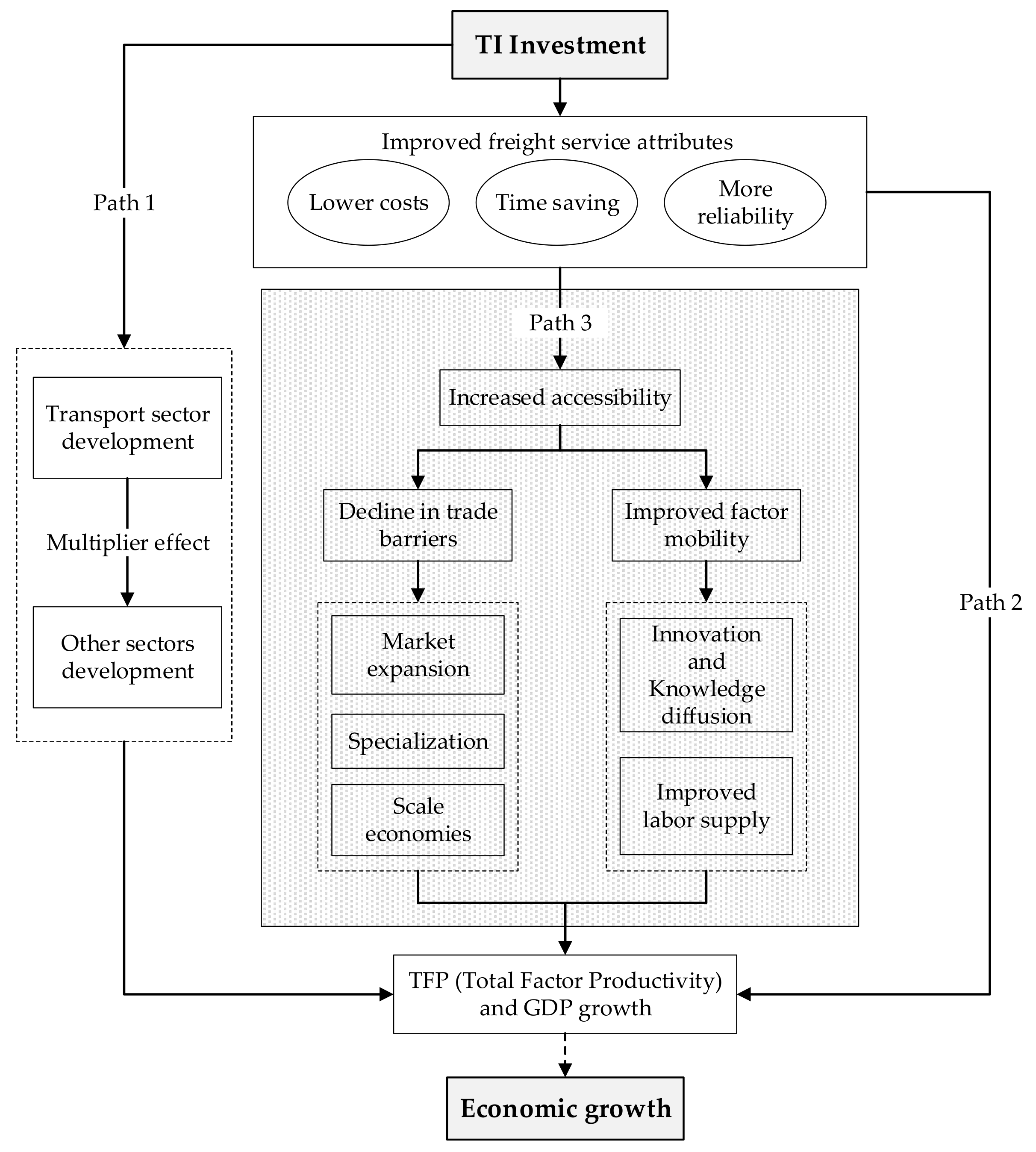
2.1. TI Investment and Economic Growth

TI investment has far-reaching impacts on economic activities, as revealed in the sectors of agriculture, manufacturing, and tourism [21,22,23]. A popular view highlights that TI investment contributes to economic growth [24]. Nevertheless, the evidence fully supporting such a view is doubted. In the US, TI investment relocated settlement and economic activities towards urban centers, aligning economic growth with the evolution of urbanization [25]. By contrast, TI investment’s positive impacts on economic growth have not yet been found extensively in the EU [7].

It is reasonable to assume that the relationship between TI investment and economic growth is not monotonic. TI investment generates a region’s economic vitality through inflowing capital and immigrants [10]. Thereby, poverty reduction, employment generation, and knowledge spillover can be realized for economic growth [7,20,26]. However, the role of TI investment in economic growth is often doubted. Canning and Pedroni [27] pinpointed that TI investment creates an economic burden if its size is larger than the optimal value. Mahmoudzadeh et al. [28] echoed that the increase of TI investment and the decrease of private sector investment forces economic growth to slow down. Upon these arguments, it seems that the contribution of TI investment to economic growth will not be substantial without accounting for regional conditions, economic development phases, and institutional factors [8,29].

Academia has offered three types of paths to elaborate the impacts of TI investment on economic growth; namely, multiplier effects, cost-saving effects, and wider economic impacts (WEI), as shown in Figure 1 [30]. As a capital input, TI investment demands construction-related sectors increase fiscal spending, and stimulates multiplier effects in economic development [31] The production process is reorganized over regions by improved transport services bringing benefits such as lower cost, saving time, and higher reliability [30]. The realization of cost-saving further accelerates the improvement of total factor productivity [32]. TI investment’s WEI, promoted by better accessibility, will unfurl over time [33]. The erosion of trade barriers resulting from TI investment helps enterprises explore abundant business opportunities [11]. Furthermore, the lowering of trade barriers facilitates enterprises to achieve specialization and scale economies in a wider region.

Another aspect of WEI lies in the advancement of factor mobility (i.g., capital, labor). For instance, the relaxation of capital flows concurs with the reconstruction of industrial structure to create commercial innovations and new technologies [34], providing a competitive business environment for small firms to survive. In addition, reducing travel time and costs enables people to move into other areas searching for business opportunities, increasing the availability of labor resources in different areas [20]. In this process, more frequent interaction and cooperation among people spurs disseminating specialized knowledge and new ideas [7]. Nonetheless, researchers also noted that these positive effects might not be converted into economic growth if the region lacks a “social filter” like socioeconomic and institutional conditions [7].

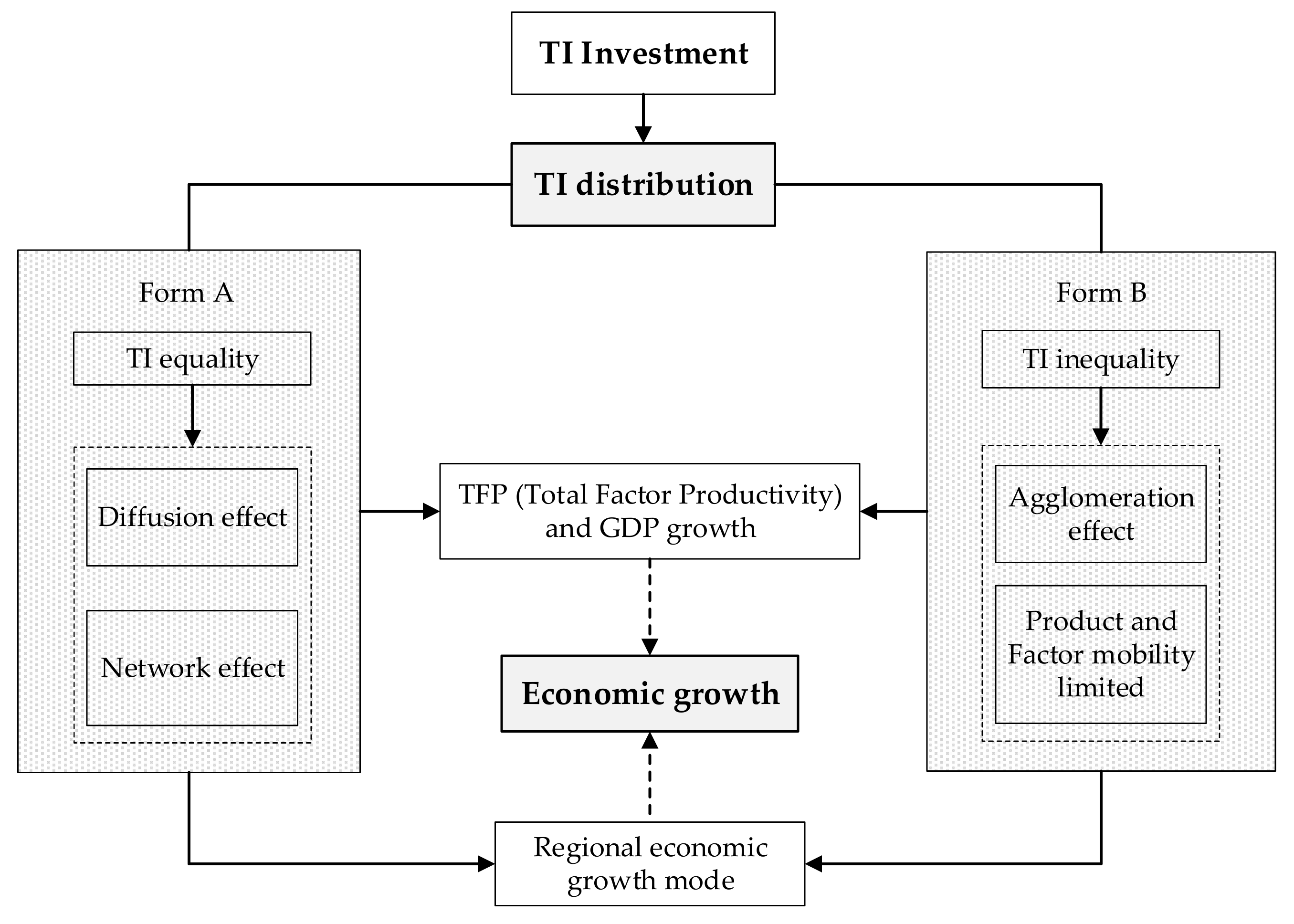
2.2. TI Distribution and Economic Growth

TI investment is instrumental in altering the status of TI distribution, as shown in Figure 2. On the one hand, TI equality advances the deployment of productivity across regions. Due to resource limits, however, many countries are subject to difficulty in embarking on large-scale TI investment once for all regions, as balanced growth theory claims. Especially in underdeveloped economies, TI equality makes regions face insufficient TI stocks, resulting in a low growth rate in national income. On the other hand, TI inequality underscores the part the regions play in taking the lead on economic growth, matching the principles of unbalanced growth theory. However, it does not imply that TI inequality is the only choice that regions have to accept. The widening economic growth gap caused by TI inequality may be treated as a deterrence to sustainable growth [35].

Agglomeration is an effect of TI inequality, encouraging a region to attract production factors from other places to develop the economy [31]. Some experts have inquired about such a pattern of growth [36], as it merely reflects the redistribution of production factors from one region to another. In Vickerman’s [33] opinion, this explains the acceleration of impacts in one region “at the expense of another” a landscape of gainers and losers. Despite the potentially disruptive impacts, scholars tend to treat agglomeration as bringing overall gains at the larger regional scale [33,37]. They concur on the negative impacts of excessive agglomeration, such as environmental pollution, traffic congestion, and intensive business competition [38,39], and account for the bell-shaped relationship between transport costs and agglomeration [40,41]. TI inequality also leads to negative impacts such as market vulnerability, interruption of knowledge spillover, and resource allocation inefficiency [42]. Thus, those agglomerated regions are important in changing TI inequality, focusing on evacuating enterprises, population, and obstacles to realize economic growth.

Network and diffusion effects are two other kinds of impacts caused by TI equality which deserve rethinking in academia. TI equality stands for a relatively realistic transport network in bringing convenience for producers to possess a unified and broader trading market [43] and increased trade opportunities to fortify economic integration [44]. A recent study by He et al. [45] clarified that the essence of a traffic network affecting economic integration depends on its improved mobility system for production factors. The importance of economic integration to economic growth has been a consensus in the literature. Economic integration spurs economic activity mainly in regional division and cooperation and growing trade [46,47]. Ricci [48] identifies the opposite on economic integration as benefits from agglomeration cannot be reaped, preventing regional disparities from growing.

The diffusion effect can be regarded as the economic stimulant influence of developed areas on the surrounding areas in a traffic network. In light of the diffusion effect, researchers have confirmed that the spatial interaction between TI distribution and economic activities laid a solid foundation for cultivating industrial traffic belts [12]. According to pole-axis theory, pole-axis exploitation’s impacts on economic growth are greater than that of isolated economic growth pole exploitation. The pole-axis exploitation effect facilitates the coordinated development of regional economies [49]. However, it is reasonable to question that TI equality may lead to the plunder of production factors in undeveloped regions [50].

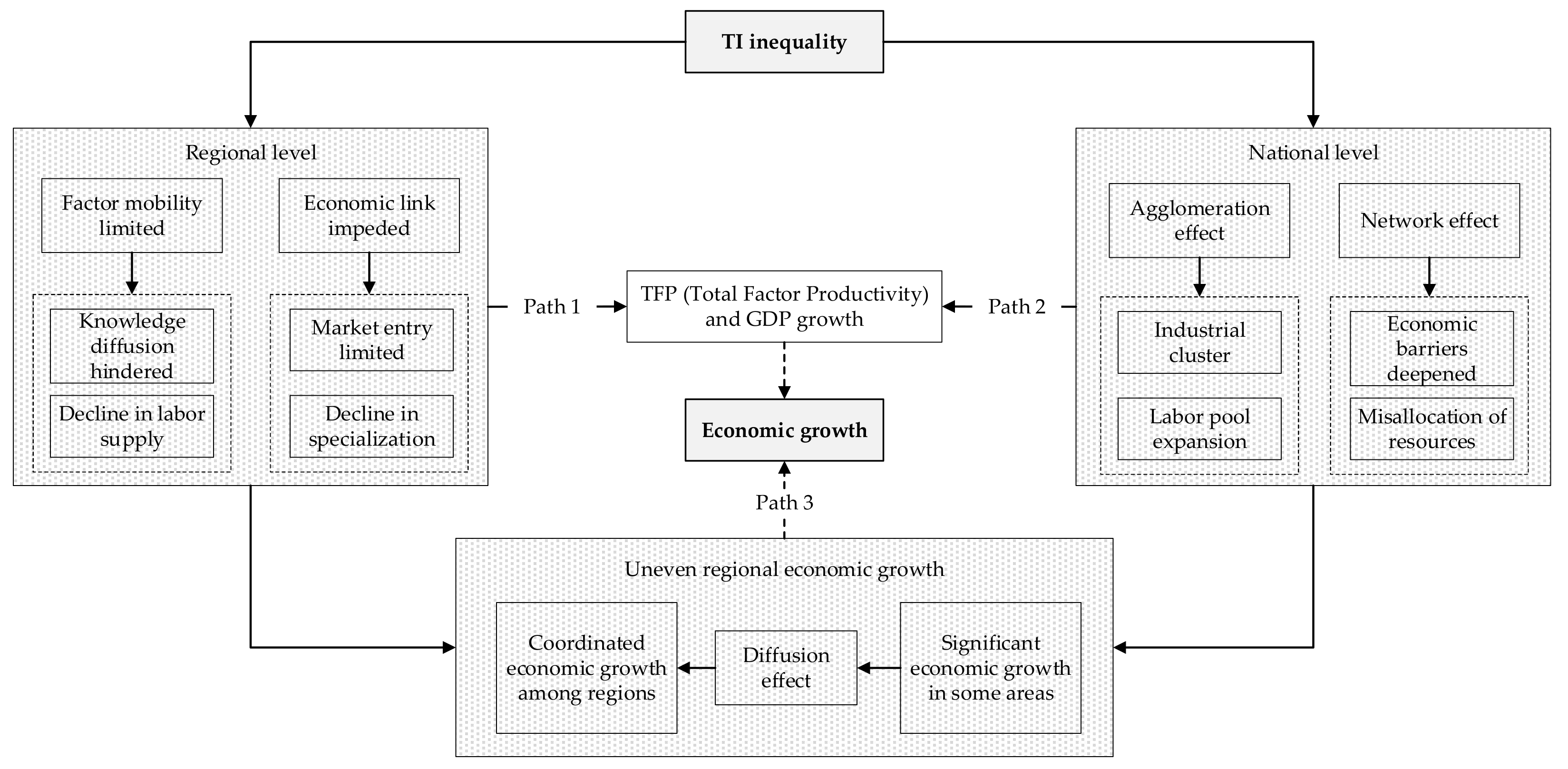
2.3. TI Inequality and Economic Growth

Inequality is common in the areas of income, education, health, and welfare [51,52,53]. In the field of transport, much attention has been directed to accessibility inequality. In a highly urbanized country, the situation is far from being spatially equitable in accessibility [54]. The opening of high-speed railways (HSR) may increase inequalities in the territorial connections [55]. The previous studies showed that the trend of inequality might depend on the dimensions. With the HSR network expanding, the disparity between economic regions or between megalopolises has reduced, while other cities not belonging to any major city cluster are further lagging behind [56]. The consequences of inequality caused by TI need to be considered seriously.

Despite this, equality may also be detrimental to development. Based on the premise that people have similar development potentials, opportunities should be equitably distributed. Regional economic vitality varies with resource endowment, social institutions, and geographical position. Probably, for this reason, spatial inequality usually produces different results from the perspective of human-centered inequality. Following the principle of equality in resource allocation will create more inequality among regions. Allocating the same TI resources to undeveloped areas as developed areas reduces efficiency and prevents undeveloped areas from developing [27,28]. Considering the importance of these issues, scholars in the inequality area have attempted to look at regional space [1]. As shown in Figure 3, researchers’ discussion over the impacts of TI inequality on economic growth revolves around three paths.

Path One: TI inequality impedes production factors from freely flowing. Increased commuting time and costs are unbeneficial to the increase of labor mobility. Therefore, enterprises have to search for human resources from a given geographical area, so the human resources supply chain might lag behind market demand (Jiwattanakulpaisarn et al., 2010). Another threat caused by limited migration is restricting opportunities to disseminate knowledge and technology [42]. Subject to TI inequality, capital investment occurs in some industries or regions, discouraging capital flow to innovation and industrial improvement [34]. Besides, uneven transport distribution reduces economic links among regions. Consequently, firms will not reap the benefits of specialization and scale of economies in a broader market [30].

Path Two: researchers argued that TI inequality helps those regions with relative transport advantages attract firms and households from other regions to establish an industrial cluster. Once an industrial cluster is shaped, firms can gain the advantages of the external economy through the tight connection between economic agents [57]. The increase in population expands the labor pool, which is conducive to matching workers with positions and learning from each other [7]. As detected by Cohen and Paul [58], these benefits from agglomeration ultimately reduce costs and improve production efficiency. Nevertheless, the existence of TI inequality weakens the efficiency of transport networks. As a result, less-developed regions have to bear relatively high transport costs and trade barriers, which are unhelpful in optimizing production resource deployment in a larger scope [19,59].

Path Three: it is inferred that TI inequality at both national and regional levels causes uneven economic growth in the long run. Due to agglomeration, economic growth can bounce in some regions. With the improvement of transport, the diffusion effect will be surfacing. A typical case is that developed areas tend to transfer advanced knowledge and technologies to undeveloped areas. Consequently, the accomplishment of coordinated economic growth becomes possible among regions. The diffusion effect shall be impeded if TI is not distributed equally. Such a process is called Path 3. TI inequality causes an economic development gap among regions, having negative impacts on long-term economic growth.

3. Case Study

Given homogeneity and comparability of data between provinces, we selected China to evaluate the impacts of TI inequality on economic growth [11,50]. As revealed in previous studies [11], China has accumulated much experience resolving the problem of TI, offering a valuable reference to other developing countries. China is one of the hugest countries in the world. It is necessary to group those adjacent areas with similar geographical conditions and resource endowment into several regions. In China, eastern, central, and western areas are often cited [60,61] regarding distance or per capita GDP comparisons [62]. While such regional groupings cannot show the tiny differences between regions, we followed the Development Research Center of the Central Government (2005) to separate the whole of China into eight regions, as shown in Figure 4. This eight-region classification initiative is suitable for a study based on internal similarity and inter-regional attributes.

Since the late 1980s, China’s economy has undergone dramatic changes. As

Table 1. Profiles of eight regions of China.

Index	Year	NER	NCR	ECR	SCR	MYL	MYT	SWR	NWR
Average GDP per capita (CNY)	81–85	866	1239	1551	615	528	503	397	576
	86–90	1750	2324	2826	1458	1062	1013	807	1107
	91–95	3867	5348	7276	4291	2277	2167	1967	2304
	96–00	7659	12,044	15,735	8799	4806	4589	4127	4510
	01–05	12,106	21,908	26,538	14,060	8872	7687	6451	7737
	06–10	25,343	43,699	49,309	28,237	23,034	17,164	14,441	16,421
	11–15	47,646	71,500	78,402	50,679	44,054	35,550	30,661	32,230
Average annual GDP per capita growth rate	81–85	11.38%	11.57%	9.76%	16.10%	14.29%	13.42%	12.26%	12.20%
	86–90	14.12%	12.56%	11.20%	18.65%	13.50%	13.76%	16.07%	12.73%
	91–95	20.96%	22.90%	27.85%	27.42%	20.59%	20.78%	23.00%	18.56%
	96–00	9.90%	12.44%	9.77%	9.35%	10.34%	10.44%	8.95%	10.11%
	01–05	11.78%	14.73%	13.73%	12.06%	17.68%	13.39%	13.04%	13.46%
	06–10	16.59%	13.17%	11.42%	14.80%	20.03%	18.61%	17.77%	16.88%
	11–15	9.06%	8.04%	8.33%	10.18%	9.01%	11.88%	13.33%	10.86%

Source: National Bureau of Statistics of China.

illustrates, most of the eight regions had an annual economic growth rate of more than 10% during the analyzed period. Due to geographical advantages and market accessibility, the coastal areas had attracted a larger amount of foreign investment and trade than the inland areas to grow economies [19]. The resulting widening economic gaps between the coastal and inland areas posed a challenge to China regarding sustainable development [50]. Several milestone strategies have thus been implemented, such as the West Development Strategy (WDS), the Rising of the Central Regions Strategy (RCRS), and the Revitalizing Northeast Old Industrial Base (RNOIB). Whereas inland regions maintained faster economic growth than before, they are still subject to smaller per capita GDP than coastal areas. Therefore, increasing the public budget for TI investment in undeveloped regions is key to China’s national strategies.

In China, most passenger and freight traffic is reliant on highways and railways. According to the China Statistical Yearbook, the passenger traffic of railway and highway transport occupies more than 90% of the whole. Likewise, the share of railway and highway transport in freight traffic remains more than 80%. China has been engaged in building a nationwide transport network [50]. For instance, the total length of railways and highways had surged several times over the past decades, as shown in

Table 2. Length of China’s TI from 1980 to 2015 (10,000 km).

Year	Railways in Operation	Highways	Expressway	Navigable Inland Waterways	Regular Civil Aviation Routes
1980	5.33	88.83	0	10.85	19.53
1985	5.52	94.24	0	10.91	27.72
1990	5.79	102.83	0.05	10.92	50.68
1995	6.24	115.70	0.21	11.06	112.90
2000	6.87	167.98	1.63	11.93	150.29
2005	7.54	334.52	4.10	12.33	199.85
2010	9.12	400.82	7.41	12.42	276.51
2015	12.10	457.73	12.35	12.70	531.72

Unit: 10,000 km.

. Despite this, TI inequality problems have spread nationwide (see

Table 3. Regional TI density in China.

Index	Year	NER	NCR	ECR	SCR	MYL	MYT	SWR	NWR
Density of Railways in Operation	1982	152.85	149.43	84.87	55.89	60.58	105.32	55.36	11.36
	1985	152.81	162.94	84.87	57.98	63.16	107.55	55.76	12.31
	1990	152.63	175.15	88.93	57.26	66.27	111.01	55.91	12.27
	1995	152.15	183.96	92.03	57.47	67.77	116.04	57.31	13.25
	2000	152.82	208.48	85.69	53.29	70.56	123.47	62.24	15.58
	2005	169.88	264.10	150.64	121.09	97.14	155.23	82.94	16.81
	2010	178.76	289.52	195.27	164.99	123.02	193.89	92.90	24.97
	2015	216.47	398.30	272.76	246.63	157.87	253.50	126.72	34.23
Density of Highways	1982	1253	2354	2067	2892	802	2218	1393	185
	1985	1304	2416	2273	2984	805	2270	1470	189
	1990	1444	2653	2673	3238	907	2389	1627	206
	1995	1568	3299	3029	4353	980	2526	1783	221
	2000	1663	4123	3515	5102	1351	2844	2334	249
	2005	2169	4912	6612	5809	1651	4464	3160	420
	2010	4364	11,368	12,919	9019	3985	10,281	6223	863
	2015	4833	13,161	13,751	10,363	4305	11,832	7333	1034

Source: National Bureau of Statistics of China. The unit of density is a kilometer per 10,000 km².

). In the past planned economy, most transport investments were made to coastal regions [14]. NCR, ECR, and SCR won more TI resources than other regions. Consequently, TI inequality between the coastal and inland areas was widening. Although a series of regional balancing programs (e.g., WDS, RCRS, and RNOIB) had been in place, the benefits were fewer than anticipated [63].

4. Methodology

4.1. Indicators and Data

Data were collected from the China Statistical Yearbook (1983–2016) and China Statistical Yearbook for Regional Economies (2000–2014). Given their dominance in delivering transport services, we examined both highways and railways to present TI development in the country. The indicator of investment was used to represent the development of the transport sector [13]. Physical measurements (e.g., density, length) were considered better than financial measures (e.g., government investment) to describe the development of transport infrastructure [32]. Considering that physical measurements do not need data about transport investment of private sectors, which are often unavailable, we employed mileage per capita to quantify transport distribution differences. Mileage per capita, which could reflect construction costs and actual demand of TI, is more appropriate for evaluating the difference in TI distribution [2]. In China, the direct comparison between coastal and inland provinces by the indicators of total mileage or network density would almost be meaningless.

Highways and railways are two of the most fundamental means of transportation, but they devote different values to economic growth [64]. The impacts of highways on economic growth might be more substantial than those of railways, but limits to ‘returns of scale’ can be formed by the accessibility of highway networks [65]. In reverse, the increase of railway accessibility enhances the marginal outputs related to the rise in highway accessibility [65]. Given the differences and linkage between railways and highways, weightings are quantified using the following Equation:

$$a{t}_{i,t}={\omega }_{H,t}\times \frac{Highwa{y}_{i,t}}{Populatio{n}_{i,t}}+{\omega }_{R,t}\times \frac{Railwa{y}_{i,t}}{Populatio{n}_{i,t}}$$

(1)

where $i$ and $t$ represent province $i$ and year $t$, and $a{t}_{i,t}$ denotes the weighted mileages per capita. $Highwa{y}_{i,t}$ and $Railwa{y}_{i,t}$ indicate the lengths of highway and railways, respectively. $Populatio{n}_{i,t}$ refers to the population of province i in year t. ${\omega }_{R,t}$ and ${\omega }_{H,t}$ represent the percentages of railway transport volume and highway transport volume, respectively. ${\omega }_{R,t}+{\omega }_{H,t}=1$.

GDP per capita is a yardstick to quantify regional economic growth [66]. In addition, it reflects the quality of life indirectly. Therefore, GDP per capita is employed to quantify economic growth. Chongqing was incorporated in Sichuan province for better coherence and continuity of the data as it was promoted to be a municipality in 1997. Similarly, Hainan was included in Guangdong province. On the other hand, Qinghai and Tibet were excluded due to their characteristics and inadequate datasets.

4.2. TI Inequality Measures

The Theil index and the Gini coefficient are the two most popular methods for quantifying inequality [67]. The larger the Theil index, the greater the inequality. In a similar vein, the higher the Gini coefficient is, the more unequal the object’s distribution is across the population. The Gini coefficient method creates a whole picture of inequality and reveals the share of each region using the decomposition of the Gini coefficient [2,53]. Therefore, the Gini coefficient method is selected to quantify the degree of TI inequality in the study.

The weighted mileage per capita per province is adopted to calculate the Gini coefficient, as Equation (2) indicates. In this equation, $\mathrm{G}$ denotes the Gini coefficient, and $n_i$ and $n_j$ refer to the populations of provinces $i$ and j, respectively. $N={\displaystyle \sum }_i{n}_i$; $u$ means the weighted average mileage per capita of the study area; $a{t}_i$ and $a{t}_j$ represent weighted mileage per capita in provinces $i$ and $j$, respectively.

$$G=\frac{1}{2N^{2}u}{\displaystyle \sum }_i{\displaystyle \sum }_j{n}_i{n}_j|a{t}_i-a{t}_j|$$

(2)

Equation (2) is further rewritten below to dig out the contribution of each region [68,69]. In Equation (3), ${\chi }_{ij}$ denotes the relative deprivation between provinces $i$ and $j$, and ${\chi }_{ij}=max|n_i{n}_j\left(a{t}_i-a{t}_j\right),0|$; providing that the study area contains $\mathrm{m}$ regions, $N_s$ and $u_s$ represent population and average weighted mileage per capita in region $\mathrm{s}$. ${\theta }_s=\frac{N_s}{N}$, ${\gamma }_s=\frac{u_s}{u}$.

$$G=\frac{1}{2N^{2}u}{\displaystyle \sum }_i{\displaystyle \sum }_j{n}_i{n}_j|a{t}_i-a{t}_j|=\frac{1}{N^{2}u}{\displaystyle \sum }_i{\displaystyle \sum }_j{\chi }_{ij}$$

(3)

Equations (4) and (5) are proposed in line with Hong’s propositions [70], where $G_s$ denotes the Gini coefficient of region $s$, $G_{-s}$ is the relative deprivation per capita between region $\mathrm{s}$ and the remainder; ${\theta }_s^2{\gamma }_s{G}_s∕G$ and $\left({\theta }_s-{\theta }_s^2\right){\gamma }_s{G}_{-s}∕G$ represent the contribution rate of internal and external disparities in a region $\mathrm{s}$ to the absolute difference, respectively.

$$G=\frac{1}{N^{2}u}{\displaystyle \sum }_i{\chi }_i=\frac{1}{N^{2}u}{\displaystyle \sum }_s^m{\displaystyle \sum }_{iϵs}\left({\displaystyle \sum }_{jϵs}{\chi }_{ij}+{\displaystyle \sum }_{j\notin s}{\chi }_{ij}\right)={\displaystyle \sum }_s^m{\theta }_s^2{\gamma }_s{G}_s+{\displaystyle \sum }_s^m\left({\theta }_s-{\theta }_s^2\right){\gamma }_s{G}_{-s}$$

(4)

$$G_{-s}=\frac{1}{N_s\left(N-N_s\right)u_s}{\displaystyle \sum }_{iϵs}{\displaystyle \sum }_{j\notin s}{\chi }_{ij}$$

(5)

Concerning the subgroup decomposition equations, the approach proposed by Mookherjee and Shorrocks is adopted (see Equation (6)) [53]. In the equation, $G_b$ denotes the Gini coefficient of inter-regional TI disparities, ${\displaystyle \sum }_s{\theta }_s^2{\gamma }_s{G}_s$ represents internal TI disparities; $R$ denotes the residual term, which reflects the interaction effect and overlapping between regions [71].

$$\begin{gathered} G={\displaystyle \sum }_s{\theta }_s^2{\gamma }_s{G}_s+\frac{1}{2}{\displaystyle \sum }_s{\displaystyle \sum }_k{\theta }_k{\theta }_s|{\gamma }_s-{\gamma }_k|+R \\ ={\displaystyle \sum }_s{\theta }_s^2{\gamma }_s{G}_s+G_b+R \end{gathered}$$

(6)

4.3. Granger Causality Analysis

Granger [72] developed a model test method, namely the Granger causality test, to detect the causal relationship between two variables. The Granger causality test determines whether the lagged value of a variable can be introduced to the equation of other variables. If the past information about X explains much about the present Y, then there is a one-way causality from X to Y. In reverse, if the past Y has a significant effect on the current X, then the inverse single causal relationship also exists. The causal relationship between X and Y should be bidirectional if the causality is found true in both directions.

In this paper, the Granger causality analysis is used to test the causality between economic growth and TI inequality at both the national and sub-national levels. Two initial steps were implemented: panel unit root tests and cointegration tests. The panel unit root tests aim to determine whether the variables are stationary. The ADF test is conducted to eliminate the white noise characteristics of stochastic errors. If the original series fail to pass the unit root test, the differential method may reduce the stochastic trend, namely the stationary difference process. In the second step, the panel cointegration test is intended to examine whether the linear combination of variables is a stationary series and whether the causal relationship described by the regression equation is a spurious regression. Cointegration tests can be divided into two types: one is based on the regression coefficient (e.g., Johansen test); the other is based on the regression residual (e.g., CRDW test, EG test, AEG test).

5. Result of the Data Analysis

5.1. Trends of TI Inequality

The national and regional Gini coefficients were calculated using Equation (3). The results are listed in

Table A1. National, regional, and inter-regional Gini coefficients.

Year	NER	NCR	ECR	SCR	MYL	MYT	SWR	NWR	Inter-Regional	National
1982	0.1163	0.1258	0.1502	0.0479	0.2833	0.1198	0.0945	0.0070	0.1621	0.2352
1983	0.1180	0.1251	0.1504	0.0504	0.2820	0.1177	0.0909	0.0104	0.1609	0.2334
1984	0.1126	0.1261	0.1557	0.0526	0.2799	0.1147	0.0844	0.0095	0.1592	0.2300
1985	0.1007	0.1244	0.1630	0.0579	0.2797	0.1121	0.0909	0.0065	0.1601	0.2271
1986	0.0872	0.1259	0.1632	0.0602	0.2832	0.1078	0.0900	0.0066	0.1581	0.2271
1987	0.0751	0.1211	0.1625	0.0636	0.2876	0.1063	0.0869	0.0214	0.1603	0.2269
1988	0.0712	0.1166	0.1693	0.0278	0.2864	0.1053	0.0893	0.0272	0.1700	0.2314
1989	0.0707	0.1194	0.1720	0.0306	0.2849	0.0971	0.0935	0.0242	0.1667	0.2284
1990	0.0657	0.1169	0.1844	0.0759	0.2804	0.1007	0.0978	0.0237	0.1589	0.2243
1991	0.0643	0.1231	0.1866	0.0779	0.2763	0.1004	0.1009	0.0234	0.1564	0.2222
1992	0.0594	0.1265	0.1839	0.0770	0.2731	0.1017	0.1039	0.0242	0.1532	0.2194
1993	0.0588	0.1223	0.1968	0.0681	0.2662	0.1029	0.1082	0.0384	0.1525	0.2180
1994	0.0534	0.1086	0.2004	0.0337	0.2620	0.1038	0.1120	0.0424	0.1569	0.2193
1995	0.0514	0.0896	0.2086	0.0201	0.2550	0.0852	0.1150	0.0566	0.1594	0.2174
1996	0.0501	0.0870	0.2079	0.0138	0.2546	0.0814	0.1191	0.0647	0.1570	0.2158
1997	0.0513	0.0879	0.2100	0.0121	0.2652	0.0773	0.1271	0.0651	0.1542	0.2171
1998	0.0493	0.0754	0.2218	0.0102	0.2882	0.0697	0.1304	0.0674	0.1486	0.2181
1999	0.0469	0.0491	0.2278	0.0161	0.2962	0.0679	0.1778	0.0698	0.1483	0.2282
2000	0.0456	0.0404	0.2306	0.0334	0.2943	0.0657	0.1833	0.0447	0.1443	0.2246
2001	0.0915	0.0506	0.0960	0.0338	0.2884	0.0950	0.2644	0.2434	0.1520	0.2420
2002	0.0850	0.0427	0.0999	0.0303	0.2884	0.0678	0.2363	0.2440	0.1500	0.2331
2003	0.0827	0.0411	0.0863	0.0315	0.2888	0.0665	0.2313	0.2421	0.1461	0.2297
2004	0.0783	0.0496	0.0866	0.0361	0.2895	0.0649	0.2286	0.2446	0.1389	0.2238
2005	0.0845	0.0609	0.0941	0.0376	0.2799	0.0583	0.2124	0.2427	0.1394	0.2180
2006	0.1069	0.0683	0.1140	0.0480	0.1344	0.0585	0.1550	0.1651	0.1363	0.1842
2007	0.1101	0.0761	0.1147	0.0475	0.1472	0.0591	0.1448	0.1524	0.1409	0.1877
2008	0.1199	0.0888	0.1148	0.0524	0.1591	0.0612	0.1291	0.1423	0.1461	0.1932
2009	0.1220	0.0914	0.1191	0.0541	0.1667	0.0679	0.1297	0.1317	0.1529	0.2016
2010	0.1228	0.0974	0.1148	0.0550	0.1699	0.0715	0.1186	0.1242	0.1582	0.2074
2011	0.1233	0.1011	0.1174	0.0555	0.1717	0.0747	0.1168	0.1131	0.1631	0.2119
2012	0.1252	0.1093	0.1185	0.0556	0.1770	0.0612	0.1168	0.1129	0.1663	0.2150
2013	0.1158	0.1088	0.1207	0.0579	0.1821	0.0601	0.1185	0.1079	0.1651	0.2137
2014	0.1104	0.1122	0.1204	0.0518	0.1872	0.0677	0.1204	0.1003	0.1666	0.2156
2015	0.1028	0.1112	0.1195	0.0552	0.1914	0.0689	0.1207	0.0914	0.1678	0.2177

(Appendix A). Two curves were graphed to exhibit TI’s national and regional inequality. As Figure 5 shows, the national TI inequality had seemingly experienced four periods of development. During the first period (1982–1996), the Gini coefficient gradually declined from 0.2352 to 0.2158. The second period was from 1996 to 2001, characterized by the coefficient’s increase by more than 12%. The third one refers to the period from 2001 to 2006, during which the coefficient dropped dramatically to the lowest point of 0.1842. Last, the coefficient has been mounting by the year 2015. Regarding the inter-regional TI inequality, the tendency is very similar to the trajectory of the national Gini coefficient. For simplicity, the intra-regional curve is not described here.

To explore the composition of national TI inequality, we further calculated the intra- and inter-regional contributions to the Gini coefficient based on Equation (6) (see

Table A2. The contribution rate of intra-regional, inter-regional and residual term.

Year	Intra-Regional	Inter-Regional	Residual Term	Year	Intra-Regional	Inter-Regional	Residual Term
1982	0.0810	0.6891	0.2299	1999	0.0892	0.6501	0.2608
1983	0.0806	0.6894	0.2300	2000	0.0904	0.6422	0.2675
1984	0.0800	0.6920	0.2281	2001	0.1013	0.6280	0.2706
1985	0.0810	0.7050	0.2139	2002	0.0955	0.6433	0.2612
1986	0.0808	0.6965	0.2227	2003	0.0951	0.6363	0.2686
1987	0.0797	0.7063	0.2140	2004	0.0966	0.6209	0.2825
1988	0.0757	0.7345	0.1898	2005	0.0949	0.6396	0.2655
1989	0.0767	0.7302	0.1932	2006	0.0810	0.7401	0.1789
1990	0.0818	0.7084	0.2098	2007	0.0804	0.7504	0.1692
1991	0.0832	0.7042	0.2126	2008	0.0789	0.7563	0.1648
1992	0.0847	0.6984	0.2169	2009	0.0783	0.7585	0.1632
1993	0.0850	0.6994	0.2156	2010	0.0748	0.7628	0.1624
1994	0.0814	0.7155	0.2031	2011	0.0738	0.7700	0.1561
1995	0.0769	0.7330	0.1900	2012	0.0719	0.7737	0.1544
1996	0.0772	0.7277	0.1950	2013	0.0727	0.7722	0.1551
1997	0.0803	0.7100	0.2096	2014	0.0737	0.7730	0.1534
1998	0.0828	0.6814	0.2358	2015	0.0732	0.7708	0.1560

). The results displayed in Figure 6 indicate that the inter-regional TI inequality occupies an average of more than 70% of the total difference, and the intra-regional contribution maintains between 7.19% and 10.13%. It is found that the national inequality in TI mostly comes from the inter-regional disparity of each region. Not surprisingly, these findings demonstrate the validity and rationality of the previous regional classifications. Among these regions, SWR, MYL, MYT, and NWR contributed significantly to the total difference, as shown in

Table A3. The contribution rate of external disparities of each region to the overall inequality.

Year	NER	NCR	ECR	SCR	MYL	MYT	SWR	NWR
1982	0.1444	0.0284	0.0016	0.1270	0.1762	0.1166	0.1828	0.1421
1983	0.1379	0.0277	0.0020	0.1297	0.1750	0.1165	0.1856	0.1451
1984	0.1391	0.0270	0.0028	0.1292	0.1767	0.1145	0.1871	0.1436
1985	0.1424	0.0264	0.0034	0.1307	0.1620	0.1117	0.1991	0.1433
1986	0.1418	0.0256	0.0041	0.1297	0.1799	0.1074	0.1918	0.1388
1987	0.1410	0.0235	0.0051	0.1280	0.1781	0.1030	0.1916	0.1500
1988	0.1399	0.0226	0.0055	0.1638	0.1666	0.0941	0.1896	0.1421
1989	0.1348	0.0233	0.0060	0.1657	0.1654	0.0919	0.1958	0.1405
1990	0.1482	0.0236	0.0072	0.1225	0.1712	0.0925	0.2106	0.1423
1991	0.1474	0.0263	0.0075	0.1228	0.1701	0.0885	0.2134	0.1406
1992	0.1506	0.0286	0.0081	0.1201	0.1676	0.0857	0.2156	0.1389
1993	0.1457	0.0314	0.0091	0.1348	0.1609	0.0782	0.2146	0.1403
1994	0.1411	0.0343	0.0087	0.1724	0.1522	0.0714	0.2065	0.1321
1995	0.1391	0.0327	0.0077	0.1976	0.1485	0.0679	0.1994	0.1300
1996	0.1344	0.0356	0.0075	0.2044	0.1514	0.0637	0.1967	0.1291
1997	0.1276	0.0349	0.0068	0.1952	0.1788	0.0577	0.1969	0.1217
1998	0.1160	0.0351	0.0072	0.1828	0.2040	0.0540	0.2035	0.1146
1999	0.0999	0.0347	0.0064	0.1675	0.2037	0.0452	0.2505	0.1029
2000	0.0938	0.0317	0.0047	0.1418	0.2117	0.0500	0.2666	0.1093
2001	0.0811	0.0107	0.0043	0.0874	0.1419	0.1007	0.2953	0.1773
2002	0.0771	0.0102	0.0041	0.0812	0.1451	0.1111	0.2985	0.1774
2003	0.0842	0.0100	0.0048	0.0766	0.1541	0.1077	0.2922	0.1751
2004	0.0898	0.0095	0.0088	0.0696	0.1598	0.1034	0.2836	0.1789
2005	0.0896	0.0092	0.0087	0.0672	0.1673	0.0990	0.2843	0.1797
2006	0.1081	0.0249	0.0023	0.0187	0.2173	0.1604	0.1852	0.2021
2007	0.0991	0.0250	0.0030	0.0165	0.2267	0.1482	0.2066	0.1944
2008	0.1012	0.0247	0.0039	0.0147	0.2268	0.1421	0.2244	0.1833
2009	0.0911	0.0251	0.0041	0.0133	0.2224	0.1424	0.2431	0.1803
2010	0.0827	0.0224	0.0047	0.0130	0.2135	0.1628	0.2544	0.1717
2011	0.0820	0.0218	0.0049	0.0127	0.2097	0.1623	0.2628	0.1699
2012	0.0793	0.0240	0.0048	0.0126	0.2053	0.1639	0.2596	0.1786
2013	0.0779	0.0260	0.0045	0.0138	0.2004	0.1639	0.2618	0.1791
2014	0.0777	0.0256	0.0042	0.0142	0.1940	0.1614	0.2675	0.1818
2015	0.0769	0.0259	0.0042	0.0146	0.1871	0.1679	0.2738	0.1766

. Considering that this study is mainly concerned with the impact of TI inequality on economic growth, the calculation results of TI inequality will not be discussed in-depth. More empirical evidence about TI inequality can be found in Appendix A.

5.2. Values of the Granger Causality Test

5.2.1. Panel Unit Root Tests

The data of GDP per capita was deflated by price indices based on the constant price of 1982. Then, a logarithm was adopted for all variables to eliminate heteroskedasticity in the time series. After this process, X was denoted as LNX. Finally, the unit root tests were conducted, and results were reported in

Table 4. Results of panel unit root test for China.

Variables	T-Statistic	Test Critical Values			Test Results
		1% Level	5% Level	10% Level
LN GDP per capita	0.2130	−3.6617	−2.9604	−2.6192	Non-stationary
LN Gini	−2.0163	−3.6463	−2.9540	−2.6158	Non-stationary
DLN GDP per capita	−4.2575	−3.6617	−2.9604	−2.6192	Stationary
DLN Gini	−5.1610	−3.6537	−2.9571	−2.6174	Stationary

,

Table 5. Results of panel unit root tests for various regions.

Region	Variables	t-Statistic	Test Critical Values			Test Results
			1% Level	5% Level	10% Level
NER	LN XLN	1.3609	−3.6617	−2.9604	−2.6192	N-S
	LN Y	−1.3423	−3.6463	−2.9540	−2.6158	N-S
	DLN X	−3.3933	−3.6617	−2.9604	−2.6192	S
	DLN Y	−5.2417	−3.6537	−2.9571	−2.6174	S
NCR	LN X	0.5232	−3.6617	−2.9604	−2.6192	N-S
	LN Y	−2.0774	−3.6702	−2.9640	−2.6210	N-S
	DLN X	−4.2549	−3.6617	−2.9604	−2.6192	S
	DLN Y	−3.6975	−3.6537	−2.9571	−2.6174	S
ECR	LN X	−3.5384	−3.7241	−2.9862	−2.6326	S
	LN Y	−1.4893	−3.6463	−2.9540	−2.6158	N-S
	DLN X	−3.5155	−3.6892	−2.9719	−2.6251	S
	DLN Y	−5.6792	−3.6537	−2.9571	−2.6174	S
SCR	LN X	−1.7943	−3.6537	−2.9571	−2.6174	N-S
	LN Y	−2.5410	−3.6537	−2.9571	−2.6174	N-S
	DLN X	−3.4223	−3.6537	−2.9571	−2.6174	S
	DLN Y	−4.0468	−3.6537	−2.9571	−2.6174	S
MYL	LN X	0.6064	−3.6537	−2.9571	−2.6174	N-S
	LN Y	−1.4890	−3.6463	−2.9540	−2.6158	N-S
	DLN X	−2.8692	−3.6617	−2.9604	−2.6192	S
	DLN Y	−5.7251	−3.6537	−2.9571	−2.6174	S
MYT	LN X	1.6019	−3.6617	−2.9604	−2.6192	N-S
	LN Y	−1.7438	−3.6463	−2.9540	−2.6158	N-S
	DLN X	−3.0658	−3.6617	−2.9604	−2.6192	S
	DLN Y	−7.3149	−3.6537	−2.9571	−2.6174	S
SWR	LN X	0.7367	−3.6537	−2.9571	−2.6174	N-S
	LN Y	−2.2785	−3.6617	−2.9604	−2.6192	N-S
	DLN X	−2.2922	−3.6537	−2.9571	−2.6174	N-S
	D LN Y	−2.2385	−3.6617	−2.9604	−2.6192	N-S
	DDLN X	−5.5125	−3.6617	−2.9604	−2.6192	S
	DDLN Y	−12.5963	−3.6617	−2.9604	−2.6192	S
NWR	LN X	0.6380	−3.6537	−2.9571	−2.6174	N-S
	LN Y	−1.8947	−3.6463	−2.9540	−2.6158	N-S
	DLN X	−3.1207	−3.6617	−2.9604	−2.6192	S
	DLN Y	−6.0670	−3.6537	−2.9571	−2.6174	S

Note: X represents GDP per capita; Y represents TI Gini coefficient; N-S represents non-stationary; S represents stationary.

. According to Table 4, neither LN GDP per capita nor LN TI inequality passed the unit root test at 10% or lower levels, which corresponds with the practical situation.

If the time series cannot pass the unit root test, the differential method can be adopted to reduce the stochastic trend. For simplicity, the first difference of X is denoted as DX, the second difference of X is denoted as DDX. Both variables turned into stationary series at 1% level through the first difference, which indicates that the time series are I(1).

In Table 5, almost all the regional original values of LN GDP per capita and LN TI Gini coefficient were tested to be non-stationary series, apart from ECR’s LN GDP per capita, which rejected the null hypothesis unit root test at 5% level. Thus, ECR will not be involved in the panel cointegration test for not meeting the prerequisites that only the same orders might be cointegrated. In addition, all regions except SWR were examined to have no unit root at the 10% level using the first difference between the two variables. As both first difference variables of SWR failed to pass the test, we further performed a second difference to the variables. The results showed that each variable of second-order difference is examined to be I(2).

5.2.2. Panel Cointegration Tests

Considering that only two variables are examined in cointegration tests and the series are I(1), we conducted the EG two-step test. As listed in

Table 6. Results of the panel cointegration test.

Region	Variables	T-Statistic	Test Critical Values			Cointegra-Ted or Not
			1% Level	5% Level	10% Level
National	et	−2.1714	−2.6369	−1.9513	−1.6107	YES
NER		−2.0824	−2.6369	−1.9513	−1.6107	YES
NCR		−2.1574	−2.6443	−1.9525	−1.6102	YES
SCR		−2.5639	−2.6392	−1.9517	−1.6106	YES
MYL		−2.5824	−2.6369	−1.9513	−1.6107	YES
MYT		−2.6609	−2.6369	−1.9513	−1.6107	YES
SWR		−2.3068	−2.64179	−1.9521	−1.6104	YES
NWR		−1.5687	−2.63690	−1.9513	−1.6107	NO

, most residuals (except NWR’s $e_t$) passed the unit root test. The results show a long-run equilibrium relationship between TI inequality and economic growth. Therefore, it is considered that the two variables of GDP per capita and the Gini coefficient have at least unidirectional Granger causality in the long run.

5.2.3. Granger Tests of Causality

The original values of LN GDP per capita and LN Gini coefficient that failed to pass the unit root tests cannot be used to detect the causal relationship. However, both variables’ first- or second-order difference had no unit roots at the 10% level or below, which means that variables through difference are all stationary series. Although the first- or second-order difference can eliminate possible trend factors of variables and solve multiple colinear problems in models, the long-term economic information of variables was excluded. Consequently, the first- or second-order difference variables were used to model the short-term relationship. In light of this, the Granger causality test was performed, and the results are shown in

Table 7. Results of the Granger causality test.

Region	Null Hypothesis	Lags
		1	2	3	4
National	DLN Y → DLN X	3.5262 * (0.0705)	1.7417 (0.1950)	1.8218 (0.1713)	1.7620 (0.1762)
	DLN X → DLN Y	0.0206 (0.8868)	0.1153 (0.8915)	0.0776 (0.9715)	0.2105 (0.9295)
NER	DLN Y → DLN X	0.7148 (0.4048)	0.9791 (0.3891)	1.6584 (0.2037)	1.3410 (0.2894)
	DLN X → DLN Y	0.4675 (0.4996)	0.4133 (0.6657)	0.4179 (0.7419)	0.1432 (0.9639)
NCR	DLN Y → DLN X	0.1855 (0.6699)	0.0770 (0.9261)	0.0961 (0.9614)	0.3607 (0.8336)
	DLN X → DLN Y	0.0262 (0.8726)	0.0440 (0.9570)	0.0818 (0.9693)	0.0976 (0.9820)
ECR	DLN Y → DLN X	0.0964 (0.7584)	0.0123 (0.9878)	0.0747 (0.9730)	0.0178 (0.9993)
	DLN X → DLN Y	1.0046 (0.3245)	0.4900 (0.6182)	0.3150 (0.8144)	0.1907 (0.9405)
SCR	DLN Y → DLN X	3.4184 * (0.0747)	2.9420 * (0.0705)	2.0866 (0.1298)	1.5555 (0.2247)
	DLN X → DLN Y	5.3792 ** (0.0276)	2.2710 (0.1233)	3.2121 ** (0.0418)	3.4599 ** (0.0265)
MYL	DLN Y → DLN X	1.5690 (0.2204)	1.2069 (0.3154)	1.0066 (0.4077)	1.1755 (0.3515)
	DLN X → DLN Y	2.0416 (0.1637)	1.6915 (0.2039)	1.1275 (0.3586)	0.9727 (0.4443)
MYT	DLN Y → DLN X	0.2299 (0.6352)	0.1625 (0.8509)	0.2219 (0.8802)	0.3536 (0.8385)
	DLN X → DLN Y	0.0038 (0.9510)	1.0066 (0.3792)	0.9428 (0.4362)	0.7583 (0.5645)
SWR	DDLN Y → DDLN X	0.0348 (0.8534)	0.0687 (0.9338)	0.3587 (0.7834)	0.5000 (0.7361)
	DDLN X → DDLN Y	0.2083 (0.6516)	0.1728 (0.8423)	0.4516 (0.7187)	0.2876 (0.8824)
NWR	DLN Y → DLN X	0.2792 (0.6013)	0.2078 (0.8137)	1.1551 (0.3482)	0.7927 (0.5437)
	DLN X → DLN Y	1.1499 (0.2924)	0.5231 (0.5988)	0.5850 (0.6309)	0.6334 (0.6445)

Note: DLN Y → DLN X represents DLN Y does not Granger-cause DLN X, and so on; X represents GDP per capita; Y represent TI Gini coefficient; P-values are given in parenthesis while t-statistics are put on its p-value; ***, **, * represents significance at 1%, 5%, and 10% level respectively.

.

At the national level (see Table 7), given one year lagged, a short-term causal relationship between TI inequality and economic growth exists at the 10% significance level. There is no converse directional causality. Such results imply that the changes in TI inequality lead to a significant difference in GDP per capita nationwide. Regarding regional TI inequality, the findings show that only the SCR has bidirectional Granger causality between transport inequality and economic growth at the level of 5% or 10% in the short run. Furthermore, all regions except the SCR were tested. Both unidirectional and bidirectional Granger causality cannot be found between the two variables in other regions, as the overlarge p-value is higher than the significance level of 10%.

6. Discussion

For decades, the conflicts between TI inequality and economic growth have been an unresolved issue [15,16]. This section highlights the long- and short-term impacts of TI inequality on economic growth with the support of literature review and data analysis results. Considering the complexity of interaction between TI inequality and economic growth, more facts about TI development and economic growth in China are provided for discussion. We found that TI inequality has not always had positive impacts on economic growth, suggesting that China at the current stage has to realize TI equality to achieve economic growth. As discussed below, these results provide empirical cases for reviewing the relationship between TI inequality and economic growth in the literature.

6.1. Equilibrium Relationships between TI Inequality and Economic Growth

Table 6 indicates that the relationship between TI inequality and economic growth at the national and regional levels sustains stability, called a long-term equilibrium. In the 1980s, China implemented unbalanced development strategies to allow some regions to absorb intensive investment and possess a larger economic growth [73]. It has been a success that the Central Government used limited resources to build a strong TI system in these regions to accomplish economic goals. However, the resulting TI inequality nationwide stimulated regional disparities, undermining the sustainability of economic development. Therefore, regional coordinated development amounted to a major challenge in the 1990s [74]. As a result, a series of regional balancing strategies had to be implemented (such as WDS). One of the key policies was to upgrade TI systems in less-developed areas to reduce TI inequality [11]. With the support of TI proliferation, some economic traffic belts (such as Beijing–Shanghai and Beijing–Guangzhou) emerged to expedite economic growth [12]. Consequently, the long-term equilibrium relationship between TI inequality and economic growth appeared, and Path Three proposed in Figure 3 can be confirmed. As this path indicates, TI inequality led to significant economic growth in some regions. The earlier developed regions will drive other regions to develop economies through spillover effects.

This finding shows that TI inequality accompanies regional uneven economic growth. Achauer [10] stated that TI stands for the carriers of economic activities and provides essential elements for economic growth. Those regions having stronger access to TI systems own rapid economic growth [16]. According to balanced growth theory, simultaneously making a large-scale investment over all regions helps achieve even economic growth. However, such balanced growth strategies were not adopted in China due to the shortage of national resources to satisfy all regions’ economic development demands. Considering regions’ different TI investment demands, unbalanced growth was pursued. In effect, the Central Government prioritized TI investment over some regions by using capital and resources. It is a case that this development priority arrangement deepened economic growth gaps between regions.

According to pole-axis theory, developed regions will spread production factors to their surrounding areas along TI corridors, thus driving adjacent regions to face more economic growth opportunities [49]. The improvement of TI inequality will see the spillover effects starting from developed to less-developed regions. At an early stage, unbalanced development is used in those countries that have insufficient resources. With the interaction between TI investment and economic activities, economic traffic belts play a key part in national economies’ development. Therefore, economic development stages require advancing TI distribution. Pole-axis development requires the improvement of TI inequality to realize regional coordinated development later. Therefore, the equilibrium relationship between TI inequality and economic growth can form in the long term.

6.2. Causal Linkages between TI Inequality and Economic Growth

6.2.1. At the National Level

According to Table 7, TI inequality at the national level produces short-term impacts on economic growth. TI inequality may lead some regions to assimilate production factors to reap transport strengths [12]. The rapid development of some regions is ascribed to the impulse of the spatial concentration of businesses and human resources. Conversely, some other regions have difficulty securing sufficient production factors to support economic growth [50]. Under the cumulative causation effects, traffic congestion, environmental pollution, and other problems gradually occur in the agglomeration area. The crowding effect of excessive agglomeration reduces economic growth [75]. Industrial transfer and population shift will be realized between regions in a transport network. In China, for instance, the inland region procures production factors from the coastal region, and the coastal areas upgrade sustainable development by evacuating excessive enterprises and population. Therefore, the spatial effect of TI inequality on economic growth has been confirmed, as shown in Path 2 in Figure 3. The agglomeration effect for TI inequality helps some regions obtain the external economic effects of industrial clusters and labor pool expansion.

TI’s effect on the deployment of economic activities is known as the “distributive effect” [8]. Factors flowing between China’s coastal and inland regions under the influence of TI inequality can prove such an effect. Meanwhile, China’s improvement of TI systems and geographical agglomeration meet the “bell shape” relationship [50]. The driving force of geographic dispersion is the crowding effect caused by excessive agglomeration. In this study, our findings support the view that TI equality is more conducive to economic growth. The reason is that although China’s agglomeration economy has been more mature than before, the ecological bearing capacity of developed areas cannot accommodate a larger scale of economic activities. The optimal allocation of production factors between regions has great potential in promoting economic growth through the network effect. This finding is seen as a complement to Path 2 in Figure 3. It may challenge Park’s (2019) view that there is no significant causality between road infrastructure and economic growth in developing countries.

6.2.2. At the Regional Level

As Table 7 hints, TI inequality in the SCR generates short-term positive impacts on economic growth. Subject to the benefits of reformation and opening-up policies, the SCR took first-mover advantages in attracting overseas investment and trade. The SCR has absorbed foreign advanced technologies and managerial expertise to establish competitive social, economic, and institutional conditions [76]. In this process, human capital increased rapidly in the SCR. The Central Government set aside numerous public resources for the SCR to build transport systems to reduce TI inequality to consolidate economic pillars. Through a stronger transport network, the increase in labor availability in the SCR has generated more employment opportunities. More labor and higher efficiency are thus obtained in the region.

The short-term impacts of TI inequality on economic growth in the SCR partly echo Path One, as shown in Figure 3. TI inequality reduces factor mobility. By controlling TI inequality, knowledge can spill over to larger regions, and labor supply is expanded. However, such a short-term impact cannot be found in other regions apart from the SCR. The reason is that, compared with the SCR, other regions have poor socioeconomic conditions and insufficient human capital, or the lack of “social filters” to underpin the operation of this part of Path One. In the other part of Path One, the economic benefits of strengthening regional economic connectivity have not been discovered in the short term. This is mostly because specialization and scale economies take a long time [33]. In addition, the SCR indicates that economic growth can produce short-term impacts on TI inequality, as shown in Table 7. One of the primary reasons is that reformation and opening-up strategies boost the SCR’s economy, giving a strong fiscal capacity to balance TI development between regions.

Regional differences in TI inequality’s impacts on economic growth affirm the role of “social filters” proposed by Crescenzi and Rodriguez-Pose [7]. A region with a “social filter” converts investment in innovation and knowledge spillovers into increased innovative capacity and economic growth. In China, the SCR has focused on national investment to build strong social filters to increase the permeability of new ideas and technology overseas for economic growth. By comparison, those regions (e.g., NWR, SWR) won less investment, and their socio-institutional capacity to embrace new ideas and convert them into economically useful knowledge is relatively weak. Thus, it is probably in a mediator role that social filters change the relationship between TI inequality and economic growth. Such a finding can be seen as a condition to the effectiveness of Path One, as indicated in Figure 3.

7. Conclusions

This paper reviews the literature on the impacts of TI inequality on economic growth, which has attracted much controversy for a long time. The controversy, in essence, reflects that unbalanced growth strategies expose TI to have uneven distribution over time. In academia, supporters argue that TI inequality can prioritize some areas by allocating resources and economic activities, contributing to early economic growth. Opponents believe that long-term TI inequality results in a regional development gap, a crowding effect, and economic barriers that are not conducive to sustainable economic development. Based on our review, we propose a theoretical framework of the impacts of TI inequality on economic growth. The findings support some ideas, such as the “network effect” and “social filters” Specifically, this paper presents a holistic view on the impacts of TI inequality on economic growth.

First, TI inequality can cause unbalanced economic growth at the national and regional levels. TI inequality is favorable to economic growth early, but it can be transformed into an economic growth bottleneck. When the bottleneck appears, TI inequality should be resolved to ensure an impetus for sustainable economic growth.

Second, the improvement of TI inequality stimulates national economic growth in the short term. TI inequality may give rise to excessive agglomeration and hurts economic growth. When an agglomeration economy has been in place, it is necessary to utilize the network effect brought by TI equality to develop the economy.

Third, the values of TI inequality to regional economic growth in the short term depend on the role that a “social filter” plays. The social filter facilitates regions to absorb the economic benefits from TI investment quickly.

While the transport sector can be an engine of economic growth, some conditions limit the impacts of TI investment on economic growth by affecting TI inequality. This paper can provide some inspiration for TI investment decisions in some regions. TI investment strategy should be formulated in line with the stages of economic development. When economic disparity becomes an obstacle to economic growth, policies should not merely be intended to expand the scale of transport infrastructure but also to strike a regional balance. The development towards more TI investment to stimulate a network effect can be regarded as a good opportunity to enhance growth in the country. Moreover, the location selection of TI investments should consider the “social filters”.

The methodology of the paper has some benefits, such as its intuitive application and its replicability in other contexts. It would be useful to use these methods in other regions characterized by different territorial developments to see what the implications of TI inequality in terms of economic development are in such contexts. Furthermore, method, structure, and logic could provide a reference for future research. First, future studies could consider other TI as independent variables, such as maritime and air. Second, it would be meaningful to evaluate the synergetic effects of an integrated transport system, as TI is a multidimensional phenomenon. Finally, this paper attaches more importance to the role of TI in production and simplifies other aspects of economic development. In the future, GDP should be replaced by a comprehensive indicator that contains economic, social, and environmental aspects to generalize the impacts of TI inequality on economic growth.

References

1. Ye, X.; Ma, L.; Ye, K.; Chen, J.; Xie, Q. Analysis of Regional Inequality from Sectoral Structure, Spatial Policy and Economic Development: A Case Study of Chongqing, China. Sustainability 2017, 9, 633. [Google Scholar] [CrossRef] [Green Version]
2. Chen, J.; Chen, J.; Miao, Y.; Song, M.; Fan, Y. Unbalanced development of inter-provincial high-grade highway in China: Decomposing the Gini coefficient. Transp. Res. Part D Transp. Environ. 2016, 48, 499–510. [Google Scholar] [CrossRef]
3. Bajar, S.; Rajeev, M. The Impact of Infrastructure Provisioning on Inequality in India: Does the Level of Development Matter? J. Comp. Asian Dev. 2016, 15, 122–155. [Google Scholar] [CrossRef]
4. Inderst, G. “Infrastructure Investment, Private Finance, and Institutional Investors: Asia from a Global Perspective”; ADBI Working Paper 555; Asian Development Bank Institute: Tokyo, Japan, 2016. [Google Scholar]
5. Chakrabarti, S. Can highway development promote employment growth in India? Transp. Policy 2018, 69, 1–9. [Google Scholar] [CrossRef]
6. Agbelie, B.R.D.K. An empirical analysis of three econometric frameworks for evaluating economic impacts of transportation infrastructure expenditures across countries. Transp. Policy 2014, 35, 304–310. [Google Scholar] [CrossRef]
7. Crescenzi, R.; Rodríguez-Pose, A. Infrastructure and regional growth in the European Union*. Pap. Reg. Sci. 2012, 91, 487–513. [Google Scholar] [CrossRef]
8. Banister, D.; Berechman, Y. Transport investment and the promotion of economic growth. J. Transp. Geogr. 2001, 9, 209–218. [Google Scholar] [CrossRef]
9. Ozbay, K.; Ozmen-Ertekin, D.; Berechman, J. Contribution of transportation investments to county output. Transp. Policy 2007, 14, 317–329. [Google Scholar] [CrossRef]
10. Aschauer, D.A. Is Government Spending Productive? J. Monet. Econ. 1989, 23, 177–200. [Google Scholar] [CrossRef]
11. Hong, J.; Chu, Z.; Wang, Q. Transport infrastructure and regional economic growth: Evidence from China. Transportation 2011, 38, 737–752. [Google Scholar] [CrossRef]
12. Wang, J.; Jin, F.; Mo, H.; Wang, F. Spatiotemporal evolution of China’s railway network in the 20th century: An accessibility approach. Transp. Res. Part A Policy Pract. 2009, 43, 765–778. [Google Scholar] [CrossRef]
13. Liu, T. Spatial structure convergence of China’s transportation system. Res. Transp. Econ. 2019, 78, 100768. [Google Scholar] [CrossRef]
14. Démurger, S. Infrastructure Development and Economic Growth: An Explanation for Regional Disparities in China? J. Comp. Econ. 2001, 29, 95–117. [Google Scholar] [CrossRef]
15. Liu, X.; Dai, L.; Derudder, B. Spatial Inequality in the Southeast Asian Intercity Transport Network. Geogr. Rev. 2017, 107, 317–335. [Google Scholar] [CrossRef]
16. Fistung, F.D.; Miroiu, R.; Tătaru, D.; Iştoc, M.; Popescu, T. Transport in Support of the Process of Socio-economic Development of Romania, After 1990. Procedia Econ. Financ. 2014, 8, 313–319. [Google Scholar] [CrossRef] [Green Version]
17. Rosenstein-Rodan, P.N. Problems of industrialisation of eastern and South-Eastern Europe. Econ. J. 1943, 53, 202–211. [Google Scholar] [CrossRef]
18. Scitovsky, T. Two concepts of external economies. J. Political Econ. 1954, 62, 143–151. [Google Scholar] [CrossRef]
19. Luo, X.; Zhu, N.; Zou, H. China’s Lagging Region Development and Targeted Transportation Infrastructure Investments. Ann. Econ. Financ. 2014, 15, 365–409. [Google Scholar]
20. Jiwattanakulpaisarn, P.; Noland, R.B.; Graham, D.J. Causal linkages between highways and sector-level employment. Transp. Res. Part A Policy Pract. 2010, 44, 265–280. [Google Scholar] [CrossRef]
21. Tong, T.; Yu, T.E.; Cho, S.; Jensen, K.; De La Torre Ugarte, D. Evaluating the spatial spillover effects of transportation infrastructure on agricultural output across the United States. J. Transp. Geogr. 2013, 30, 47–55. [Google Scholar] [CrossRef]
22. Kim, H.; Ahn, S.; Ulfarsson, G.F. Transportation infrastructure investment and the location of new manufacturing around South Korea’s West Coast Expressway. Transp. Policy 2018, 66, 146–154. [Google Scholar] [CrossRef]
23. Kanwal, S.; Rasheed, M.I.; Pitafi, A.H.; Pitafi, A.; Ren, M. Road and transport infrastructure development and community support for tourism: The role of perceived benefits, and community satisfaction. Tour. Manag. 2020, 77, 104014. [Google Scholar] [CrossRef]
24. Park, J.S.; Seo, Y.; Ha, M. The role of maritime, land, and air transportation in economic growth: Panel evidence from OECD and non-OECD countries. Res. Transp. Econ. 2019, 78, 100765. [Google Scholar] [CrossRef]
25. Atack, J.; Bateman, F.; Haines, M.; Margo, R.A. Did Railroads Induce or Follow Economic Growth? Urbanization and Population Growth in the American Midwest, 1850–1860. Soc. Sci. Hist. 2010, 34, 171–197. [Google Scholar] [CrossRef]
26. Fan, S.; Zhang, L.; Zhang, X. Growth, Inequality, and Poverty in Rural China: The Role of Public Investments; International Food Policy Research Institute: Washington, DC, USA, 2002. [Google Scholar]
27. Canning, D.; Pedroni, P. Infrastructure, long-run economic growth and causality tests for cointegrated panels. Manch. Sch. 2008, 76SI, 504–527. [Google Scholar] [CrossRef]
28. Mahmoudzadeh, M.; Sadeghi, S. Fiscal spending and crowding out effect: A comparison between developed and developing countries. Inst. Econ. 2013, 5, 31–40. [Google Scholar]
29. Rodriguez-Pose, A.; Crescenzi, R. Research and development, spillovers, innovation systems, and the genesis of regional growth in Europe. Reg. Stud. 2008, 42, 51–67. [Google Scholar] [CrossRef]
30. Lakshmanan, T.R. The broader economic consequences of transport infrastructure investments. J. Transp. Geogr. 2011, 19, 1–12. [Google Scholar] [CrossRef]
31. Pradhan, R.P.; Bagchi, T.P. Effect of transportation infrastructure on economic growth in India: The VECM approach. Res. Transp. Econ. 2013, 38, 139–148. [Google Scholar] [CrossRef]
32. Jiang, X.; He, X.; Zhang, L.; Qin, H.; Shao, F. Multimodal transportation infrastructure investment and regional economic development: A structural equation modeling empirical analysis in China from 1986 to 2011. Transp. Policy 2017, 54, 43–52. [Google Scholar] [CrossRef]
33. Vickerman, R. Recent Evaluation of Research into the Wider Economic Benefits of Trans Port Infrastructure Investments; OECD/ITF Joint Transport Research Centre Discussion Papers 2007/9; OECD Publishing: Paris, France, 2007. [Google Scholar]
34. Duan, L.; Sun, W.; Zheng, S. Transportation network and venture capital mobility: An analysis of air travel and high-speed rail in China. J. Transp. Geogr. 2020, 88, 102852. [Google Scholar] [CrossRef]
35. Yang, F.; Zhang, D.; Sun, C. China’s regional balanced development based on the investment in power grid infrastructure. Renew. Sustain. Energy Rev. 2016, 53, 1549–1557. [Google Scholar] [CrossRef]
36. Chatman, D.G.; Noland, R.B. Do Public Transport Improvements Increase Agglomeration Economies? A Review of Literature and an Agenda for Research. Transp. Rev. 2011, 31, 725–742. [Google Scholar] [CrossRef]
37. Beyazit, E. Are wider economic impacts of transport infrastructures always beneficial? Impacts of the Istanbul Metro on the generation of spatio-economic inequalities. J. Transp. Geogr. 2015, 45, 12–23. [Google Scholar] [CrossRef]
38. Wei, W.; Zhang, W.; Wen, J.; Wang, J. TFP growth in Chinese cities: The role of factor-intensity and industrial agglomeration. Econ. Model. 2019, 91, 534–549. [Google Scholar] [CrossRef]
39. Pe’Er, A.; Keil, T. Are all startups affected similarly by clusters? Agglomeration, competition, firm heterogeneity, and survival. J. Bus. Ventur. 2013, 28, 354–372. [Google Scholar] [CrossRef]
40. Ottaviano, G.; Thisse, J. Chapter 58—Agglomeration and Economic Geography. In Handbook of Regional and Urban Economics; Henderson, J.V., Thisse, J., Eds.; Elsevier: Amsterdam, The Netherlands, 2004; Volume 4, pp. 2563–2608. [Google Scholar]
41. Fujita, M.; Krugman, P.R.; Venables, A. The Spatial Economy: Cities, Regions, and International Trade; The MIT Press: Cambridge, UK, 1999. [Google Scholar]
42. Banerjee, A.; Duflo, E.; Qian, N. On the Road: Access to Transportation Infrastructure and Economic Growth in China. J. Dev. Econ. 2020, 145, 102442. [Google Scholar] [CrossRef] [Green Version]
43. Wetwitoo, J.; Kato, H. High-speed rail and regional economic productivity through agglomeration and network externality: A case study of inter-regional transportation in Japan. Case Stud. Transp. Policy 2017, 5, 549–559. [Google Scholar] [CrossRef]
44. Vickerman, R. Can high-speed rail have a transformative effect on the economy? Transp. Policy 2018, 62, 31–37. [Google Scholar] [CrossRef] [Green Version]
45. He, D.; Yin, Q.; Zheng, M.; Gao, P. Transport and regional economic integration: Evidence from the Chang-Zhu-Tan region in China. Transp. Policy 2019, 79, 193–203. [Google Scholar] [CrossRef]
46. Dehghan Shabani, Z.; Safaie, S. Do transport infrastructure spillovers matter for economic growth? Evidence on road and railway transport infrastructure in Iranian provinces. Reg. Sci. Policy Pract. 2018, 10, 49–63. [Google Scholar] [CrossRef]
47. Su, H.W.; Bai, S.Y.; Hong, Y. Foreign Metropolitan Vicinity-Ideas in Development of Changchun and Jilin Regions; Yang, W., Liang, J.G., Eds.; Trans Tech Publications Ltd.: Durnten-Zurich, Switzerland, 2013; Volume 409-410. [Google Scholar]
48. Antonio Ricci, L. Economic geography and comparative advantage: Agglomeration versus specialization. Eur. Econ. Rev. 1999, 43, 357–377. [Google Scholar] [CrossRef]
49. Li, J.; Wen, J.; Jiang, B. Spatial Spillover Effects of Transport Infrastructure in Chinese New Silk Road Economic Belt. Int. J. E-Navig. Marit. Econ. 2017, 6, 1–8. [Google Scholar] [CrossRef]
50. Yu, N.; de Roo, G.; de Jong, M.; Storm, S. Does the expansion of a motorway network lead to economic agglomeration? Evidence from China. Transp. Policy 2016, 45, 218–227. [Google Scholar] [CrossRef]
51. Webb, C.; Bywaters, P.; Scourfield, J.; McCartan, C.; Bunting, L.; Davidson, G.; Morris, K. Untangling child welfare inequalities and the ‘Inverse Intervention Law’ in England. Child. Youth Serv. Rev. 2020, 111, 104849. [Google Scholar] [CrossRef]
52. Krafft, C.; Alawode, H. Inequality of opportunity in higher education in the Middle East and North Africa. Int. J. Educ. Dev. 2018, 62, 234–244. [Google Scholar] [CrossRef]
53. Mookherjee, D.; Shorrocks, A. A decomposition analysis of the trend in UK income inequality. Econ. J. 1982, 92, 886–902. [Google Scholar] [CrossRef]
54. Vandenbulcke, G.; Steenberghen, T.; Thomas, I. Mapping accessibility in Belgium: A tool for land-use and transport planning? J. Transp. Geogr. 2009, 17, 39–53. [Google Scholar] [CrossRef]
55. Cavallaro, F.; Bruzzone, F.; Nocera, S. Spatial and social equity implications for High-Speed Railway lines in Northern Italy. Transp. Res. Part A Policy Pract. 2020, 135, 327–340. [Google Scholar] [CrossRef]
56. Liu, S.; Wan, Y.; Zhang, A. Does China’s high-speed rail development lead to regional disparities? A network perspective. Transp. Res. Part A Policy Pract. 2020, 138, 299–321. [Google Scholar] [CrossRef]
57. Graham, D.J.; Gibbons, S. Quantifying Wider Economic Impacts of agglomeration for transport appraisal: Existing evidence and future directions. Econ. Transp. 2019, 19, 100121. [Google Scholar] [CrossRef]
58. Cohen, J.P.; Paul, C.J.M. Agglomeration economies and industry location decisions: The impacts of spatial and industrial spillovers. Reg. Sci. Urban Econ. 2005, 35, 215–237. [Google Scholar] [CrossRef]
59. Iacono, M.; Levinson, D. Mutual causality in road network growth and economic development. Transp. Policy 2016, 45, 209–217. [Google Scholar] [CrossRef] [Green Version]
60. Chen, Y.; Salike, N.; Luan, F.; He, M. Heterogeneous effects of inter- and intra-city transportation infrastructure on economic growth: Evidence from Chinese cities. Camb. J. Reg. Econ. Soc. 2016, 9, 571–587. [Google Scholar] [CrossRef]
61. Démurger, S.; Woo, W.; Sachs, J.; Bao, S.; Chang, G.; Mellinger, A. Geography, Economic Policy, and Regional Development in China. Asian Econ. Pap. 2002, 1, 146–197. [Google Scholar] [CrossRef] [Green Version]
62. Ningjie, Y.; Rui, C. Research on the Development of Urban Infrastructure in China Based on Cluster Analysis. In Proceedings of the 2010 International Conference on Management and Service Science, Wuhan, China, 24–26 August 2010. [Google Scholar]
63. Zhou, G. Western Region Development: The Change for the Western Provinces. China Institute of Calculation on National Economy; 2009. Available online: http://www.stats.gov.cn/ztjc/tjzdgg/hsyjh1/yjhxsjlh/hsfx/200911/t20091130_69166.html (accessed on 16 September 2017). (In Chinese)
64. Feitelson, E.; Salomon, I. The implications of differential network flexibility for spatial structures. Transp. Res. Part A Policy Pract. 2000, 34, 459–479. [Google Scholar] [CrossRef]
65. Yi, Y.; Kim, E. Spatial economic impact of road and railroad accessibility on manufacturing output: Inter-modal relationship between road and railroad. J. Transp. Geogr. 2018, 66, 144–153. [Google Scholar] [CrossRef]
66. Rana, I.A.; Bhatti, S.S.; E Saqib, S. The spatial and temporal dynamics of infrastructure development disparity—From assessment to analyses. Cities 2017, 63, 20–32. [Google Scholar] [CrossRef]
67. Sen, A. On Economic Inequality; Clarendon Press: Oxford, UK, 1997. [Google Scholar]
68. Yitzhaki, S. Relative deprivation and the GINI coefficient. Q. J. Econ. 1979, 93, 321–324. [Google Scholar] [CrossRef]
69. Runciman, W.G. Relative Deprivation and Social Justice: A Study of Attitudes to Social Inequality in Twentieth-Century Britain; University of California Press: Berkeley and Los Angeles, CA, USA, 1966. [Google Scholar]
70. Hong, X. A New Subgroup Decomposition of the Gini Coefficient. China Econ. Q. 2008, 8, 307–324. (In Chinese) [Google Scholar]
71. Silber, J. Factor components, population subgroups and the computation of the gini index of inequality. Rev. Econ. Stat. 1989, 71, 107–115. [Google Scholar] [CrossRef]
72. Granger, C.W.J. Investigating Causal Relations by Econometric Models and Cross-spectral Methods. Econometrica 1969, 37, 424–438. [Google Scholar] [CrossRef]
73. Tong, T.; Yu, T.E. Transportation and economic growth in China: A heterogeneous panel cointegration and causality analysis. J. Transp. Geogr. 2018, 73, 120–130. [Google Scholar] [CrossRef]
74. Yu, N.; De Jong, M.; Storm, S.; Mi, J. Transport Infrastructure, Spatial Clusters and Regional Economic Growth in China. Transp. Rev. 2012, 32, 3–28. [Google Scholar] [CrossRef]
75. Xi, Y. Excessive Agglomeration and Labor Crowding Effect: An Empirical Study of China’s Manufacturing Industry. Am. Int. J. Humanit. Soc. Sci. 2016, 2, 45–54. [Google Scholar]
76. Hou, Q.; Li, S. Transport infrastructure development and changing spatial accessibility in the Greater Pearl River Delta, China, 1990–2020. J. Transp. Geogr. 2011, 19, 1350–1360. [Google Scholar] [CrossRef]
Figure 1. Impacts of TI investment on economic growth. Note: Path 1—multiplier effect; Path 2—cost-saving effect; Path 3—wider economic impacts (WEI). Note: → direct influence; ⇢ potential influence.
Land 10 00874 g001
Figure 2. Impacts of TI distribution on economic growth. Note: → direct influence; ⇢ potential influence.
Land 10 00874 g002
Figure 3. Influencing mechanism of TI inequality on economic growth. Note: → direct influence; ⇢ potential influence.
Land 10 00874 g003
Figure 4. Divisions of China’s economic regions. Note: NER—Northeast Region; NCR—Northern Coastal Region; ECR—Eastern Coastal Region; SCR—Southern Coastal Region; MY—LMiddle Reaches of Yellow River; MYT—Middle Reaches of Yangtze River; SWR—Southwest Region; NWR—Northwest Region.
Land 10 00874 g004
Figure 5. Gini coefficients of China’s transport infrastructure.
Land 10 00874 g005
Figure 6. Composition of China’s TI inequality.
Land 10 00874 g006