Abstract
The Qinghai Lake Basin (QLB), located in the northeastern part of the Qinghai–Tibet Plateau, has a fragile ecological environment and is sensitive to global climate change. With the progress of societal and economic development, the tourism industry in the QLB has also developed rapidly, which is bound to result in great changes in landscape patterns. In this study, we first analyzed the change characteristics of landscape patterns in the QLB from 1990 to 2018, and we then used the Markov model and the future land use simulation (FLUS) model, combined with natural, social, and ecological factors, to predict the changes in the number and spatial distribution of landscape patterns in the period between 2026 and 2034. The results of the study show that desert areas have been greatly reduced and transformed into grasslands. The grassland area expanded from 49.22% in 1990 to 59.45% in 2018, corresponding to an increase of 10.23%. The direct cause of this result is the combined effects of natural and man-made factors, with the latter playing a leading role. As such, government decision-making is crucial. Lastly, we simulated the landscape patterns in the period from 2018 to 2034. The results show that in the next 16 years, the proportion of various landscapes will change little, and the spatial distribution will be stable. This research provides a reference for the formulation of ecological environment management and protection policies in the QLB.
1. Introduction
The study of changes in land use/land cover (LULC) and its process characteristics is emerging as a major focus of global change research [1,2,3] and is also an important factor leading to changes in ecosystem types and landscape patterns [4]. LULC is the most direct manifestation of the interaction between human activities and the natural environment [5] and the most direct signal that characterizes the impact of human activities on the Earth’s surface [6]. The change of land use type leads to the transformation of landscape patterns, which affects the matrix and structure of the landscape pattern in a region [7]. LULC changes leading to alterations in the ecological environment have a significant impact on ecosystems and biodiversity [8]. Information on the changes of LULC over time is essential for social needs, which covers all aspects of life, such as urban planning, environmental research, natural resource management, and sustainable development [9,10]. Historical maps of LULC enable detection of landscape changes and help to assess drivers and potential future trajectories [11].
In recent years, many domestic and foreign studies have concentrated on current land use, landscape pattern changes, and future land use change predictions [12,13]. Theories and methods of landscape evaluation are constantly being innovated, and significant progress has been made [14]. With the rise of new technologies, such as remote sensing (RS), geographic information systems (GISs), and global positioning systems (GPSs), many researchers have shifted their research perspectives from the temporal and spatial expression of landscape patterns to the analysis of the mechanism of pattern changes [15,16]. The acceleration of urbanization has led to dramatic changes in landscape patterns [17,18], so that LULC changes have expanded from cities to natural geographic units, such as woodlands, grasslands, and wetlands. However, there are still few studies on the landscape pattern from the perspective of a complete watershed, especially the future temporal and spatial changes of the watershed landscape pattern [17]. A watershed is a geographical unit that connects the upper, middle, and lower reaches of a water source, and the information, function, and energy of its internal ecosystem are relatively independent. The formation of landscape patterns at the watershed scale is the result of the combined effects of man and nature [16]. Therefore, using watersheds as the scale to study the dynamic changes of landscape patterns in the areas with obvious undulations of “mountains, forests, fields, lakes, and grasses” should not only analyze the differentiation characteristics of landscape patterns in the vertical direction, but should also analyze the effects of human activities and other factors on the horizontal influence of landscape patterns [19], thereby revealing the ecological and socio-economic processes and driving mechanisms of landscape pattern changes and an in-depth understanding of the status quo of environmental resources in the watershed [17]. The huge body of water in the Qinghai Lake Basin (QLB; Qinghai Lake is the largest lake in China with an area of 4367.18 km2 [20], accounting for 14.72% of the basin area), mountains, and grasslands are important ecological security barriers that prevent the western desert from spreading eastward [21,22]. The QLB is dominated by aquatic plants, fish, birds, and terrestrial wildlife, which constitute a unique alpine ecosystem in the QLB. The QLB is an important international wetland and an important place for the protection of global biodiversity [21]. Due to the influences of climate change and human activities, since the beginning of the 21st century, the area of Qinghai Lake has decreased, the water level has fallen, grassland degradation and desertification in the QLB have expanded, and the living environment for wild animals has deteriorated [22]. As such, the Party Central Committee and the State Council have attached great importance to the ecological environment of the QLB [23]. In 2005, General Secretary Hu Jintao and Premier Wen Jiabao gave important instructions to strengthen the ecological protection and governance of Qinghai Lake and the QLB. In 2007, the National Development and Reform Commission approved the QLB Ecological Environmental Protection and Comprehensive Management Plan. In recent years, a series of ecological restoration measures have been carried out around the QLB, such as banning fishing, combating land desertification, and implementing the Grain for Green Program (GGP) [24]. Under the influence of global climate change, the basin climate tends to be warm and humid [25,26] and coupled with the positive interference of human factors, the basin landscape pattern has undergone major changes. Although researchers have conducted research on the landscape pattern of the QLB [27,28,29,30], there have been few studies on the time scale changes over the last ten years, and the research perspective has focused on the analysis of the change of the landscape type and landscape pattern index over time. Additionally, there is little research on the spatial location of changes in landscape patterns. Moreover, little is known about future landscape pattern changes in the QLB and the Qinghai–Tibet Plateau (QTP). Thus, the goal of this study is to analyze the characteristics of landscape pattern changes over a period of 28 years (1990–2018), to combine the Markov model and the FLUS model to predict the landscape patterns in 2026 and 2034, in order to identify the future changes in landscape patterns in the QLB, and to explore the evolution trends of future landscape patterns in the QLB. Through the analysis and prediction of landscape patterns, we can intuitively understand the rationality of LULC changes, help deepen the understanding of the relationship between humans and the environment, understand the changing trends of the ecological environment under the influence of human society, and better balance economic development and ecological protection.
2. Materials and Methods
2.1. Study Area
Qinghai Lake, the largest lake in China, is located in the northeastern margin of the QTP (Figure 1), which is the largest plateau with the highest average altitude on the planet. QLB is also the most sensitive ecological environment on the planet to climate change [31]. Qinghai Lake, the largest inland brackish lake in China [32], has a surface area of 4367.18 km2 and a catchment area of 2.96 × 10⁴ km2. The QLB is situated at the intersection of the arid zone of northwest China, the high-cold zone of the QTP, and the eastern monsoon zone and is of considerable interest in the context of research on the Asian climate and environmental change [33]. The whole area extends from 36°15′ N to 38°20′ N and 97°50′ E to 101°22′ E, and the average altitude ranges from 3036 to 5302 m (Figure 1). At present, the Asian summer monsoon circulation reaches the area in summer while the Westerlies dominate during winter, resulting in a pronounced seasonality of precipitation [34]. The QLB is dominated by a continental plateau climate with intense sunshine. The mean annual temperature is −3.4–1.7 °C. The annual precipitation is 300–400 mm, of which more than 70% occurs from June to September, and it is simultaneously rainy and hot during this season. Annual evaporation from Qinghai Lake is about 1300–2000 mm [35]. The vegetation mainly includes temperate steppe, alpine grassland, meadows, swamps, shrubs, and valley shrubs.
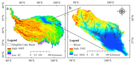
Figure 1.
Location of the Qinghai Lake Basin (b) on the Qinghai–Tibet Plateau (a).
2.2. Data Source and Processing
The spatial dataset used to simulate the distribution of future land use is listed in Table 1, including historical and current land use maps, terrain conditions (elevation and slope), socio-economic data (population density and per capita GDP), climatic and ecological factors (temperature, precipitation, and normalized difference vegetation index (NDVI)). All the spatial data were projected using the Albers equal-area conic projection (Krasovsky_1940_Albers).

Table 1.
List of data used in this study.
The simulation process in this study utilized the land use maps for the coverage area from the 1990, 2000, 2010, and 2018 calendar years. The land use classes were re-classified into the following eight categories to simplify the model: cropland, woodland, grassland, wetland, water area, developed land, desert, and glacier (Table 2). The digital elevation model (DEM) was used to extract the natural driving factors of land use transformation in the QLB, including grid information such as elevation and slope.
Table 2.
Reclassification of land use types in the QLB.
LULC changes are the result of the long-term, comprehensive effects of natural and socio-economic factors. The selection of driving factors depends on the research objectives, regional characteristics, and the availability of data. Based on the status of the study area, this study took elevation, slope, annual average temperature, and annual precipitation as the natural driving factors; population density and per capita GDP as the social driving factors; and NDVI as the ecological factor of land use transformation in the QLB (Figure 2). The spatial data were taken from several sources, including geocoding location coordinates. Spatial data manipulations, such as clipping and merging, were conducted to fit the coverage area. Then, principal component analysis (PCA) was used to reduce the redundancy between data and the subjectivity of factor selection. In the end, the cumulative method contribution rate of elevation, precipitation, GDP, slope, and population density reached 99.99%, and these were the main driving factors of LULC changes in this study. ArcGIS 10.2.2 (ESRI, Inc., Redlands, California, USA) was used to analyze and extract the natural and social driving factors of land use transformation.
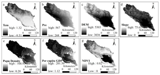
Figure 2.
Driving factors of land use change in the QLB. (a) annual average temperature; (b)annual precipitation; (c) DEM; (d) slope; (e) population density; (f) per capita GDP; and (g) NDVI.
2.3. Methodology
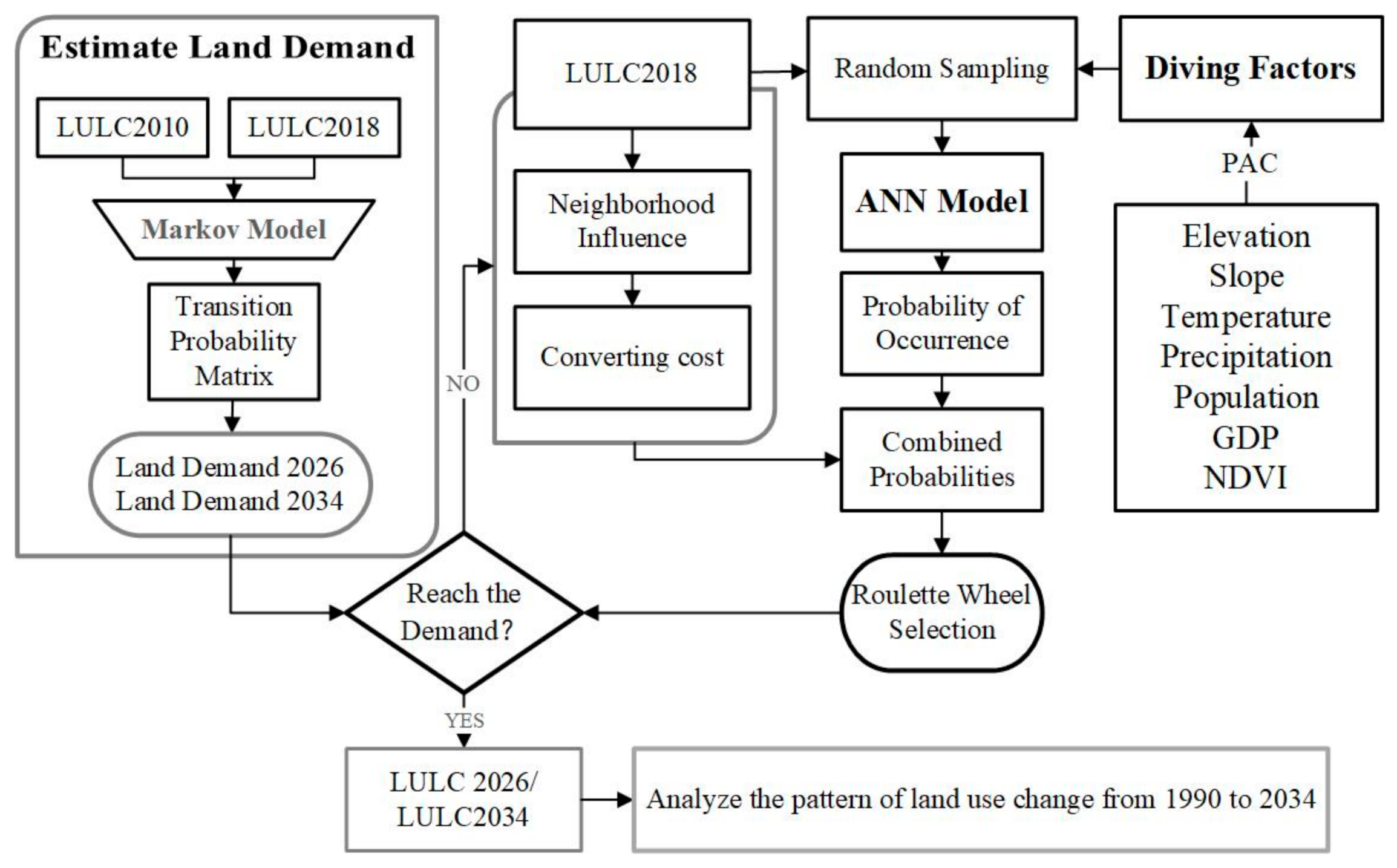
The purpose of this study was to investigate landscape pattern changes from 1990 to 2018 through the analysis of LULC maps and to forecast changes in the QLB over the next 16 years, from 2018 to 2034, using the FLUS v2.4 Model. The Markov model is a stochastic method used to describe the land demand with a transition probability matrix in land use change analysis [36] and has been widely used in ecological modeling to predict land use demand under future scenarios [37]. Based on the quantity of land use, the FLUS model was applied to simulate the spatial distribution of land use in the future. On this basis, statistical methods and a transfer matrix were used to analyze the land use pattern and identify the spatiotemporal change characteristics of land use in different periods. The future scenario assumes that development in the study area in the near future will proceed without natural disasters or sudden swings and changes in the economy and public policy. In the present study, the future scenario refers to a scenario in which the trends of changes in LULC from 2010 to 2018 will continue unaltered until 2026 and 2034, regardless of the modeling variables and human factors. The methodological framework used in the study for the simulation of the LULC is shown in Figure 3.
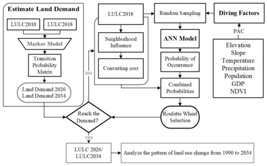
Figure 3.
Methodological framework for land use spatial distribution simulation and trend analysis.
2.4. Future Land Use Simulation Model (FLUS)
The FLUS model, proposed by Liu et al. [38], is a cellular automata (CA)–based model that has been successfully applied for the simulation of complex LULC using driving forces [38,39] and attains a higher simulation accuracy than that of other LULC simulation models, such as CLUE-S and CA [38]. This approach is an integration of two main procedures: system dynamic (SD) and CA modeling. The SD model is grounded on feedback concepts to manage non-linear, multi-loop, and time-lag characteristics of complex dynamic systems [40] and is widely used to estimate the future land use demand under various socio-environmental changes [41]. The CA model is used to allocate the future LULC through an integrated mechanism designed to process the complex interactions among the different LULC types [42]. Spatial data that have been pre-processed were used for the simulation process using the FLUS model. The simulation process with the CA approach was implemented in several stages [38] (Figure 3). The first step was estimating the probability of occurrence using the artificial neural network (ANN) model to define how driving factors affected the initial land use map. The ANN model was applied to calculate the probability of occurrence in each pixel. The next stage included the land use allocation process via the CA model.
The conversion processes of the different land use types are commonly influenced by the following: (a) the probability of occurrence; (b) the conversion cost of land use pairs, which indicates the difficulty of conversion from one LULC class to another; as such, it is a mathematical method to show the direction of land transfer. Among them, 0 represents a higher cost of land conversion, and land expansion potential is small, and 1 represents a lower cost of land conversion and greater potential for land expansion. Based on the land use transfer matrix from 2000 to 2018, combined with the land development policy of the QLB, the final cost matrix of land use change was determined (Table 3). (c) The neighborhood weights of the individual land use types in the competition mechanism based on the principles of the CA model. The neighborhood weights characterize the expansion of the different land use types; 0 represents a poorer expansion ability of land conversion and 1 represents a more notable expansion ability of land conversion. All kinds of land have different probabilities of land change in the process of land transfer, and the expansion probability varies among different land use types. In this study, the development of social economy, the improvement of infrastructure, and the rise of tourism are the main drivers of land use change. The GGP was implemented in 2000 and aimed to partially convert cropland into forest/grassland. In addition, environmental protection and restoration projects in the QLB were also implemented. Therefore, it is important to comprehensively consider the environmental characteristics and economic development of the QLB, and the analytic hierarchy process (AHP) was used to determine the neighborhood weights. The weight scores of landscape types are as follows: cropland, 0.5; woodland, 0.5; grassland, 1; wetland, 1; water area, 1; developed land, 1; desert, 1; and glacier and snow cover, 0.2. (d) The determination of land demand using the Markov chain approach was conducted to predict future land use. Based on the LULC of the QLB in 2010 and 2018, the demand for various types of land use in 2026 and 2034 were calculated using the Markov chain module (Table 4).
Table 3.
Conversion cost of land use pairs of the QLB.
Table 4.
Total land demand pixels.
The final step was the procedure of the FLUS model, which included the production of the final predicted LULC map, using the LULC demands to guide the CA model through multiple iterations. The CA model procedure stopped when the allocated area equaled the estimated demanded area for all LULC types. The results of the simulation were land use maps in a raster format. This study used the overall accuracy and Kappa coefficient as the measurement parameters to test the prediction accuracy of the FLUS model. A large Kappa coefficient indicated a high simulation accuracy between the simulated land use result and the actual land use distribution. When the Kappa coefficient was lower than 0.8, we adjusted the original factors, reforecasted the land use demand, and re-assessed the modeling parameters.
3. Results
3.1. FLUS Model Performance
In order to investigate the future LULC of the QLB, an integration of the FLUS model and Markov chain analysis was employed. Our findings showed that the implementation of the aforementioned models along with the selected socio-environmental factors was effective to simulate future LULCs. Figure 4 illustrates a raster map that is the result of the simulation and land use allocation based on driving factors and the actual land use map. Predicted and observed maps for 2018 showed a relatively similar pattern of LULC (Figure 4), suggesting that the performance of the FLUS model in allocating LULC was accurate in the QLB. The level of agreement per class, including the overall accuracy and Kappa coefficient, is presented in Table 5. The overall accuracy and Kappa coefficient reached values of 0.98 and 0.97, respectively. The Kappa coefficient of 0.97 indicates that the accuracy can satisfy the requirements of the following research and that incorporating the natural, socio-economic, and ecological factors that cause land use changes into the FLUS model is a valuable method to predict the landscape pattern of the QLB in 2018. It is also possible to predict the 2026 and 2034 landscape patterns based on the transition matrix of the image sets from 2010 to 2018.
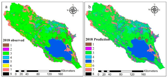
Figure 4.
Observed (a) and predicted (b) LULC maps for 2018. 1—cropland, 2—woodland, 3—grassland, 4—wetland, 5—water area, 6—developed land, 7—desert, 8—glacier.
Table 5.
Validation parameters for the results of the simulation.
3.2. LULC Changes for the Period from 1990 to 2018
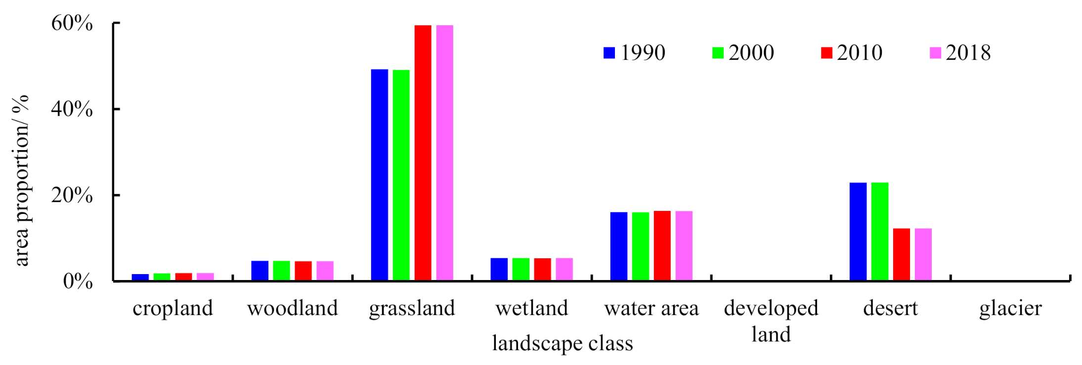
Figure 5 and Table 6 show that the grassland area increased greatly and the desert area decreased greatly, which were the most significant transformations of landscape type, while the other landscape types in the QLB showed little change. According to the dynamic change of landscape types (Figure 5), grassland was the main landscape type in the QLB, with the area proportion increasing from 49.11% in 1990 to 59.44% in 2018. The desert area decreased from 22.86% in 1990 to 12.25% in 2018. The water area was relatively stable, with an area proportion between 16.02% and 16.33%. The wetland was also relatively stable, with an area proportion between 5.37% and 5.36%. The woodland area proportion decreased from 4.74% in 1990 to 4.62% in 2018. The cropland area proportion increased from 1.66% in 1990 to 1.89% in 2018. The area proportion of grassland, cropland, and developed land continued to increase, while the proportion of water and wetland areas fluctuated upward.

Figure 5.
The proportion of landscape types in the QLB from 1990 to 2018.
Table 6.
Transition matrix of landscape types in the QLB from 1990 to 2018 (×104 m2).
According to the transition matrix of landscape types from 1990 to 2018 (Table 6), a large area of desert was transformed into grassland, and the sharp increase of grassland area was the most significant feature during this period. In general, the amount of increase of landscape areas in order from greatest to least in the study period was as follows: grassland > water area > cropland > developed land > glacier, which increased by 30.32 × 10⁸ m2, 73.54 × 10⁶ m2, 66.43 × 10⁶ m2, 8.66 × 10⁶ m2, and 9.60 × 10⁵ m2, respectively. The amount of decrease of landscape areas in order from greatest to least in the study period was as follows: desert > woodland > wetland, which decreased by 31.43 × 10⁸ m2, 35.36 × 10⁶ m2, and 2.90 × 10⁶ m2, respectively. In terms of the direction of transfer, the cropland was mainly transformed into grassland, with an area of 22.02 × 10⁶ m2; woodland was mainly transformed into grassland, with an area of 63.95 × 10⁶ m2; grassland was mainly transformed into cropland and desert, with an area of 88.69 × 10⁶ m2 and 7.40 × 10⁷ m2, respectively; wetland was mainly transformed into grassland, with an area of 43.57 × 10⁶ m2; water area was mainly converted to desert, with an area of 29.21 × 10⁶ m2; developed land was mainly converted to grassland, with an area of 8.70 × 10⁶ m2; desert was mainly transformed into grassland, with an area of 31.86 × 10⁸ m2; and glacier was mainly converted into desert, with an area of 5.70 × 10⁵ m2.
Based on the boundary of the QLB, the spatial distribution maps of the landscape types of the QLB in 1980 and 2018 (Figure 6) were obtained. From the perspective of the spatial distribution of landscape types from 1990 to 2018 (Figure 6), the desert was mainly located in the northwest of the basin, with an area proportion of 22.8%, and exhibiting a concentrated and massive distribution. After 2000, a large area of desert was transformed into grassland with the most significant change, and the area of grassland increased from 49.21% in 1990 to 54.44% in 2018. Qinghai Lake is located in the southeast of the basin, with an average area proportion of 16.16%, which was relatively stable with little change over the years. Grassland was the main landscape type in the basin and was evenly distributed in patches, with an increase in area proportion from 49.11% in 1990 to 59.44% in 2018. The wetland was mainly distributed in the middle- and high-altitude areas of the upper reaches of the Haergai River and the Shaliu River at the southern foot of the Qilian Mountains in the northern part of the basin, presenting a scattered distribution, and the area around the lake presented as a band-like distribution, with an area of 5.35% to 5.37%, which was relatively stable. The cropland was mainly distributed on the northern and southern banks of the Qinghai Lake and was lumpy, with an area proportion between 1.66% and 1.89%.
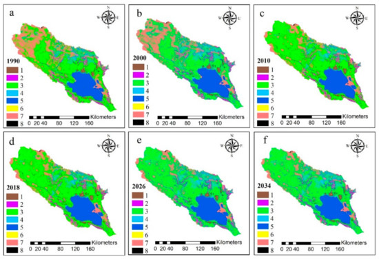
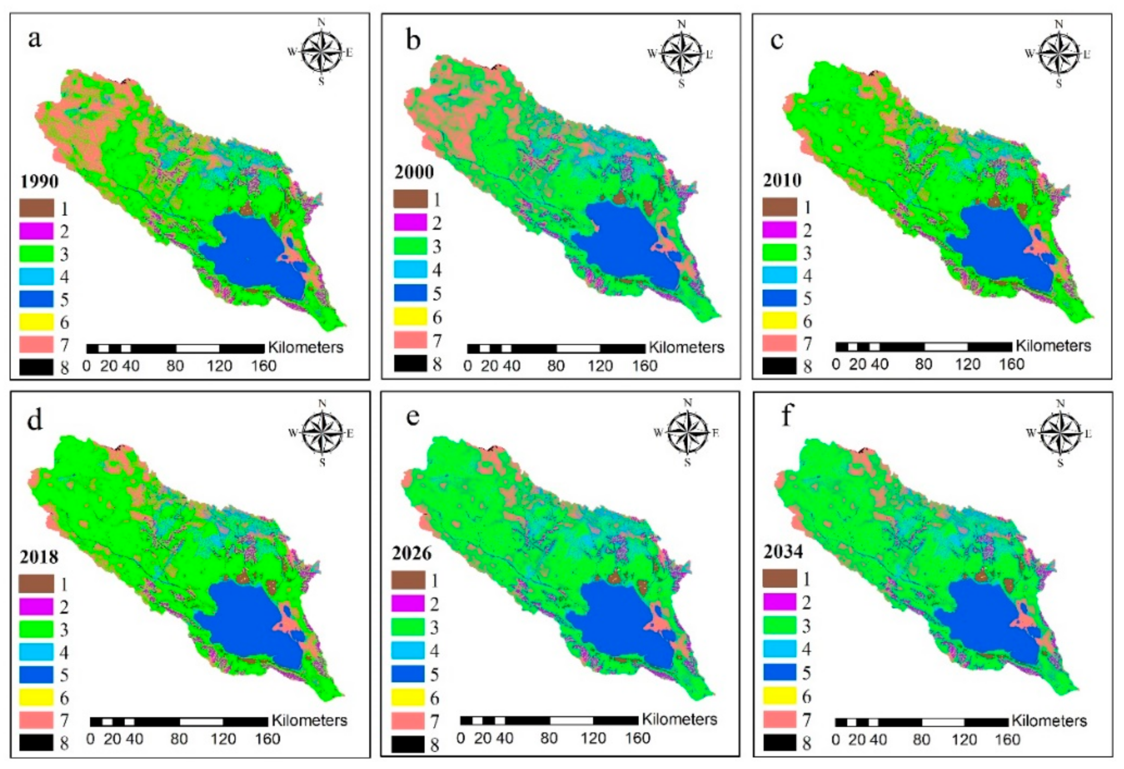
Figure 6.
Spatial distribution of landscape types in the QLB. (a) 1990, (b) 2000, (c) 2010, (d) 2010, (e) simulated 2026, and (f) simulated 2034. 1—cropland, 2—woodland, 3—grassland, 4—wetland, 5—water area, 6—developed land, 7—desert, 8—glacier.
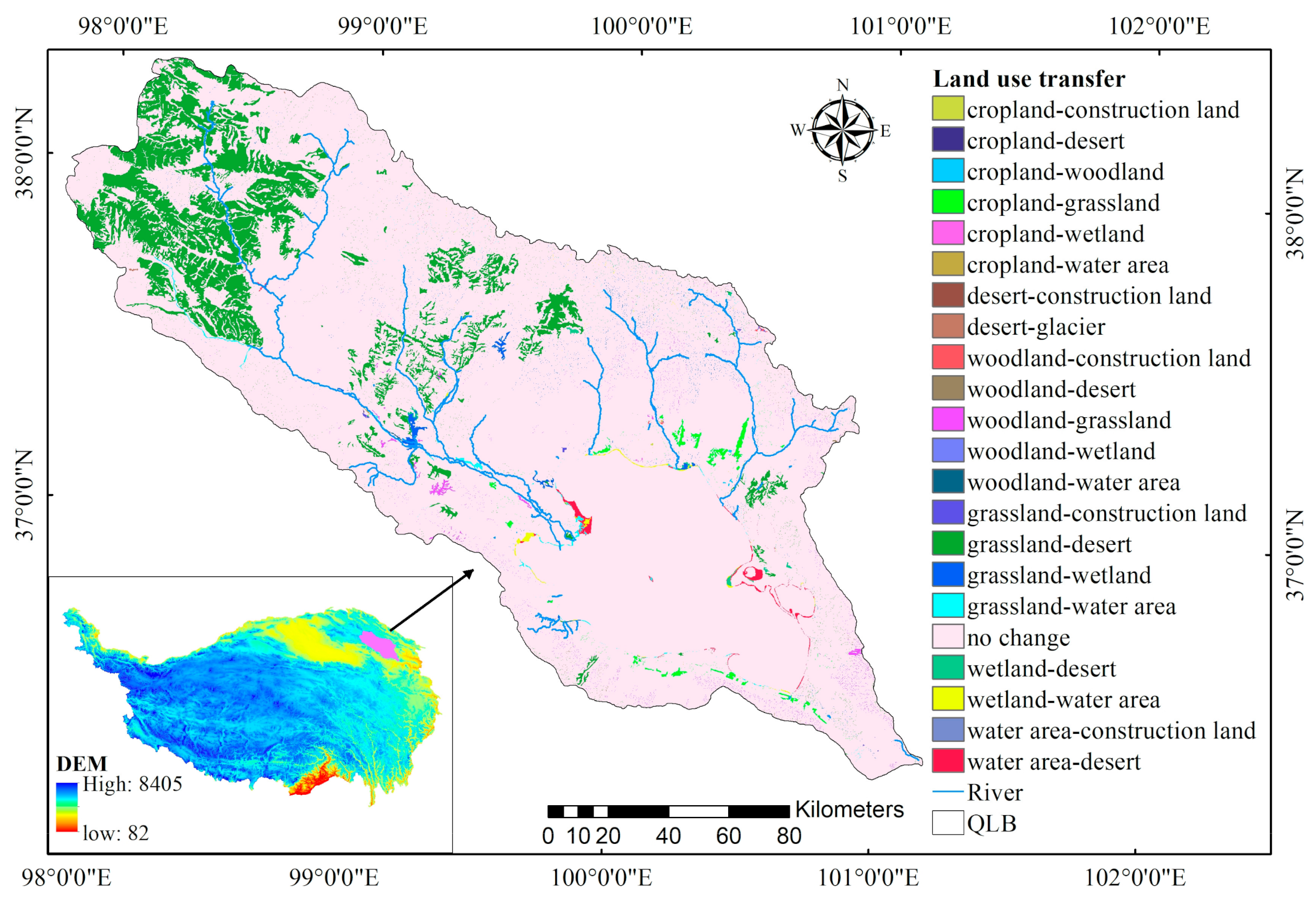
From the perspective of the direction of landscape type transfer (Figure 7), the proportion of the total area of landscape type transfer in the basin from 1990 to 2018 was 12.88%, of which the amount of transfer between grassland and desert (grassland–desert) was the largest, with an area ratio of 11.00%. The transfer between grassland and desert mainly occurred in the northwest of the basin, the northeast of Qinghai Lake, and the surrounding area in the south, presenting a concentrated and massive distribution. The area ratio between cropland and grassland transfer (cropland–grassland) was 0.37%, which was mainly distributed in the northern and southern banks of Qinghai Lake and southeast of the surrounding area of Qinghai Lake, presenting a banded distribution. The area ratio between woodland and grassland transfer (woodland–grassland) was 0.33%, which mainly occurred in the Buha River, the entrance of the Buha River, and the northeastern part of the basin, showing a patchy distribution. The area ratio between grassland and wetland transfer (grassland–wetland) was 0.32%, which was mainly distributed along the banks of the Buha River and the lakeshore around Qinghai Lake and presented a zonal distribution. The area ratio between water area and desert transfer (water area–desert) was 0.28% and was mainly distributed in the lake entrance of the Buha River, the East Lake Sha Island, and the vast transitional zone of water and land around the lake, presenting a concentrated block distribution and fine strip distribution. The area ratio between the grassland and water area transfer (grassland–water area) was 0.23%, which was mainly distributed along the main stream of the Buha River and at the entrance to the lake, presenting a banded and scattered distribution.

Figure 7.
Spatial distribution of land use transfer flows in the QLB from 1990 to 2018.
3.3. Estimated LULC Changes for the Period from 2018 to 2034
Based on the changes of landscape types from 2010 to 2018, the FLUS model was used to predict the quantitative changes and spatial distribution of landscape patterns in 2026 and 2034 under natural scenarios. From the perspective of the number of landscape patterns (Table 7), all the landscape types were generally stable with little change. The proportions of cropland, woodland, and desert of 1.89%, 4.61%, and 59.46%, respectively, were relatively stable. Wetlands showed a continuous and gradual increasing trend from 5.36% in 2018 to 5.44% in 2034. Developed land showed a gradual increasing trend from 0.10% in 2018 to 0.12% in 2034. The water area showed a continuous and slow decrease from 16.28% in 2018 to 16.16% in 2034. In terms of spatial distribution (Figure 6), the spatial distribution pattern of the QLB landscape pattern in 2026 and 2034 was similar to that in 2018, with little change.
Table 7.
LULC area values for the period 2018–2034 in the QLB (m2).
According to the transfer matrix of landscape types from 2018 to 2034 (Table 8), the quantity of each landscape type was basically stable with little change. A decrease in the water area and an increase in the area of wetlands were the main characteristics of this period. In general, the amount of increase in landscape areas in order from greatest to least in the study period was as follows: wetland > grassland > developed land > cropland > glacier, which increased by 23.86 × 10⁶ m2, 7.14 × 10⁶ m2, 4.71 × 10⁶ m2, 1.27 × 10⁶ m2, and 8.10 × 10⁵ m2, respectively. The amount of decrease in landscape areas in order from greatest to least in the study period was as follows: water area > woodland > desert decreased by 33.22 × 10⁶ m2, 4.29 × 10⁶ m2, and 2.80 × 10⁵ m2, respectively. In regard to the direction of transfer, cropland was mainly transformed into grassland, with an area of 12.80 × 10⁶ m2; woodland was mainly transformed into grassland, with an area of 75.73 × 10⁶ m2; grassland was mainly transformed into woodland and desert, with an area of 73.63 × 10⁶ m2 and 92.05 × 10⁶ m2, respectively; wetlands were mainly transformed into grassland, with an area of 53.53 × 10⁶ m2; water areas were mainly converted to desert and grassland, with an area of 28.33 × 10⁶ m2 and 24.33 × 10⁶ m2, respectively; and desert was mainly transformed into grassland with an area of 93.41 × 10⁶ m2.
Table 8.
Transition matrix of landscape types in the QLB from 2018 to 2034 (×104 m2).
4. Discussion
With the progress of society and economic development, the QLB has developed rapidly due to the unique plateau scenery and ethnic culture, as well as the changes taking place in LULC. These changes should be monitored and analyzed in order to adjust relevant policies. Our study revealed the positive impact of the implementation of national environmental protection policies on the change of the local landscape types.
In this study, the land use maps of 1990, 2000, 2010, and 2018 were integrated with a combination of the CA-Markov model and the FLUS model, the LULC predictions for the QLB in 2026 and 2034 were presented for a total of eight classes under natural scenarios. The overall accuracy and Kappa coefficient reached values of 98.47% and 0.97, respectively, by overlaying the 2018 simulation map and the 2018 land use map showing the model’s performance. A Kappa coefficient > 0.8 indicated that the accuracy of the simulation model was statistically credible [43] and that the FLUS model had good applicability in the study area. User’s and producer’s accuracy for all classes ranged from 71% to 99%, with developed lands and grasslands showing the lowest and the highest level of agreement, respectively. Therefore, using the FLUS and Markov models and considering the natural factors (annual mean temperature, annual precipitation, elevation, and slope), socio-economic factors (population density, per capita GDP), and ecological factors (NDVI) is a reliable method to predict the future spatial changes of landscape types in the QLB. The accuracy result was in line with that of other studies [28] that aimed to simulate multiple LULCs in the QLB using CA-based models.
During the 28-year period from 1990 to 2018, the grassland area of the QLB increased by 30.32 × 10⁸ m2, and the desert decreased by 31.43 × 10⁸ m2. From the land use transfer matrix, an area of 31.86 × 10⁸ m2 of the desert was transformed into the grassland, accounting for 10.75% of the total area of the basin. From the perspective of the direction of landscape type transfer, the desert–grassland transfers were mainly distributed in the northwestern part of the basin, the northeastern Qinghai Lake, and the southern lake area, accounting for 11% of the total area of the basin. The occurrence of this phenomenon was mainly the result of the combined effect of natural and human factors, with the human factors dominating. In terms of natural factors, during the study period, the temperature in the QLB increased [44], precipitation increased [45], the climate tended to be warm and humid [45,46], and the lake area expanded [46,47]. A large area of desert in the middle- and high-altitude areas of the northwestern in the QLB was transformed into low-coverage grassland, and the coverage of vegetation greatly increased [26]. An increase in water volume has improved vegetation cover and groundwater runoff, causing the basin to form a benign hydrological cycle [48] as well as leading to significant improvement in the total ecological environment [49]. In terms of human factors, since the Party Central Committee and the State Council implemented the major decisions and deployments of the Western Development Strategy in 2000, Qinghai Province has initiated a large number of ecological construction projects to protect and improve the environment. In particular, the implementation of the GGP for seven consecutive years since 2000 has effectively promoted the improvement of the ecological environment of the river source areas [50]. In addition, a 10-year (2007–2017) Japanese Yen loan project called the “QLB Ecological Environment Comprehensive Management Project” with a total investment of CNY 540 million was initiated in 2006 [51]. The project has effectively restored and protected the vegetation in the QLB, maintained the stability of the grassland and forest ecosystems, and achieved the restoration of ecological functions and the goal of good ecology through the treatment of degraded grassland, wind-proofing and sand-fixing, afforestation, and water and soil conservation. Furthermore, the Qinghai Lake Scenic Area Protection and Utilization Administration Bureau, established in 2007, held a press conference in March 2020 and publicly released the “Qinghai Lake Ecological Environment Protection Status”, aiming to inform and educate the public on the ecological status of Qinghai Lake, the ecological protection process, the protection management measures, and the effectiveness of ecological protection [52].
The Markov model and the FLUS model were used to comprehensively consider the impact of natural, socio-economic, and ecological factors on landscape type changes based on the transition direction of landscape types from 2010 to 2018 and to simulate the distribution of land use in 2026 and 2034 under natural conditions. In the simulation of the 16-year period from 2018 to 2034, the proportion of the number of various landscape types changed little, the spatial distribution was stable, and the changes between different landscape types were minor. The area proportions of cropland, woodland, desert, and grassland changed slightly at 1.89%, 4.61%, 12.26%, and 59.46%, respectively. Grassland and desert were the main landscape types in the basin, accounting for 71.72% of the total area of the basin. The main landscape area showed little change and the spatial matching was stable, indicating that the ecological environment of the study area will be in a balanced and stable state over the next 16 years. The developed land has been increasing slowly, from 0.10% in 2018 to 0.12% in 2034. In 2019, the total population of the QLB was 23.72 × 10⁴. The permanent population is small, and the seasonal changes in the tourist population were significant. In order to promote the development of tourism, infrastructure will need continuous improvement, and developed land area will continue to increase. In the simulation, the area of water areas decreased from 16.28% in 2018 to 16.16% in 2034, showing a continuous and gradual decrease. This result is essentially consistent with that of using comprehensive statistical methods and the regional climate model system, Providing Regional Climates for Impacts Studies (PRECIS) [53]. The simulation results of future landscape types showed that the area of the main landscape types of woodlands, grasslands, and deserts in the QLB over the next 16 years (2018–2034) will change little, and the spatial structure will be stable. The area of farmlands and developed lands for man-made landscapes will increase, and water bodies will slowly decrease. As an important international wetland and biodiversity conservation area, the QLB has a fragile ecological environment. It is very important to weigh the relationship between nature protection and economic development in future land management. An increase in croplands and developed lands will inevitably affect the ecological security pattern of the lake area. The government should uphold the principle of prioritizing ecological protection, limit human disturbance in key ecological areas, continue to implement the ecological protection projects such as the GGP, maintain grassland ecological compensation, and reduce the intensity of grazing in grasslands around the lake. In view of shrinking bodies of water, the protection of aquatic organisms and the biodiversity of their habitats will become a focus of attention.
While leaving the existing environmental variables and policies unchanged, the FLUS model was used to predict the number and spatial distribution of landscape types in the Qinghai Lake Basin in 2026 and 2034. The short-term forecast results were credible, and the long-term forecast results may be biased [54]. The reason for the deviation lies in the inability to make timely adjustments and changes to the simulation results according to policies and systems. This study simulated future land use changes based on the trends in environmental variables and national policies that have had an impact. The policy is contingent and phased. The continued implementation of the protection policy makes the long-term forecast results of this study basically consistent with the future situation; however, the implementation of the resource development policy may make the forecast results differ from the future situation. Therefore, it is possible to compare the land use change trends in multiple scenarios in the following study and reveal the possible development trends of key areas under different scenarios that can be used to put forward corresponding land management suggestions for different development goals.
5. Conclusions
This study presented the long-term (1990 to 2034) spatial–temporal characteristics of landscape patterns of the QLB using the Markov and FLUS models. The main conclusions of this study can be summarized as follows:
- (1)
- A comprehensive consideration of the natural, economic, and ecological factors, using the Markov model and the FLUS model, based on the change direction of landscape types from 2010 to 2018, can be used to predict the numerical changes and spatial distribution characteristics of landscape types in 2026 and 2034. At the same time, the simulated 2018 landscape type map and the 2018 actual landscape type map were used to evaluate the accuracy of the model. The results show that the overall accuracy and Kappa coefficient distribution of the FLUS model were 0.98 and 0.97, indicating the simulation results were relatively reliable.
- (2)
- During the period from 2000 to 2018, the grassland area of the QLB increased by 30.32 × 10⁸ m2, the desert area decreased by 31.43 × 10⁸ m2, and 31.86 × 10⁸ m2 of desert was transformed into grasslands, accounting for 10.75% of the total area of the basin, indicating that the desert areas have been greatly reduced and converted into grasslands. The direct reason for the significant expansion of the grassland area is the implementation of policies and activities, such as the project of the GGP, the comprehensive management of the ecological environment in the QLB, and the ecological environment protection of the QLB. At the same time, the transformation of deserts into grasslands also benefited from natural factors, such as the climate in the basin tending to be warm and wet, resulting in an increase in vegetation coverage, and an active water cycle during this period.
- (3)
- In the 16-year period from 2018 to 2034, the proportion of various landscapes will change slightly, and meanwhile the spatial distribution will be stable.
Author Contributions
Conceptualization, K.C. and D.Y.; methodology, Y.H.; software, Y.H.; validation, Y.H.; formal analysis, Y.H.; investigation, Y.H.; resources, Y.H.; data curation, Y.H.; writing—original draft preparation, Y.H.; writing—review and editing, Y.H. and D.Y.; visualization, Y.H.; supervision, K.C. and D.Y.; project administration, K.C. and D.Y.; funding acquisition, K.C. All authors have read and agreed to the published version of the manuscript.
Funding
The research work was supported by the National Natural Science Foundation of China (grant no. 41661023, grant no. 41971269), the Second Tibetan Plateau Scientific Expedition Program (grant no. SQ09QZkk0405).
Data Availability Statement
The data presented in this study are openly available in Institute of Geographic and Natural Resources Research, Chinese Academy of Sciences (CAS) (https://www.resdc.cn/, (accessed on 25 May 2020)), Resource and Environment Data Cloud Platform (https://www.gscloud.cn/, (accessed on 25 May 2020)), and Level-1 and Atmosphere Archive and Distribution System Distributed Active Archive Center (LAADS DAAC) (https://ladsweb.modaps.eosdis.nasa.gov/, (accessed on 25 May 2020)), see Table 1 for details.
Acknowledgments
We gratefully acknowledge financial support from the Key Laboratory of Qinghai Province Physical Geography and Environmental Process, MOK Key Laboratory of Tibetan Plateau Land Surface Processes and Ecological Conservation. We also want to express our respect and thanks to the anonymous reviewers and the editors for their important and insightful comments and suggestions, which helped improve the manuscript.
Conflicts of Interest
The authors declare no conflict of interest.
References
- Salazar, A.; Baldi, G.; Hirota, M.; Syktus, J.; Mcalpine, C. Land use and land cover change impacts on the regional climate of non-Amazonian South America: A review. Glob. Planet. Chang. 2015, 128, 103–119. [Google Scholar] [CrossRef]
- Gutman, G.; Justice, C.; Sheffner, E.; Loveland, T. The NASA Land Cover and Land Use Change Program; Land Change Science; Springer: Berlin/Heidelberg, Germany, 2012; pp. 17–29. [Google Scholar]
- Gao, F.; Ma, Q.; Shan, P.; Yang, D.; Guo, X.; Yang, S.; Zhang, Z. Land Use/Cover Change and Hot Spots Analysis in Muffling City of Heilongjiang Province. Areal Res. Dev. 2016, 35, 126–130. [Google Scholar]
- Jaarsveld, A.; Biggs, R.; Scholes, R.J.; Bohensky, E.; Fabricius, C. Measuring conditions and trends in ecosystem services at multiple scales: The Southern African Millennium Ecosystem Assessment (SAfMA) experience. Philos. Trans. R. Soc. Lond. 2005, 360, 425–441. [Google Scholar] [CrossRef] [Green Version]
- Liu, J.; Kuang, W.; Zhuang, Z.; Xu, X.; Qin, Y.; Ning, J.; Zhou, W.; Zhang, S.; Li, R.; Yan, C.; et al. Spatiotemporal characteristics, patterns and causes of land use changes in China since the late 1980s. J. Geogr. Sci. 2014, 24, 195–210. [Google Scholar] [CrossRef]
- Mooney, H.A.; Duraiappah, A.; Larigauderie, A. Evolution of natural and social science interactions in global change research programs. Proc. Natl. Acad. Sci. USA 2013, 110, 3665–3672. [Google Scholar] [CrossRef] [Green Version]
- Wang, C.; Zhang, B.; Zhang, S. Study on the effects of land use change on ecosystem service values of Jilin Province. J. Nat. Resour. 2004, 19, 55–61. [Google Scholar]
- Ramachandra, T.V.; Bharath, S.; Gupta, N. Modelling landscape dynamics with LST in protected areas of Western Ghats, Karnataka. J. Environ. Manag. 2018, 206, 1253–1262. [Google Scholar] [CrossRef] [PubMed]
- Aksoy, H.; Kaptan, S. Simulation of Future Forest and Land Use/Cover Changes (2019–2039) Using the Cellular Automata-Markov Model. Geocarto Int. 2020, 1–17. [Google Scholar] [CrossRef]
- Sterling, S.M.; Ducharne, A.; Polcher, J. The impact of global land-cover change on the terrestrial water cycle. Nat. Clim. Chang. 2013, 3, 385–390. [Google Scholar] [CrossRef]
- Ridding, L.E.; Newton, A.C.; Redhead, J.W.; Watson, S.; Rowland, C.S.; Bullock, J.M. Modelling historical landscape changes. Landsc. Ecol. 2020, 35, 2695–2712. [Google Scholar] [CrossRef]
- Bartuszevige, A.M.; Kennedy, P.L.; Taylor, R.V. Sixty-Seven Years of Landscape Change in the Last, Large Remnant of the Pacific Northwest Bunchgrass Prairie. Nat. Areas J. 2014, 32, 166–170. [Google Scholar] [CrossRef]
- Deng, Q.; Ou, Z.; Deng, Z.; Zhen, M.; Sun, S.; Li, C.; Ma, Y. Changes of Landscape Pattern and Driving Factors in Menghai. J. Southwest For. Univ. 2019, 39, 118–126. [Google Scholar]
- Cao, Q.; Chen, X.; Shi, M.; Yao, Y. Land use/cover changes and main-factor driving force in Heihe middle reaches. Trans. Chin. Soc. Agric. Eng. 2014, 30, 220–227. [Google Scholar]
- Zhang, M.; Gong, Z.; Zhao, W.; A, D. Landscape pattern change and the driving forces in Baiyangdian wetland from 1984 to 2014. Acta Ecol. Sin. 2016, 36, 4780–4791. [Google Scholar]
- Yang, R. Spatiotemporal change and driving forces of urban landscape pattern in Beijing. Acta Ecol. Sin. 2015, 35, 4357–4366. [Google Scholar]
- Ren, J.; Liu, H.; Ding, S.; Wang, M.; Qi, Z. Landscape pattern change and its driving mechanism in Yihe River basin, China. Chin. J. Appl. Ecol. 2017, 28, 2611–2620. [Google Scholar]
- Fu, B.; Pan, N. Integrated studies of physical geography in China: Review and prospects. J. Geogr. Sci. 2016, 26, 771–790. [Google Scholar] [CrossRef] [Green Version]
- Cao, R.; Qi, W.; Li, L.; Jiang, W.; Cao, X. Catchment-based landscape patterns and divisions in mountain areas: A case study of Qixia City in Shandong Province. Chin. J. Eco-Agric. 2014, 22, 859–865. [Google Scholar]
- Luo, C.; Xu, C.; Cao, Y.; Tong, L. Monitoring of water surface area in Lake Qinghai from 1974 to 2016. J. Lake Sci. 2017, 29, 1245–1253. [Google Scholar]
- Tian, Y.; Wu, F.; Zhang, L.; Li, F.; Cao, J. Ecological Environment Characteristics of the Soil around Qinghai Lake under the Influence of Human Activities. Saf. Environ. Eng. 2013, 20, 77–81. [Google Scholar]
- Zhou, D.; Ma, H.; Shan, F.; Huang, H.; Wu, F.; Cao, G.; Chen, Z.; Gao, D. Pasture Resources and Ecological Protection in Qinghai Lake Drainage Basin and Surrounding Areas. Resour. Sci. 2006, 28, 94–101. [Google Scholar]
- Qinghai Lake Is Always the Most Beautiful Lake. Available online: http://www.qhnews.com/qhly/system/2008/05/27/002519376.shtml (accessed on 19 June 2021).
- Wang, H.; Wang, F.; Zhang, X.; Yan, H. Eco-environmental Evolution and Stability of Qinghai Lake. Yellow River 2011, 33, 35–38. [Google Scholar]
- Han, Y.; Chen, K.; Yu, D. Evaluation on the Impact of Land Use Change on Habitat Quality in Qinghai Lake Basin. Ecol. Environ. Sci. 2019, 28, 2035–2044. [Google Scholar]
- Bao, W.; Zhang, Y.; Dai, L.; Zhao, G.; Jiang, K. Spatio-temporal Change Analysis of Vegetation Coverage Based on the Liner Spectral Mixture Model in Qinghai Lake Basin. Hubei Agric. Sci. 2018, 57, 44–48. [Google Scholar]
- Chen, K.; Li, S.; Zhou, Q.; Duo, H.; Chen, Q. Analyzing Dynamics of Ecosystem Service Values based on Variations of Landscape Patterns in Qinghai Lake Area in Recent 25 Years. Resour. Sci. 2008, 30, 274–280. [Google Scholar]
- Lei, H.; Wang, L. Simulation of Land Use Change in Qinghai Lake Watershed Based on CA-Markov Model. J. Anhui Agric. Sci. 2015, 43, 328–331, 336. [Google Scholar]
- Ma, H.; Guo, L.; Ma, Y.; Xie, Y. Landscape Characteristics of Northern Shore of Qinghai Lake and Analysis on Landscape Pattern Based on TM Data. J. Anhui Agric. Sci. 2010, 38, 6865–6866+7040. [Google Scholar]
- Zhang, F.; Chen, K.; Duo, H.; Su, M. Study on Changes of Grassland Landscape Pattern in Qinghai Lake Watershed. J. Landsc. Res. 2009, 1, 39–43. [Google Scholar]
- Pepin, N.; Bradley, R.S.; Diaz, H.F.; Baraer, M.; Caceres, E.B.; Forsythe, N.; Fowler, H.; Greenwood, G.; Hashmi, M.Z.; Liu, X.D. Elevation-dependent warming in mountain regions of the world. Nat. Clim. Chang. 2015, 5, 424–430. [Google Scholar]
- Lu, R.; Jia, F.; Gao, S.; Shang, Y.; Li, J.; Zhao, C. Holocene aeolian activity and climatic change in Qinghai Lake basin, northeastern Qinghai–Tibetan Plateau. Palaeogeogr. Palaeoclimatol. Palaeoecol. 2015, 430, 1–10. [Google Scholar] [CrossRef]
- Guo, W.; Xiang, N.; Jing, D.; Shang, Y.; Li, J.; Zhao, C. Spatial-temporal patterns of vegetation dynamics and their relationships to climate variations in Qinghai Lake Basin using MODIS time-series data. J. Geogr. Sci. 2014, 24, 1009–1021. [Google Scholar] [CrossRef]
- An, Z.; Colman, S.M.; Zhou, W.; Li, X.; Brown, E.T.; Jull, A.T.; Cai, Y.; Huang, Y.; Lu, X.; Chang, H. Interplay between the Westerlies and Asian monsoon recorded in Lake Qinghai sediments since 32 ka. Sci. Rep. 2012, 2, 619. [Google Scholar] [CrossRef] [PubMed]
- Sun, Y.J.; Lai, Z.P.; Madsen, D.; Hou, G.L. Luminescence dating of a hearth from the archaeological site of Jiangxigou in the Qinghai Lake area of the northeastern Qinghai-Tibetan Plateau. Quat. Geochronol. 2012, 12, 107–110. [Google Scholar] [CrossRef]
- Moghadam, H.S.; Helbich, M. Spatiotemporal urbanization processes in the megacity of Mumbai, India: A Markov chains-cellular automata urban growth model. Appl. Geogr. 2013, 40, 140–149. [Google Scholar] [CrossRef]
- Pijanowski, B.; Duh, J.D.; Brown, D.G. Modeling the Relationship between land use and land cover on private lands in the Upper Midwest, USA. J. Environ. Manag. 2000, 59, 247–263. [Google Scholar]
- Liu, X.; Liang, X.; Li, X.; Xu, X.; Ou, J.; Chen, Y.; Li, S.; Wang, S.; Pei, F. A future land use simulation model (FLUS) for simulating multiple land use scenarios by coupling human and natural effects. Landsc. Urban Plan. 2017, 168, 94–116. [Google Scholar] [CrossRef]
- Liang, X.; Liu, X.; Chen, X.; Tian, Y.; Yao, H. Delineating multi-scenario urban growth boundaries with a CA-based FLUS model and morphological method. Landsc. Urban Plan. 2018, 177, 47–63. [Google Scholar] [CrossRef]
- Bottero, M.; Datola, G.; Angelis, E.D. A System Dynamics Model and Analytic Network Process: An Integrated Approach to Investigate Urban Resilience. Land. 2020, 9, 242. [Google Scholar] [CrossRef]
- Yao, H.; Shen, L.; Tan, Y.; Hao, J. Simulating the impacts of policy scenarios on the sustainability performance of infrastructure projects. Autom. Constr. 2011, 20, 1060–1069. [Google Scholar] [CrossRef]
- Kefalas, G.; Poirazidis, K.; Xofis, P.; Stamatis, K.; Chalkias, C. Landscape dynamics on insular environments of south-east Mediterranean Europe. Geocarto Int. 2020. [Google Scholar] [CrossRef]
- Chen, K.; Qi, M.; Wang, X.; Huang, G. Study of urban lake landscape ecological security pattern evolution in Wuhan, 1995–2015. Acta Ecol. Sin. 2019, 39, 245–254. [Google Scholar]
- Yin, W.; Li, X.; Cui, B.; Ma, Y. Climate Change and Impact on Water Level of the Qinghai Lake Watershed. Arid Meteorol. 2010, 28, 375–383. [Google Scholar]
- Su, F.; Zhang, C.; Hu, D. Climate change and its effect on drought in Qinghai Lake Basin. Qinghai Sci. Technol. 2018, 25, 68–74. [Google Scholar]
- Li, X.; Li, L.; Wang, G.; He, Z.; Xiao, J. Water Level and Agriculture and Husbandry Characteristics in Qinghai Lake Basin: The Response to Climate Warming and Wetting. Chin. Agric. Sci. Bull. 2017, 34, 119–127. [Google Scholar]
- Wang, H.; Liu, J.; Xie, Z.; Ma, L. Trend and Attribution Analysis of Runoff in Qinghai Lake Basin. Water Resour. Power 2018, 36, 18–21. [Google Scholar]
- Jin, Z.; Zhang, F.; Wang, H.; Bai, A.; Qin, X. The reasons of rising water level in Lake Qinghai since 2005. J. Earth Environ. 2013, 4, 1355–1362. [Google Scholar]
- Wang, Z.; Xie, J.; Liu, X.; Li, Q.; Li, X. Study on the Relationship between Vegetation Coverage and Water Area in the Qinghai Lake Basin. Environ. Sci. Surv. 2019, 38, 12–16. [Google Scholar]
- Qinghai Province Implements Conversion of Farmland to Forests/Grasslands and More than 8 Million Acres of Barren Hills Are Covered with Greenery. Available online: http://www.gov.cn/jrzg/2007-04/12/content_580375.htm (accessed on 20 June 2021).
- Foreign-Funded Projects: A Trickle to Run the Plateau. Available online: http://www.qh.gov.cn/zwgk/system/2020/08/05/010364051.shtml (accessed on 20 June 2021).
- Qinghai Lake Ecological Environment Protection Status Released. Available online: http://sthjt.qinghai.gov.cn/xwzx/szyw/202003/t20200309_84581.html (accessed on 20 June 2021).
- Li, L.; Shi, X.; Shen, H.; Dai, S.; Xiao, J. Cause of Water Level Fluctuation in Qinghai Lake from 1960 to 2009 and Its Future Trend Forecasting. J. Nat. Resour. 2011, 26, 1566–1574. [Google Scholar]
- Sun, Y.; Li, D.; Jiang, H.; Jiang, H.; Zhou, Y. Prediction of Land Use Change Based on Markov and GM(1,1)Models. J. Agric. Resour. Environ. 2016, 33, 289–296. [Google Scholar]


Publisher’s Note: MDPI stays neutral with regard to jurisdictional claims in published maps and institutional affiliations. |
© 2021 by the authors. Licensee MDPI, Basel, Switzerland. This article is an open access article distributed under the terms and conditions of the Creative Commons Attribution (CC BY) license (https://creativecommons.org/licenses/by/4.0/).